How Does Density Impact Carbon Emission Intensity: Insights from the Block Scale and an Optimal Parameters-Based Geographical Detector

Abstract

Density is a crucial indicator for urban sustainable development and is considered a critical factor influencing the carbon emission intensity of construction land (CICL). The impact of density on carbon emissions has been extensively explored, mainly focusing on grid-scale and single-factor effects. However, how density and its interactions affect carbon emissions at the block scale is unclear. Therefore, based on multiple data sources such as energy consumption, remote sensing, and the point of interest (POI) in the urban block of Changxing County, this study constructed a density system that reflects the block’s physical environment and socioeconomic characteristics. An optimal-parameters-based geographical detector was employed to investigate the effects and interactions of density factors on the carbon emission intensity of residential blocks (CIRB), carbon emission intensity of commercial blocks (CICB), and carbon emission intensity of public blocks (CIPB). The results indicate the following: (1) The impact of density factors on different types of CICL varied significantly. Physical environmental factors (PEFs) had greater explanatory power than socioeconomic factors (SEFs) across the CIRB, CICB, and CIPB, with the floor area ratio (FAR) being the most influential. The spatial morphology of blocks also influenced the relationship between density factors and the CICL. (2) The interactions between the FAR and building density (BD), the FAR and commercial outlet density (COD), and the FAR and population density (PD) had the strongest explanatory power for the CIRB, CICB, and CIPB, respectively, and all exhibited nonlinear enhancements. Some factors exhibited more significant effects only when interacting with others. (3) An association chain encompassing the interactions of multiple density factors was extracted for the CIRB, CICB, and CIPB, respectively, as the basis for conducting collaborative management and control in spatial planning. The research findings can provide decision support for urban planners to consider the comprehensive effects of density factors and promote the development of low-carbon urban spaces.

1. Introduction

Urban areas are major sources of carbon emissions [1,2]. Urban construction land, serving as the primary carrier for human economic production and daily life, is where carbon emissions are concentrated [3]. Reducing the carbon emission intensity of construction land (CICL) is crucial for addressing global climate change and achieving low-carbon urban development. By the end of 2022, China’s urbanization rate had reached 65.2% (National Bureau of Statistics data, https://www.gov.cn/xinwen/2023-02/28/content_5743623.htm, accessed on 8 November 2023). The development approach of urban areas is shifting from extensive expansion based on scale growth to refined regulation based on optimizing existing resources and enhancing intrinsic qualities [4,5]. This shift also signifies a transition in the low-carbon governance of urban spaces from promoting low-carbon construction to achieving low-carbon and efficient operation [6]. Density is an essential indicator for quantitatively describing urban spatial forms, measuring the efficiency of material resource allocation in cities, and understanding the operating principles of urban spaces [7,8]. It represents the objective distribution of various urban components per unit of land area and encompasses multidimensional attributes related to the physical environment, socio-economics, and more [9]. Density has become an essential tool in spatial planning to achieve the low-carbon and efficient operation of urban spaces by optimizing the distribution of resources. Therefore, exploring the relationship between density and the CICL will enhance the rationality and effectiveness of carbon emission control in spatial planning, thereby supporting the achievement of carbon peaking and carbon neutrality goals in cities.

Currently, exploring the impact of density on carbon emissions is a hot topic in domestic and international research. Extensive research has been carried out at regional, city, and block scales to provide a basis for achieving urban carbon emission reductions by controlling and guiding density development. The first thing that needs to be illustrated is that the existing research primarily focuses on reflecting the spatial physical characteristics of density, often represented by indicators such as the floor area ratio (FAR), building density (BD), building height (BH), or green area ratio (GAR) [10,11]. Some studies define density as population density (PD) [12,13], while exploring a density system that reflects spatial multidimensional composite attributes is still in progress. As a result, current studies exploring the relationship between density and carbon emissions are mainly conducted in the context of urban morphology, the built environment, or urban spatial structures. Density is often one of the core indicators used to investigate its relationship with energy consumption or carbon emissions related to urban land use or transportation [14,15]. Researchers have extensively investigated the relationship between typical density indicators such as the FAR, BD, BH, PD, and carbon emissions in construction land. They have utilized various methods, including correlation analysis [14,16], regression models [17,18,19], panel econometric models [20,21], and STIRPAT [22,23], to assess the impacts of these indicators on carbon emissions quantitatively.

Regarding specific research contents, the current research mainstream is to explore the relationship between carbon emissions and density based on grid-based land units at different scales. R. Gudipudi et al. investigated the relationship between PD in residential areas and carbon efficiency based on 1 km² grid units in the United States. They found that doubling the PD would typically lead to a reduction of at least 42% in carbon emissions from the building and transportation sectors [24]. It also needs to be realized that increased population density will also increase congestion in cities, affecting residents’ well-being and daily lives. F. Chen et al. explored the impact of urban density on spatial carbon performance in Shanghai based on 1 km² grid units. They discovered an inverted “U”-shaped relationship between spatial carbon performance and BD [25]. E. Resch et al. estimated the urban operational energy consumption on 1 km² grid units and explored its relationship with PD and BH. They discovered that an optimal BH exists within the range of 7–27 floors, depending on the variations in population and building lifespan [26]. S.J. Quan et al. constructed grid blocks of 200 feet by 200 feet. They simulated buildings’ annual heating and cooling energy consumption within these blocks and investigated their relationship with density. Their study revealed that under different BDs, a U-shaped relationship exists between BH and energy consumption per unit area [27]. Additionally, several studies on block-level land units explore the relationship between carbon emissions and density. For example, W.Q. Wang et al. estimated the carbon emissions of 54 communities in Shanghai’s Chaoyang Xincun through a questionnaire survey, investigating the relationship between residential density and carbon emissions. They found that the FAR, average building height (ABH), and PD exhibited segmental fluctuations with carbon emissions [28]. Q.H. Dong et al. evenly distributed grid-based carbon data onto block-level land units to investigate the relationship between urban form and carbon emissions. They found that density had bidirectional effects on carbon emissions, with a predominant positive driving effect [15].

Although current research has made significant contributions to understanding the relationship between typical density indicators and carbon emissions, there are still certain limitations. Firstly, regarding research methods, existing studies have mainly explored the impact of individual density factors on carbon emissions, overlooking the interactions among the driving factors of land carbon emissions [29]. Generally, the driving factors of carbon emissions are interrelated, and the interactions between these factors can affect the total carbon emissions [30]. Regarding research content, for studies based on grid-based land units, it is essential to note that these units are not the fundamental units of urban development. In reality, independent land functions and building forms are often divided into different grid units. The corresponding grid-based carbon emission data are usually derived from calculating the total carbon emissions based on macroscopic annual statistical data and then spatially allocating them [31], which may lead to inaccuracies and unrealistic carbon emission data. For studies based on block-level land units, the estimated carbon emissions data often have certain deviations from actual energy consumption due to the lack of verification with measured data. These factors hinder a clear understanding of the relationship between density and land carbon emissions and limit the practical guidance of research findings. Therefore, as the basic units that constitute the living of residents and the urban environment, as well as the basic unit of urban function and management, conducting research on blocks is beneficial for controlling carbon emissions [32].

Therefore, compared to existing research, this study made the following key contributions: Firstly, it attempted to construct a measurable density system that effectively reflects the distribution characteristics of the physical environment and socioeconomic factors on blocks. Secondly, based on real data sources, an empirical study was carried out at the block scale so that the research results could more accurately reflect the relationship between the density system and CICL. Lastly, this study employed an optimal-parameters-based geographical detector (OPGD) to explore the impact of density factors and their interactions on the carbon emission intensity of different block types from the perspective of spatial heterogeneity. Subsequently, it studied the spatial planning method to carry out the collaborative management and control of the CICL. This research provides an important reference for conducting refined urban management and spatial resource optimization from a density perspective to promote low-carbon urban development.

2. Materials and Methods

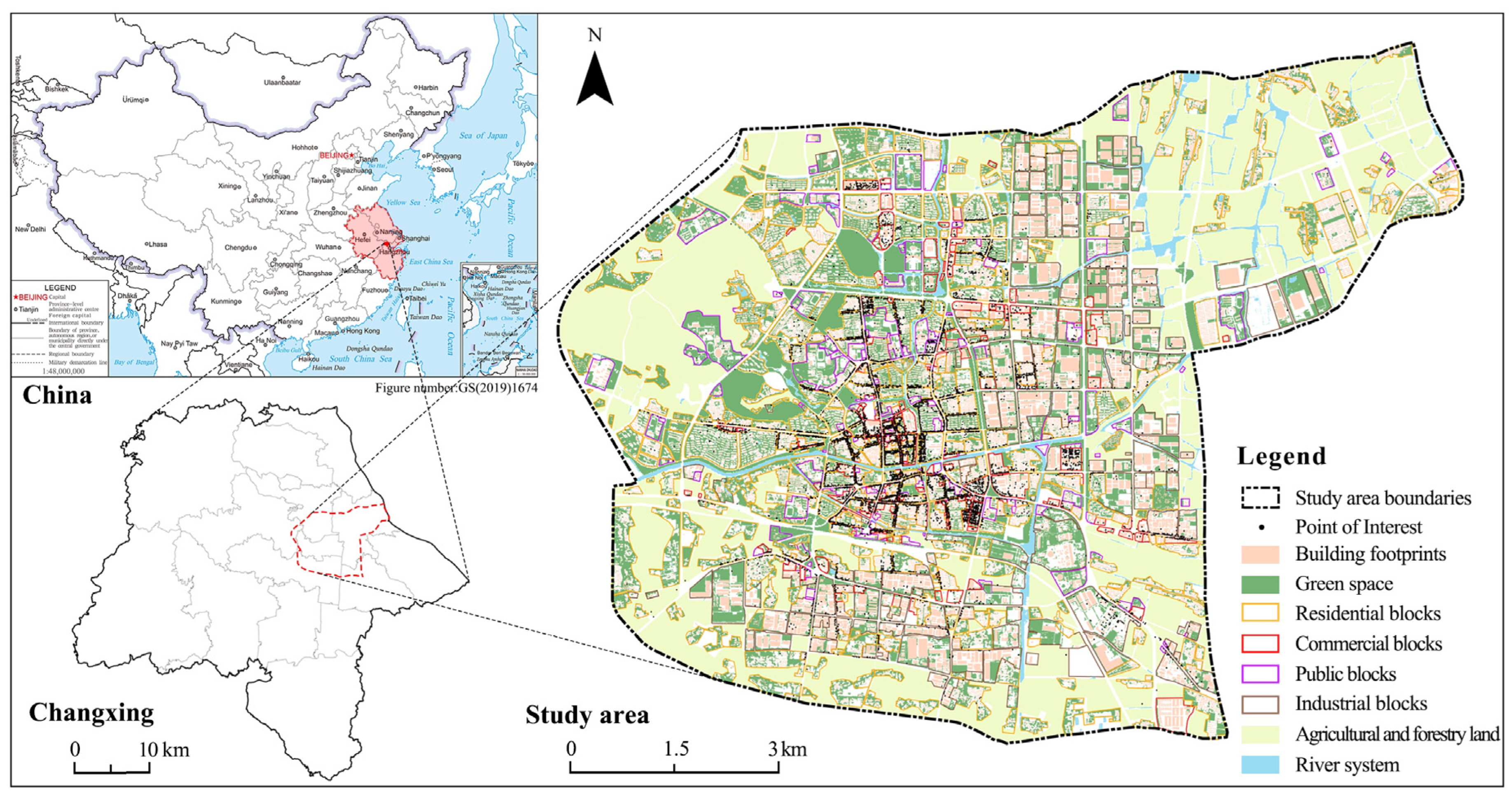
2.1. Study Area and Data Sources

This study focused on the central urban area of Changxing County, Zhejiang Province (Figure 1). At the end of 2018, the central urban area covered an area of 82.51 km², including four streets: Zhicheng Street, Taihu Street, Longshan Street, and Huaxi Street. The population size was approximately 300.000, making it a typical small city. Changxing County is located in the north of Zhejiang Province, on the southwest bank of Taihu Lake, and in the center of the Yangtze River Delta. It has typical climate characteristics of hot summers and cold winters. As one of China’s top 100 counties in terms of economic competitiveness and top 100 in terms of industry, according to the 2010–2017 Changxing County Greenhouse Gas Inventory Report, the level of total carbon emissions and intensity in Changxing County is relatively high, and it faces a severe carbon emission control situation. Simultaneously, the study area serves as the political, economic, and cultural center of Changxing County, with a dense distribution of various elements such as buildings, businesses, population, public service facilities, etc. Therefore, exploring the relationship between density and CICL by taking the central urban area of Changxing County as an example is significantly representative and typical.

This study involved the following data: (1) The Land Use Map of the Central Urban Area of Changxing County: The land use vector map for the year 2018 was provided by the Changxing County Construction Bureau, which displays the area and spatial distribution of different types of blocks in the urban area. (2) Building footprints: Based on the 2018 Changxing County central urban digital elevation map (DEM) data, the area, perimeter, and floor number of buildings of different properties were extracted by classification and then combined with manual correction to obtain complete building information. (3) Green area information: Based on Google’s high-precision historical remote sensing images in 2018 on the Ovi Maps platform, the extraction of green space information on blocks was achieved using the Alibaba DAMO Academy’s AI Earth platform (https://engine-aiearth.aliyun.com, accessed on 8 September 2023). (4) Population data: The population data at the block level in the central urban area in 2018 were provided by the Public Security Bureau of Changxing County. (5) Point of interest (POI): This was obtained based on the Peking University Open Research Data Platform (https://opendata.pku.edu.cn, accessed on 15 September 2023). (6) Energy consumption data: The annual electricity consumption data for block-level land units in 2018 was provided by Changxing County Power Supply Company.

2.2. Quantification of Variables

2.2.1. Quantification of the CICL

In this study, urban construction land primarily refers to residential blocks (RBs), commercial blocks (CBs), and public blocks (PBs). Industrial blocks were not included in this study, mainly due to the fact that the carbon intensity of industrial blocks is more affected by the type of industry, technology level, and energy structure, etc. [33]. This research employed a sampling survey approach to select samples from these three types of urban blocks. The sample sizes of RBs, CBs, and PBs were selected as 106, 49, and 54, respectively, representing 27.3%, 31.6%, and 47.8% of the total number of corresponding blocks. The samples were widely distributed across different regions of the central urban area (Figure 2a), ensuring the representativeness of the samples in terms of quantity and spatial distribution. It is worth noting that the energy consumption of these three types of block accounts for a relatively high proportion of the city’s total energy consumption [34]. Moreover, the electricity consumption of the sampled blocks accounted for over 93% of the total energy consumption during the building operation stage, with most ratios exceeding 99% [14]. These findings were consistent with existing research conclusions [35]. This study used electrical energy consumption to represent the total energy consumption of the building operations. Therefore, based on the annual electricity consumption data of the sampled blocks, carbon emissions were calculated using the carbon emission factor method [36]. The carbon emission intensity for the different block types was determined by the total carbon emissions ratio on that block compared to the block area. Figure 2a illustrates the spatial distribution of the sample blocks; Figure 2b shows the carbon intensity of the blocks expressed in terms of building form.

$$C=e\times f$$

(1)

$$E_c=C/S$$

(2)

where $C$ is the total carbon emissions from the blocks (in kg); $e$ denotes the electricity consumption (in kWh); $f$ is the carbon emission coefficient for electricity (in kgCO₂/kWh); this study used the local carbon emissions per unit of electricity consumption in Changxing, and the value was 0.8463 kgCO₂/kWh; $E_c$ is the carbon emission intensity of the blocks (in kgCO₂/m²); and $S$ is the block area (in m²).

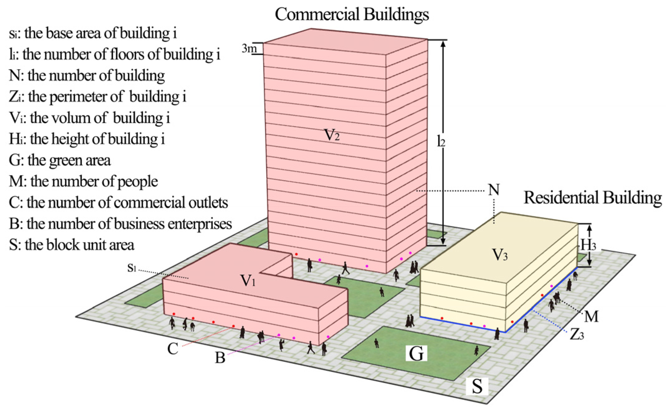
2.2.2. Description and Quantification of Density System

Based on previous research, this paper constructed a comprehensive density measurement system that reflects the distribution characteristics of the physical environment and socioeconomic factors on the blocks (Figure 3). Among them, physical environmental factors (PEFs) mainly refer to artificial environments such as buildings, facilities, and landscapes on the blocks. Factors such as the floor area ratio (FAR), building density (BD) [37], building height (BH) [38], building facade index (BFI) [39], building quantity density (BQD), land use mix density (LMD) [40], building congestion degree (BCD), and green area ratio (GAR) were selected to represent these factors. Considering the diversity of building heights on the blocks, three factors [41,42], namely, the average building height (ABH), maximum building height (MBH), and standard deviation of the building height (SDBH), were selected to describe the building height characteristics accurately. Socioeconomic factors (SEFs) mainly refer to population distribution, economic vitality, and other non-physical environments on the blocks. Three factors, namely, the population density (PD), commercial outlet density (COD), and business enterprise density (BED), were selected to represent the SEFs. Among them, PD represents social factors on the blocks. The density of commercial outlets and business enterprises, as the main body of the city’s tertiary industry, can indicate the level of economic activity on blocks [43]. Commercial outlets mainly include life services, catering, shopping, automobile and motorcycle services, and other commercial types. Business enterprises mainly include corporate enterprises, financial insurance enterprises, and other enterprise types.

Table 1. Description of density system.

Density System		Equation	Indicator Description
Physical Environmental Factors (PEFs)	Floor area ratio (FAR)	$FAR=\frac{{\sum }_{i=1}^N{s}_i{l}_i}{S}$	Reflecting the block development intensity.
	Building density (BD)	$BD=\frac{{\sum }_{i=1}^N{s}_i}{S}$	Reflecting the proportion of the block covered by buildings.
	Average building height (ABH)	$ABH=\frac{{\sum }_{i=1}^N{s}_i{l}_i}{{\sum }_{i=1}^n{s}_i}$	Reflecting the average height of buildings on the block.
	Highest building height (HBH)	$HBH=\max \left(H_i\right)$	Reflecting the maximum building height on the block.
	Standard deviation of building height (SDBH)	$SDBH=\sqrt{\frac{{\sum }_{i=1}^N{\left(H_i-MBF\right)}^2}{N}}$	Reflecting the dispersion and variation in building heights on the block.
	Building facade indicators (BFIs)	$BFI=\frac{{\sum }_{i=1}^N{Z}_i{H}_i}{{\sum }_{i=1}^N{s}_i{l}_i}$	Reflecting the conditions of natural light, landscape, spatial perception, etc., for buildings on the block.
	Building congestion degree (BCD)	$BCD=\frac{{\sum }_{i=1}^N{V}_i}{HBH\ast S}$	Reflecting the proportion of building volumes on the block.
	Land use mix density (LMD)	$LUMD=\frac{{\sum }_{j=1}^m{s}_j{l}_j}{{\sum }_{i=1}^N{s}_i{l}_i}$	Reflecting the degree of mixed block use functionality.
	Building quantity density (BQD)	$BQD=\frac{N}{S}$	Reflecting the quantitative characteristics of buildings on the block.
	Green area ratio (GAR)	$GAR=\frac{G}{S}$	Reflecting the level of green areas on the block.
Socioeconomic Factors (SEFs)	Population density (PD)	$PD=\frac{M}{S}$	Reflecting the characteristics of the population distribution on the block.
	Commercial outlet density (COD)	$COD=\frac{C}{S}$	Reflecting the characteristics of the commercial outlet distribution on the block.
	Business enterprise density (BED)	$BED=\frac{B}{S}$	Reflecting the characteristics of the distribution of business companies on the block.

$s_i$ is the base area of building $i$. $l_i$ is the number of floors of building $i$. $H_i$ is the height of building $i$. $N$ is the number of building types on the block. $Z_i$ is the perimeter of building $i$. The height of each floor in building $i$ is 3 m. $V_i$ is the volume of building $i$. $s_j$ is the area of building $j$ of the j-th type. $m$ is the number of buildings of type $j$. G is the green area. $M$ is the number of people. $C$ is the number of commercial outlets. $B$ is the number of business enterprises. $S$ is the block unit area.

and Figure 3 show the specific descriptions of the density factors.

Table 2. Descriptive statistics of the variables.

Variable	RB				CB				PB
	MEAN	SD	Min	Max	MEAN	SD	Min	Max	MEAN	SD	Min	Max
CICL	22.522	12.079	1.711	59.635	80.190	71.790	1.277	270.547	27.843	30.089	2.135	120.176
FAR	1.227	0.588	0.299	2.855	2.063	1.266	0.639	6.735	0.798	0.389	0.254	1.882
BD	0.256	0.057	0.125	0.409	0.359	0.099	0.164	0.558	0.222	0.091	0.102	0.424
ABH	15.289	9.072	4.665	41.726	18.196	12.371	4.344	64.458	10.772	3.057	4.479	20.056
HBH	29.208	20.790	9.000	96.000	34.714	22.450	9.000	84.000	18.167	8.153	9.000	54.000
SDBH	7.692	7.133	0.722	33.020	12.410	10.927	0.000	50.912	4.798	2.537	0.000	12.096
BFI	1.010	0.266	0.497	1.608	0.573	0.262	0.144	1.358	0.767	0.244	0.323	1.288
BCD	0.051	0.023	0.013	0.106	0.040	0.026	0.006	0.112	0.037	0.024	0.006	0.130
BQD	0.002	0.001	0.000	0.006	0.001	0.001	0.000	0.003	0.001	0.001	0.000	0.003
LMD	0.031	0.045	0.000	0.204	0.057	0.115	0.000	0.445	0.041	0.099	0.000	0.423
GAR	0.321	0.102	0.104	0.638	0.122	0.129	0.000	0.551	0.255	0.188	0.000	0.694
PD	0.251	0.984	0.000	8.902	0.992	1.852	0.000	8.716	0.860	1.557	0.002	8.580
COD	0.001	0.001	0.000	0.006	0.002	0.002	0.000	0.010	0.000	0.001	0.000	0.005
BED	0.000	0.000	0.000	0.002	0.001	0.001	0.000	0.002	0.000	0.001	0.000	0.004

reports descriptive statistics for the dependent variable and all the independent variables. The blocks’ density and carbon emission intensity characteristics are shown in the Supplementary Materials.

2.3. Optimal-Parameters-Based Geographical Detector (OPGD)

A Geodetector is a spatial statistical method used to measure spatial variations, detect explanatory factors, and analyze the interaction relationships between variables [44]. This method has several characteristics, such as not requiring a linear assumption between the dependent and explanatory variables [45], not needing to consider multicollinearity issues with explanatory variables [46], and determining how the interaction between two explanatory variables affects the dependent variable [47]. It also offers more advantages in assessing the impact of explanatory variables compared to principal component analysis and geographically weighted regression [48]. This study employed an OPGD. Compared to a traditional Geodetector, this model does not require manual setting when discretizing continuous variables. Instead, it automatically selects the parameter combination with the highest q-value (classification method and number of intervals) for spatial discretization. The classification method is determined based on statistical rules such as the equal interval, natural interval, quantile range, and geometric interval. The number of intervals is typically set between 3 and 10 [49].

This study employed three components of the model: factor detection, interaction detection, and risk detection. In the factor detection module, the q-value of each continuous factor was calculated under different classification methods and numbers of intervals. The q-value ranges from 0 to 1; a higher q-value indicates a stronger explanatory power of the density factors for the spatial variation in the CICL. Generally, a q-value greater than 0.3 shows a relatively strong driving force on the CICL [50].

$$q=1-\frac{\left({\sum }_{h=1}^L{N}_h{{\sigma }^2}_h\right)}{\left(N{\sigma }^2\right)}=1-\frac{SSW}{SST}$$

(3)

where $h=1\dots L$ is the stratification of the block carbon emission intensity or density factors; $N_h$ and $N$ denote the number of units in layer $h$ and in the total district; ${{\sigma }^2}_h$ and ${\sigma }^2$ are the variance values of the block carbon emission intensity in the $h$ layer and in the total district, respectively; $SST$ is the total sum of squares; and $SSW$ is the within sum of squares.

The interaction detection module compares the q-value of factors X1 and X2 with the interaction q-value (X1∩X2) to quantify the interaction between the two explanatory factors. This evaluation helps to determine whether the factors are mutually weakening, strengthening, or independent. Generally, the results of the interaction detector can be classified into five types: ① nonlinear weakening: q(X1∩X2) < min(q(X1), q(X2)); ② single-factor nonlinear weakening: min(q(X1), q(X2)) < q(X1∩X2) < max(q(X1), q(X2)); ③ dual-factor strengthening: q(X1∩X2) > max(q(X1), q(X2)); ④ independent: q(X1∩X2) = q(X1) + q(X2); and ⑤ nonlinear strengthening: q(X1∩X2) > q(X1) + q(X2). The risk detection module was used to identify the suitable range or type of impact of different density factors on the CICL [51], providing a basis for density factor regulation.

3. Results

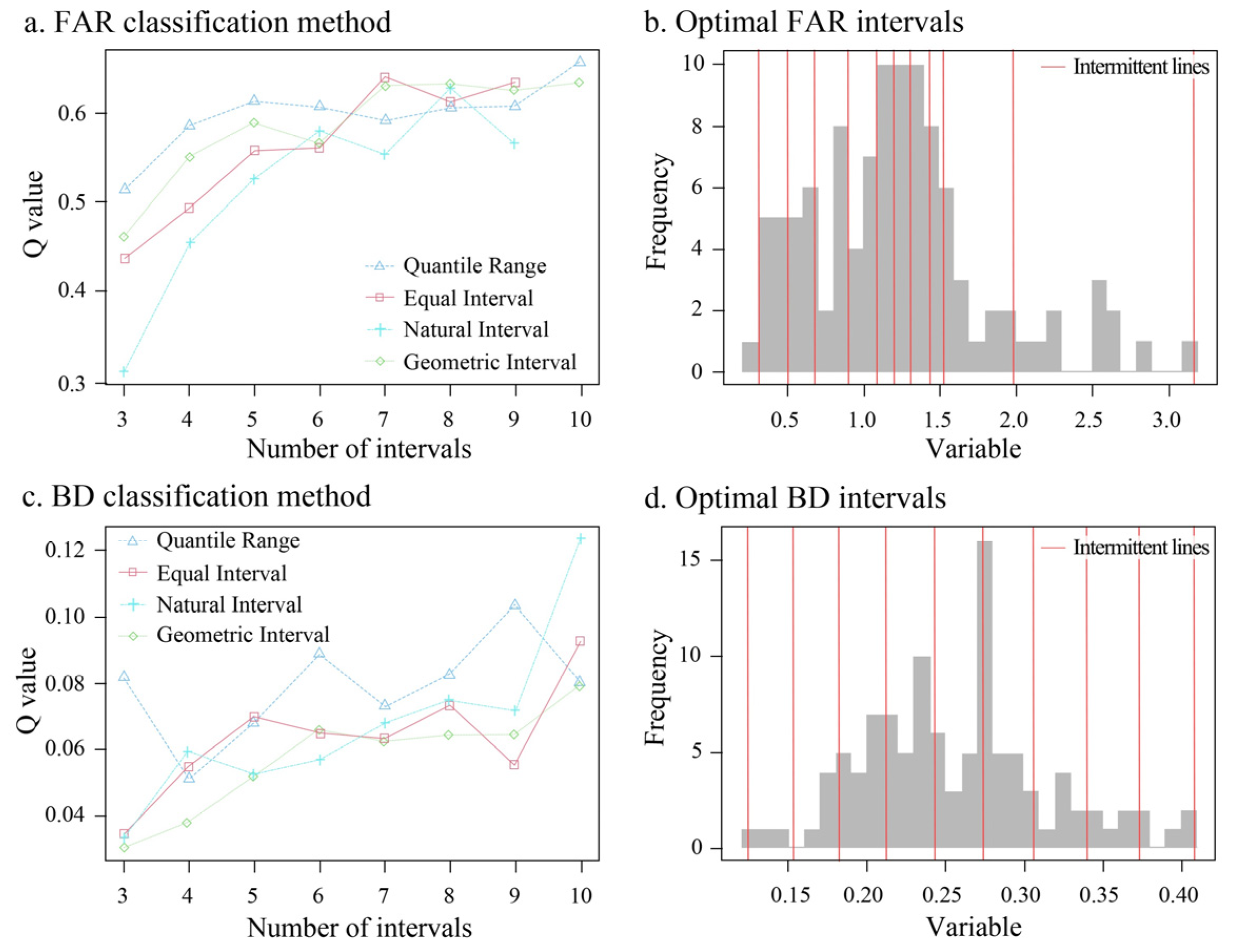
3.1. Discretization Results of Density Factor

Based on the OPGD, the interval number was set to 3–10 during the discretization process of each density factor. Taking the FAR and BD of RB as an example, for the FAR, when the classification method was the quantile range and the number of categories was ten, the q-value was the highest (Figure 4a), so the quantile range was used to divide the FAR into ten categories (Figure 4b). In the same way, the geometric interval was used to divide BD into ten categories (Figure 4c,d). The principle of discretization of the other density factors was the same.

3.2. Analysis of Driving Forces of CIRB

The factor detection results (

Table 3. Single-factor detection results.

Density System		a. CIRB	b. CICB	c. CIPB
PEFs	FAR	0.7086 **	0.5378 **	0.5652 **
	BD	/	/	0.5433 **
	ABH	0.4849 **	0.4902 **	0.3609 **
	HBH	0.5003 **	/	0.3871 *
	SDBH	0.5265 **	0.4088 *	0.5062 **
	BFI	0.3537 **	/	/
	BCD	0.2133 *	/	/
	BQD	0.3428 **	0.3715 *	0.2932 *
	LMD	0.3463 *	/	/
	GR	/	/	0.3780 **
SEFs	PD	0.2345 **	0.4204 *	0.3732 *
	COD	0.3143 **	/	/
	BED	0.2770 *	0.4993 *	0.4541 *

Note: * and ** represent significance at the 0.05 and 0.01 levels, respectively.

, column a) indicated that the other eleven factors passed the significance test except for the BD and GAR. Overall, the single-factor driving force showed that the explanatory power of the PEFs (q: 0.2133–0.7086) was greater than that of the SEFs (q: 0.2345–0.3143). Among them, in the PEFs, the explanatory power of the FAR (0.7086) was the strongest, indicating that the driving effect of land development intensity on the CIRB was very strong. The three indicators reflecting the building height characteristics, namely, the SDBH (0.5265), MBH (0.5003), and ABH (0.4849), all had a substantial impact, highlighting the importance of building height as a driving force for the CIRB. In the SEFs, the COD (0.3143) had a relatively strong explanatory power, reflecting that the distribution of commercial outlets significantly increased the CIRB.

The results of the interaction detection (Figure 5a) indicated that, firstly, in terms of the interaction among the PEFs, the explanatory power after the interaction between the FAR and each factor was significantly enhanced, with an average q-value reaching 0.8169. Notably, the explanatory power was strongest when interacting with the BD, showing a nonlinear enhancement with a q-value of 0.8694. This result indicated that the synergistic effect of the two could explain 86.94% of the CIRB, highlighting the dominant role of the interaction between land development intensity and building coverage on the CIRB. This study also found that the BD showed no correlation in the single-factor detection with the CIRB, but its explanatory power experienced a significant nonlinear enhancement after interacting with the FAR and ABH. This result suggested that the BD only exhibited its driving effect on the CIRB when interacting with other factors. Additionally, the interaction between the FAR and BFI was strong, with a q-value of 0.8626, second only to the maximum q-value, reflecting that the interaction between land development intensity and building form had a relatively strong driving effect on the CIRB. Secondly, in terms of the interaction among the SEFs, the explanatory power of the interaction between various factors performed well. Notably, the interaction between the PD and BED showed a stronger performance, exhibiting a nonlinear enhancement with a q-value of 0.5661. Compared with the interaction of the PEFs, it was evident that the interaction of the SEFs was not the dominant factor in the CIRB. Finally, in terms of the interaction between the PEFs and SEFs, the overall performance of the explanatory power of each factor was enhanced. Among them, the interaction of the FAR with the SEFs and the interaction of the BFI with the SEFs had relatively strong explanatory power for the CIRB, with average q-value of 0.8208 and 0.6595, respectively. Notably, the q-value of the interaction between the FAR and PD reached 0.8575, indicating a strong driving effect of their interaction on the CIRB.

This study found that for the RB, which serves as the primary space for urban residents’ daily life functions, the intensity of its carbon emissions was mainly driven by the PEFs and their interactions. Additionally, the interaction between the PEFs and SEFs also played a significant driving role.

3.3. Analysis of Driving Forces of the CICB

The factor detection results (Table 3, column b) indicated that six factors, including the FAR, ABH, SDBH, BQD, PD, and BED, passed the significance test. Overall, the single-factor driving force showed that the explanatory power of the PEFs (q: 0.3715–0.5378) was greater than that of the SEFs (q: 0.4204–0.4993). In the PEFs, the FAR (0.5378) had the strongest explanatory power. The ABH (0.4902), SDBH (0.4088), and BQD (0.3715) also had a high impact, indicating that the intensity of land development, building height, and quantity characteristics significantly had a significant driving effect on the CICB. In the SEFs, the BED (0.4993) and PD (0.4204) showed a high explanatory power. However, the COD did not exhibit a correlation with the CICB.

The results of the interaction detection (Figure 5b) indicated that, firstly, in terms of the interaction among the PEFs, the explanatory power significantly increased after the interaction among various factors. In particular, the interaction between the FAR, ABH, and SDBH with other factors showed significant enhancement, with average q-value of 0.7036, 0.6947, and 0.6946, respectively. This study also observed that the interaction of the BD with the ABH and the interaction of the BFI with the SDBH exhibited a significant non-linear enhancement, with q-value reaching 0.8540 and 0.8357, respectively. However, the BD and BFI showed no correlation in the factor detection, reflecting that their driving effects on the CICB need to be manifested in interaction with other factors. Secondly, in terms of the interaction among the SEFs, the interaction effects of various factors performed well in explaining the CICB, with an average q-value of 0.6208. Notably, the interaction between the PD and BED showed slightly better explanatory power and a linear enhancement, with a q-value of 0.7254. Finally, in terms of the interaction between the PEFs and SEFs, the explanatory power significantly increased, especially the interaction between the FAR and SEFs, with an average q-value of 0.8713. In particular, the interaction with the COD exhibited the strongest explanatory power and a non-linear enhancement, with a q-value of 0.9127. This result indicated that the synergistic effect of the two could explain 91.27% of the CICB, clearly highlighting the decisive role of land development intensity and the distribution of commercial points in determining the CICB. Notably, the COD showed no correlation in the single-factor detection, but its impact became significantly manifest in the interaction with factors such as the FAR and SDBH. Additionally, the explanatory power of the interaction between the FAR and BED, as well as the PD and ABH, reached q-value of 0.8842 and 0.8420, respectively, which were second only to the highest q-value.

The above research results fully demonstrated that for the CB, which serves as the space to support the economic development of the service industry, its carbon emission intensity resulted from the combined effects of the PEFs and SEFs. At the same time, the interaction among the PEFs also played an essential driving role.

3.4. Analysis of Driving Forces of the CIPB

The factor detection results (Table 3, column c) indicated that the other nine factors passed the significance test except for the BFI, BCD, LMD, and COD. Overall, the single-factor driving force showed that the explanatory power of the PEFs (q: 0.2932–0.5652) was greater than that of the SEFs (q: 0.3732–0.4541). Among them, in the PEFs, the explanatory power of the FAR (0.5652) was the highest, and the impact of the BD (0.5433) and SDBH (0.5062) was also significant. This result indicated that the intensity of land development, building coverage, and variations in building height had a significant driving effect on the CIPB. In the SEFs, the explanatory power of the BED (0.4541) was relatively strong, indicating a significant driving effect of the distribution of business enterprises on carbon emissions, and the impact of the PD (0.3732) was also significant.

The results of the interaction detection (Figure 5c) indicated that, firstly, in terms of the interaction among the PEFs, the explanatory power of the FAR, BD, and SDBH after interaction with various factors performed well, with average q-value of 0.7035, 0.7041, and 0.6853, respectively. Among them, the interactions between the FAR and MBH and between the MBH and BCD showed relatively strong explanatory power with linear and nonlinear enhancements, respectively, and with q-value of 0.8326 and 0.8067. Secondly, in terms of the interaction among the SEFs, the explanatory power of each factor’s interaction was moderate, with average q-value of 0.5078. The interaction between the PD and BED showed a slightly better explanatory power. It showed a linear enhancement with a q-value of 0.6366, indicating that the interaction of the SEFs was not the dominant factor in the CIPB. Finally, in terms of the interaction between the PEFs and SEFs, the overall explanatory power of their interactions was quite strong. In particular, the interaction between the FAR and PD exhibited the strongest explanatory power and a showed significant nonlinear enhancement, with a q-value of 0.9396. This result indicated that the synergistic effect of the two could explain 93.96% of the CIPB, highlighting the decisive role of land development intensity and population distribution in determining the CIPB. It is worth noting that during the individual factor detection, there was no correlation between the COD, BFI, and CIPB. However, after considering the interaction between the COD and FAR and the interaction between the PD and SDBH, their explanatory power significantly increased, showing a significant nonlinear strengthening effect, with q-value of 0.9220 and 0.8337, respectively, ranking just below the highest value.

This study found that for the PB, which serves as a space that undertakes urban social management and service functions, its carbon emission intensity resulted from the interaction between the PEFs and SEFs. Additionally, the interaction among the PEFs also played a significant role.

4. Discussion

As a key indicator related to the sustainable development of cities [8], density has gained growing attention in academic circles regarding its impact on the CICL. It is worth noting that different land use types serve different functions in the urban operation process, leading to significant differences in carbon emissions regarding generation methods, intensity, and other aspects. These differences also result in substantial variations in the effects of density factors and their interactions on the land carbon emission intensity. However, the OPGD effectively detected the impact of the PEFs and SEFs and their interactions on the carbon emission intensity in different block types. Understanding the relationship between the urban physical environment, socioeconomic characteristics, and carbon emissions is significant for implementing effective carbon reduction actions [52].

4.1. Analysis of Single-Factor Driving Forces on CICL

From the perspective of single-factor analysis, at least one factor from the density system consisting of thirteen factors constructed in this study was correlated with either the CIRB, CICB, or CIPB, confirming the rationality of selecting density indicators. Among these factors, the FAR, ABH, SDBH, BQD, PD, and BED played a driving role in all three types of CICL. Furthermore, the overall impact of the density factors on the carbon emission intensity in the different land uses revealed that the PEFs had a stronger influence than the SEFs. Among them, the FAR exhibited the strongest impact, affirming its dominant role in driving carbon emission intensity, which aligns with previous studies [53,54].

For other density factors, previous research has mainly focused on the relationship between residential land density indicators and carbon emissions, with differences primarily observed in terms of building density [28,55]. As density is a quantitative indicator that describes the urban form and has significant three-dimensional characteristics, this study aimed to further clarify the relationship between the building density (BD) and the CICL by analyzing the spatial form of blocks. First, based on Table 2, we extracted and compared the SD values reflecting the dispersion of the density indicators (Figure 6). We found that three indicators reflecting the building height on construction land, namely, the ABH, HBH, and SDBH, had very high discretization levels. Additionally, the variation in the building height on the RB and CB was significantly greater than that on the PB, indicating that the three-dimensional spatial diversity of the RB and CB was much higher than that of the PB, suggesting a certain level of convergence in the spatial form of the PB. When we selected three typical blocks separately from the RB and CB, with similar levels of BD, we observed significant differences in the spatial forms of the same block type, representing three common spatial patterns in cities: high-rise, multi-story, and low-rise buildings. Figure 7 clearly demonstrates the differences in the spatial patterns of the blocks at similar levels of BD in the RB and CB. We found that the carbon emission intensity increased for the selected RB units as the FAR and ABH increased. However, due to the differences in the three-dimensional spatial form (Figure 7a), the BD remained unchanged, indicating no correlation between the BD and CIRB. This finding was similarly observed in the CB (Figure 7b). However, the significant driving effect of the interaction of these factors on the CICL indicated that the influence of the BD may be mediated, meaning that the driving impact of the BD needs to be manifested significantly through interactions with factors such as the FAR and ABH. The convergence of the three-dimensional spatial form on the PB also resulted in a correlation between the BD and CIPB. Overall, the spatial form of specific land types affects the relationship between density factors and the CICL. This result aligns with existing research conclusions that “different community forms, such as BD and building form, have varying effects on residential energy consumption” [56,57]. This study also discovered that this characteristic applies to other land types.

Regarding the SEFs, there were apparent differences in their impact on the carbon emission intensity of the different land types. For the CIRB, the strongest driving factor was the COD, highlighting the positive influence of the distribution of commercial and service facilities on the carbon emission intensity in this block type. However, some studies have also found that the COD has an inhibitory effect on transport-related carbon emissions [58,59]. As for the CICB and CIPB, the strongest driving factor was the BED, indicating that businesses had a strong promoting effect on the carbon emission intensity in these block types.

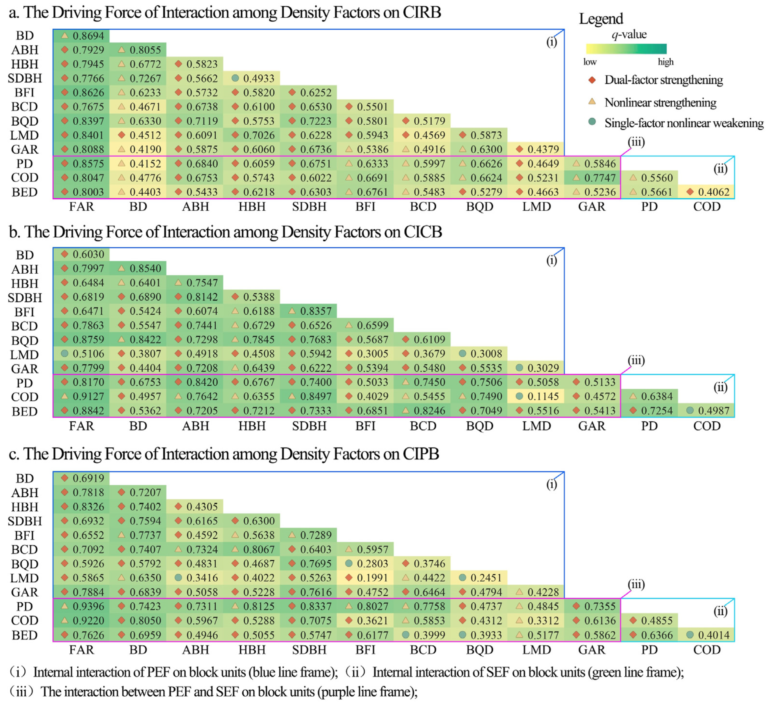
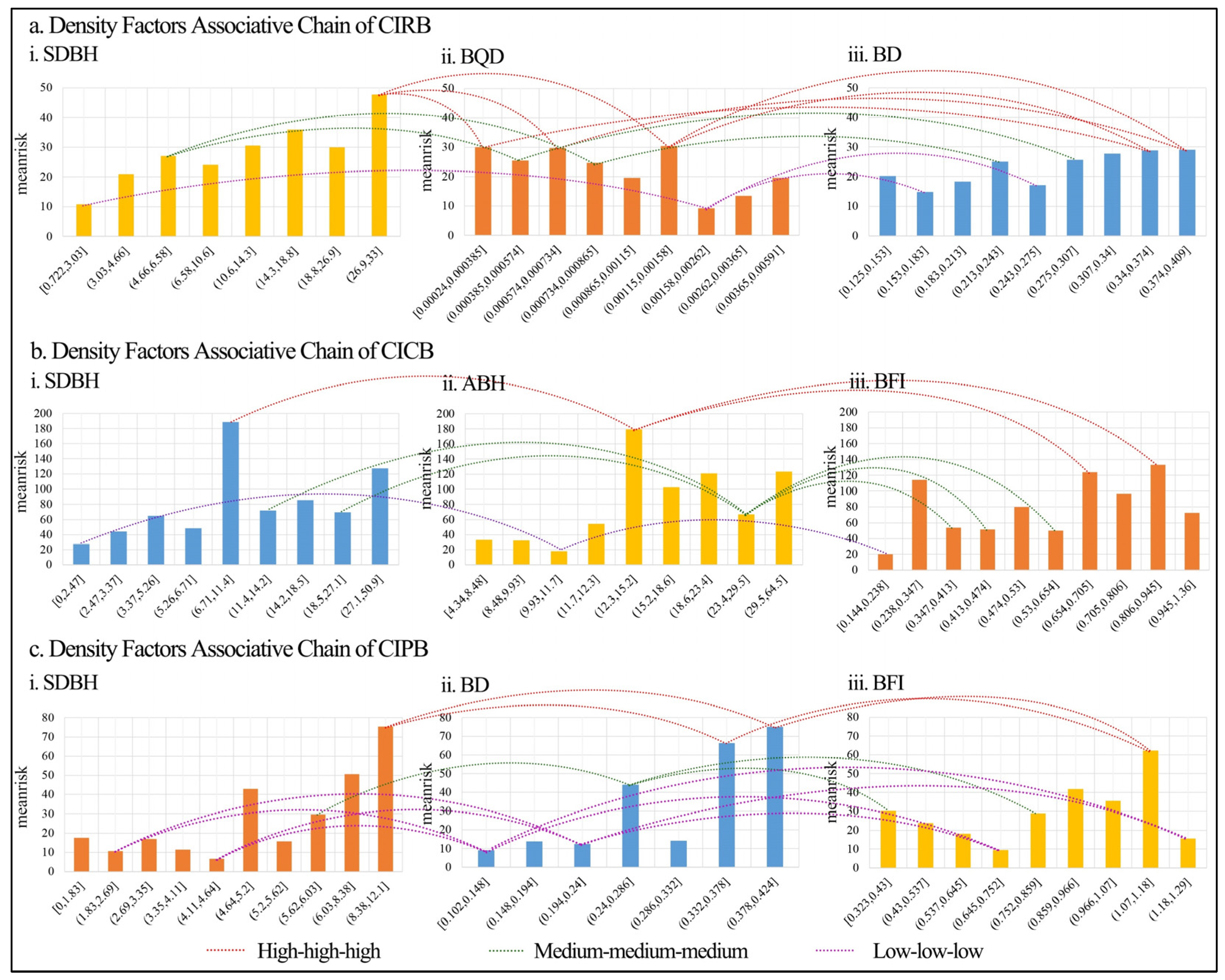
4.2. Analysis of Factor Interaction Driving Forces on the CICL

From the results of the factor interactions, the explanatory power of the interaction of the FAR with the BD for the CIRB, the interaction of the AR with the COD for the CICB, and the interaction of the FAR with the PD for the CIPB were 0.8694, 0.9127, and 0.9396, respectively. This result clarified the necessity of conducting carbon emission research from the perspective of density. We also found that the strongest explanatory power for the carbon emission intensity in the three block types was the combination of the FAR and other factors, and they all exhibited a nonlinear enhancement. It is worth noting that the factors interacting with the FAR adequately reflect the characteristics of the different block types. For example, the interaction between the FAR and COD exhibited the strongest explanatory power for the CICB. In this case, the FAR reflects the intensity of land development, while the COD, as the primary business format, reflects the level of economic activity in the service industry in the CB. Furthermore, combined with the factor detection results, we found that a specific density factor had an impact or a high degree of impact on the CICL, and its influence was not necessarily reflected in the interaction of factors. Some factors only exhibited a more significant impact after interacting with others. For example, the BD showed no correlation with the CIRB, but its interaction with the FAR had the strongest driving force, suggesting that when the level of FAR is determined for a given RB, the BD determines the distribution of the floor area in the block, thereby influencing the formation of wind, thermal, and light environments in the block [60], which, in turn, affects the level of the CIRB.

The above conclusions clearly indicate that the CICL results from the synergistic effects of multiple density factors. The nonlinear characteristics exhibited by the factor interactions align with the conclusion emphasized in previous studies that “the influence of density on carbon emissions is nonlinear and requires the analysis of other socioeconomic factors” [25]. This finding also reflects the limitations of predicting land carbon emissions based solely on individual physical environment or socioeconomic factors, such as POI data [61] and population density [62]. This study provides a basis for exploring carbon emission predictions and simulations based on multi-source data [63,64]. At the same time, it implies that when formulating carbon emission control policies and measures, urban planners should consider the interactions among various factors based on the differences in land use types rather than simply relying on a single density factor as the sole control criterion.

4.3. Policy Implications

Based on the OPGD analysis results, this paper attempted to propose a coordinated spatial planning and control method for carbon emission intensity in different block types. It is important to note that in order to ensure the realization of socioeconomic benefits for construction land, it is not feasible to simply suppress the carbon emission intensity by reducing the FAR. Therefore, by comparing the explanatory power of the two-by-two interactions of multiple density factors on the carbon emission intensity of blocks, this study extracted an associative chain covering multiple density factors for RBs, CBs, and PBs, respectively. Following this, an appropriate interval value for the density factor in the associative chain was specified based on the risk detection results. The results of the risk detection of some density factors on the CIRB, CICB, and CIPB are partially presented in the bar charts in Figure 8. Taking the RB as an example, Figure 8a demonstrates the risk detection results of the three factors SDBH, BQD, and BD, whereas Figure 8(ai) demonstrates the average CIRB corresponding to different numbers of intervals when the number of intervals of SDBH values was 8. The curves in Figure 8a show a degree of consistency in the average carbon intensity of the SDBH, BQD, and BD factors at different interval values, i.e., high–high–high and low–low–low. Based on this correspondence, this study determined the appropriate values of the SDBH, BQD, and BD.

For the RB, the three factors in the association chain “BD–BQD–SDBH” exhibited a relatively high explanatory power through pairwise interactions (Figure 8a), with an average q-value of 0.6940. Therefore, while ensuring the intensity of land development, focusing on appropriately increasing the number of buildings, reducing the building coverage, and minimizing the difference in height between individual buildings can effectively reduce the CIRB. The optimal solution is to control the BQD within the range of (0.00158, 0.00262], the SDBH within the range of (0.722, 3.03], and the BD within the range of (0.153, 0.183] or (0.243, 0.275]. Similarly, for the CB, the association chain consisted of “ABH–SDBH–BFI” (Figure 8b), with an average q-value of 0.7530. Therefore, focusing on appropriately reducing the height difference between individual buildings by lowering the average height and adjusting the aspect ratio of buildings can effectively reduce the CICB. Considering the higher intensity of CB development, the optimal solution would be to control the ABH within the range of (23.4, 29.5], the SDBH within the range of (18.5, 27.1], and the BFI within the range of (0.53, 0.654]. For the PB, the association chain was “BFI–BD–SDBH” (Figure 8c), with an average q-value of 0.7540. Hence, focusing on reducing the building coverage appropriately, combining it with minimizing the difference in height between individual buildings, and adjusting the aspect ratio of buildings can help lower the CIPB. Considering the higher intensity of PB development, an optimal solution could be to control the BD within the range of (0.286, 0.332], the SDBH within the range of (5.2, 5.62], and the BFI within the range of (0.537, 0.752].

4.4. Limitations and Future Outlook

This study investigated the impact of density indicators on the CICL. However, it has the following limitations and the possibility of further research: Firstly, considering the dynamic evolution of urban density, future studies could examine the impact of density changes on the carbon intensity of a site over a more extended period in conjunction with technological advances, policy changes, or economic shifts. This research would contribute to spatial planning and guiding urban spaces toward a more low-carbon direction. Secondly, this study only focused on the central urban area of Changxing County. The research findings may be limited to providing insights into the coordinated control of carbon emissions in small county-level cities in the Yangtze River Delta region. Future studies could select more small cities from different areas to investigate the differences in the impact of density factors on the intensity of land carbon emissions. Lastly, this study represented the total energy consumption in a block using its electricity consumption. There may still be some discrepancies compared to actual data. Future research could collect more comprehensive energy consumption data.

5. Conclusions

Based on multiple data sources such as energy consumption, remote sensing, and POI in the urban block units of Changxing County, this study constructed a density system that reflects the physical environment and socioeconomic characteristics of construction land. By employing an OPGD and selecting the best discretization method and interval count as the optimal combination of parameters to convert the continuous density factor into a discrete factor, this study investigated the effects and interactions of density factors on the CIRB, CICB, and CIPB. The main conclusions are as follows: (1) Regarding the single-factor analysis, at least one factor from the density system consisting of thirteen factors constructed in this study was related to either the CIRB, CICB, or CIPB. Among these factors, the FAR, ABH, SDBH, BQD, PD, and BED played a driving role in all three types of CICL. Additionally, the degree of influence of the different density factors on the carbon emission intensity was closely related to the land use type and its three-dimensional spatial morphology. Furthermore, the explanatory power of the PEFs for the carbon emission intensity in the three types of construction land was stronger than that of the SEFs, with the FAR exhibiting the strongest influence. (2) Regarding the interaction analysis, the CICL resulted from the interaction of multiple density factors. The interactions between the FAR and BD, the FAR and COD, and the FAR and PD demonstrated non-linear enhancements in their explanatory power for the CIRB, CICB, and CIPB, respectively. Additionally, this study found that the factors interacting with the FAR adequately reflected the characteristics of the different types of construction land. However, when combining the results of the single-factor analysis, we found that a specific density factor had an impact or a high degree of impact on the CICL, and its influence was not necessarily reflected in the interaction of factors. Some factors only exhibited a more significant impact after interacting with others. (3) Based on the results of the OPGD analysis, by comparing the explanatory power of the pairwise interactions among multiple factors, a correlated chain encompassing the interactions of multiple density factors was extracted for the CIRB, CICB, and CIPB, respectively. They respectively corresponded to the following three chains: “BD–BQD–SDBH”, “ABH–SDBH–BFI”, and “BFI–BD–SDBH”.

The above results indicated that the OPGD effectively assessed the impact of different density factors and their interactions on the CICL. The research findings can also provide valuable decision support for urban planners in considering the comprehensive effects of density factors and promoting the development of low-carbon and sustainable urban spaces.

References

1. Creutzig, F.; Baiocchi, G.; Bierkandt, R.; Pichler, P.P.; Seto, K.C. Global typology of urban energy use and potentials for an urbanization mitigation wedge. Proc. Natl. Acad. Sci. USA 2015, 112, 6283–6288. [Google Scholar] [CrossRef]
2. Intergovernmental Panel on Climate Change. Climate Change 2014 Mitigation of Climate Change; Cambridge University Press: Cambridge, UK, 2015; p. 147. [Google Scholar]
3. Parry, I.W.H.; Williams, R.C.; Goulder, L.H. When Can Carbon Abatement Policies Increase Welfare? The Fundamental Role of Distorted Factor Markets. J. Environ. Econ. Manag. 1999, 37, 52–84. [Google Scholar] [CrossRef]
4. Jin, T.; Yang, J.; Wang, D. From Urban Density Zoning to Form-based Zoning: Evolution and Demonstration. Urban Plan. Forum 2018, 4, 34–40. [Google Scholar]
5. Zou, B. From Physical Expansion to Built-up Area Improvement: Shenzhen Master Plan Transition Forces and Paths. Planners 2013, 29, 5–10. [Google Scholar]
6. Ge, C.; Zhang, Y.; Li, H.; Guo, Z.; Cai, Y.; Zhao, C.; Liu, X. A New Path toward Governance Transition in Territorial Spatial Planning: The Case of Ningbo. Urban. Plan Forum. 2022, S2, 241–246. [Google Scholar] [CrossRef]
7. Krehl, A.; Siedentop, S.; Taubenböck, H.; Wurm, M. A Comprehensive View on Urban Spatial Structure: Urban Density Patterns of German City Regions. ISPRS Int. J. Geo-Inf. 2016, 5, 76. [Google Scholar] [CrossRef]
8. Yang, J.; Shi, Y. The Evolution and Prospect of Density Research in the Context of Urban Planning. Urban. Plan. Int. 2023, 38, 1–7. [Google Scholar] [CrossRef]
9. Churchman, A. Disentangling the Concept of Density. J. Plan. Lit. 1999, 13, 389–411. [Google Scholar] [CrossRef]
10. Berghauser, P.; Haupt, P.M. Spacemate: The Spatial Logic of Urban Density; DUP Science: Dares Salaam, Tanzania, 2004. [Google Scholar]
11. Dongsheng, H.; Jia, M.; Yi, L.; Yimeng, S.; Long, C.; Ye, L. Urban greenery mitigates the negative effect of urban density on older adults’ life satisfaction: Evidence from Shanghai, China. Cities 2022, 124, 103607. [Google Scholar]
12. Hui, S.C.M. Low energy building design in high density urban cities. Renew. Energy 2001, 24, 627–640. [Google Scholar] [CrossRef]
13. Alvarez Palau, E.; Solanas, J. Urban Growth and Long-Term Transformations in Spanish Cities Since the Mid-Nineteenth Century: A Methodology to Determine Changes in Urban Density. Sustainability 2019, 11, 6948. [Google Scholar] [CrossRef]
14. Zhang, X.; Yan, F.; Liu, H.; Qiao, Z. Towards low carbon cities: A machine learning method for predicting urban blocks carbon emissions (UBCE) based on built environment factors (BEF) in Changxing City, China. Sustain. Cities Soc. 2021, 69, 102875. [Google Scholar] [CrossRef]
15. Dong, Q.; Huang, Z.; Zhou, X.; Guo, Y.; Scheuer, B.; Liu, Y. How building and street morphology affect CO2 emissions: Evidence from a spatially varying relationship analysis in Beijing. Build. Environ. 2023, 236, 110258. [Google Scholar] [CrossRef]
16. Ye, H.; He, X.Y.; Song, Y.; Li, X.; Zhang, G.; Lin, T.; Xiao, L. A sustainable urban form: The challenges of compactness from the viewpoint of energy consumption and carbon emission. Energy Build. 2015, 93, 90–98. [Google Scholar] [CrossRef]
17. Qin, H.; Huang, Q.; Zhang, Z.; Lu, Y.; Li, M.; Xu, L.; Chen, Z. Carbon dioxide emission driving factors analysis and policy implications of Chinese cities: Combining geographically weighted regression with two-step cluster. Sci. Total Environ. 2019, 684, 413–424. [Google Scholar] [CrossRef]
18. Ma, M.; Rozema, J.; Gianoli, A.; Zhang, W. The Impacts of City Size and Density on CO2 Emissions: Evidence from the Yangtze River Delta Urban Agglomeration. Appl. Spat. Anal. Policy 2022, 15, 529–555. [Google Scholar] [CrossRef]
19. Tian, D.; Yang, S.; Guan, C.; Li, Y. Correlation between Urban Spatial Agglomeration and Residents’ Household Carbon Emissions: An Analysis Based on the Data of 110 Chinese Cities. City Plan. Rev. 2023, 47, 76–85. [Google Scholar]
20. Al-Mulali, U. Factors affecting CO2 emission in the Middle East: A panel data analysis. Energy 2012, 44, 564–569. [Google Scholar] [CrossRef]
21. Li, Z.; Wu, H.; Wu, F. Impacts of urban forms and socioeconomic factors on CO2 emissions: A spatial econometric analysis. J. Clean. Prod. 2022, 372, 133722. [Google Scholar] [CrossRef]
22. Zhang, Q.; Yang, J.; Sun, Z.; Wu, F. Analyzing the impact factors of energy-related CO2 emissions in China: What can spatial panel regressions tell us? J. Clean. Prod. 2017, 161, 1085–1093. [Google Scholar] [CrossRef]
23. Liddle, B. Urban density and climate change: A STIRPAT analysis using city-level data. J. Transp. Geogr. 2013, 28, 22–29. [Google Scholar] [CrossRef]
24. Gudipudi, R.; Fluschnik, T.; Ros, A.G.C.; Walther, C.; Kropp, J.P. City density and CO2 efficiency. Energy Policy 2016, 91, 352–361. [Google Scholar] [CrossRef]
25. Chen, F.; Shen, S.; Li, Y.; Xu, H. Impact of urban density on spatial carbon performance: A case study of Shanghai. Urban. Probl. 2022, 96–103. [Google Scholar] [CrossRef]
26. Resch, E.; Bohne, R.A.; Kvamsdal, T.; Lohne, J. Impact of Urban Density and Building Height on Energy Use in Cities. Energy Procedia 2016, 96, 800–814. [Google Scholar] [CrossRef]
27. Quan, S.J.; Economou, A.; Grasl, T.; Yang, P.P. Computing Energy Performance of Building Density, Shape and Typology in Urban Context. Energy Procedia 2014, 61, 1602–1605. [Google Scholar] [CrossRef]
28. Wang, W.; Li, J. Correlation between Residential Density and Carbon Emissions Caused by Household Energy Consumption: A Case Study on Caoyang Xincun, Shanghai. City Plan. Rev. 2017, 41, 83–91. [Google Scholar]
29. Xu, L.; Du, H.; Zhang, X. Driving Forces of Carbon Dioxide Emissions in China’s Cities: An Empirical Analysis Based on the Geodetector Method. J. Clean. Prod. 2020, 287, 125169. [Google Scholar] [CrossRef]
30. Jiang, X.T.; Wang, Q.; Li, R. Investigating factors affecting carbon emission in China and the USA: A perspective of stratified heterogeneity. J. Clean. Prod. 2018, 199, 85–92. [Google Scholar] [CrossRef]
31. Long, Z.; Zhang, Z.; Liang, S.; Chen, X.; Yang, T. Spatially explicit carbon emissions at the county scale. Resour. Conserv. Recycl. 2021, 173, 105706. [Google Scholar] [CrossRef]
32. Zhao Min, T.X. The Economical Principles of Urban Development and Urban Planning; Higher Education Press: Beijing, China, 2001. [Google Scholar]
33. Hongtao, J.; Jian, Y.; Bin, Z.; Danqi, W.; Xinyuan, L.; Yi, D.; Ruici, X. Industrial Carbon Emission Distribution and Regional Joint Emission Reduction: A Case Study of Cities in the Pearl River Basin, China. Chin. Geogr. Sci. 2024, 34, 210–229. [Google Scholar]
34. Shahrokni, H.; Levihn, F.; Brandt, N. Big meter data analysis of the energy efficiency potential in Stockholm’s building stock. Energy Buildings 2014, 78, 153–164. [Google Scholar] [CrossRef]
35. Dean, B.; Dulac, J.; Petrichenko, K.; Graham, P. Towards Zero-Emission Efficient and Resilient Buildings: Global Status Report; Global Alliance for Buildings and Construction (GABC): Paris, France, 2016. [Google Scholar]
36. Houghton, J.T. Revised 1996 IPCC Guidelines for National Greenhouse Gas Inventories; IPCC Task Force on National Greenhouse Gas Inventories: Geneva, Switzerland, 1996. [Google Scholar]
37. Cao, Q.; Luan, Q.; Liu, Y.; Wang, R. The effects of 2D and 3D building morphology on urban environments: A multi-scale analysis in the Beijing metropolitan region. Build. Environ. 2021, 192, 107635. [Google Scholar] [CrossRef]
38. Wu, W.; Li, L.; Li, C. Seasonal variation in the effects of urban environmental factors on land surface temperature in a winter city. J. Clean. Prod. 2021, 299, 126897. [Google Scholar] [CrossRef]
39. Uytenhaak, R. Cities Full of Space: Quality of Density; Nai010 Publishers: Rotterdam, The Netherlands, 2009. [Google Scholar]
40. Nes, A.V.; Pont, M.B.; Mashhoodi, B. Combination of Space syntax with spacematrix and the mixed use index: The Rotterdam South test case. In Proceedings of the 8th International Space Syntax Symposium, Santiago, Chile, 3–6 January 2012. [Google Scholar]
41. Zhang, P.; Hu, Y.; Xiong, Z. Extraction of Three-Dimensional Architectural Data from QuickBird Images. J. Indian Soc. Remote 2014, 42, 409–416. [Google Scholar] [CrossRef]
42. Jiang, L.; Liu, S.; Liu, L.; Liu, C. Revealing the spatiotemporal characteristics and drivers of the block-scale thermal environment near a large river: Evidences from Shanghai, China. Build. Environ. 2022, 226, 109728. [Google Scholar] [CrossRef]
43. Lu, C.; Pang, M.; Zhang, Y.; Li, H.; Cheng, W. Mapping Urban Spatial Structure Based on POI (Point of Interest) Data: A Case Study of the Central City of Lanzhou, China. Int. J. Geo-Inf. 2020, 9, 92. [Google Scholar] [CrossRef]
44. Chen, C.; Bi, L. Study on spatio-temporal changes and driving factors of carbon emissions at the building operation stage- A case study of China. Build. Environ. 2022, 219, 109147. [Google Scholar] [CrossRef]
45. Yang, J.; Song, C.; Yang, Y.; Xu, C.; Guo, F.; Xie, L. New method for landslide susceptibility mapping supported by spatial logistic regression and GeoDetector: A case study of Duwen Highway Basin, Sichuan Province, China. Geomorphology 2018, 324, 62–71. [Google Scholar] [CrossRef]
46. Luo, L.; Mei, K.; Qu, L.; Zhang, C.; Chen, H.; Wang, S.; Di, D.; Huang, H.; Wang, Z.; Xia, F. Assessment of the Geographical Detector Method for investigating heavy metal source apportionment in an urban watershed of Eastern China. Sci. Total Environ. 2019, 653, 714. [Google Scholar] [CrossRef]
47. Wang, J.-F.; Zhang, T.-L.; Fu, B.-J. A measure of spatial stratified heterogeneity. Ecol. Indic. Integr. Monit. Assess. Manag. 2016, 67, 250–256. [Google Scholar] [CrossRef]
48. Shrestha, A.; Luo, W. Analysis of Groundwater Nitrate Contamination in the Central Valley: Comparison of the Geodetector Method, Principal Component Analysis and Geographically Weighted Regression. ISPRS Int. J. Geo-Inf. 2017, 6, 297. [Google Scholar] [CrossRef]
49. Zhang, R.; Chen, Y.; Zhang, X.; Fang, X.; Ma, Q.; Ren, L. Spatial-Temporal Pattern and Driving Factors of Flash Flood Disasters in Jiangxi Province Analyzed by Optimal Parameters-Based Geographical Detector. Geogr. Geo-Inf. Sci. 2021, 37, 72–80. [Google Scholar]
50. Chen, G.; Luo, J.; Zhang, C.; Jiang, L.; Tian, L.; Chen, G. Characteristics and Influencing Factors of Spatial Differentiation of Urban Black and Odorous Waters in China. Sustainability 2018, 10, 4747. [Google Scholar] [CrossRef]
51. Wang, J.; Xu, C. Geodetector: Principle and prospective. Acta Geogr. Sin. 2017, 72, 116–134. [Google Scholar]
52. Wu, D.; Lin, J.C.; Oda, T.; Kort, E.A. Space-based quantification of per capita CO2 emissions from cities. Environ. Res. Lett. 2020, 15, 035004. [Google Scholar] [CrossRef]
53. Rosenfeld, H. Mitigation of Urban Heat Islands: Material, Utility Programs, Updates. Enegy Build. 1995, 22, 255–265. [Google Scholar] [CrossRef]
54. Anderson, J.E.; Wulfhorst, G.; Lang, W. Energy analysis of the built environment—A review and outlook. Renew. Sustain. Energy Rev. 2015, 44, 149–158. [Google Scholar] [CrossRef]
55. Wei, W.; Yan, S.; Zaisheng, H.; Yihua, L. Research of the Influence of Community Form on residential Energy Consumption: A Case Study on Ningbo City. Urban Dev. Stud. 2018, 25, 15–20. [Google Scholar]
56. Rode, P.; Keim, C.; Robazza, G.; Viejo, P.; Schofield, J. Cities and energy: Urban morphology and residential heat-energy demand. Environ. Plan. B: Plan. Des. 2014, 41, 138–162. [Google Scholar] [CrossRef]
57. Wilson, B. Urban form and residential electricity consumption: Evidence from Illinois, USA. Landsc. Urban Plan. 2013, 115, 62–71. [Google Scholar] [CrossRef]
58. Krizek, K.J. Residential Relocation and Changes in Urban Travel. J. Am. Plan. Assoc. 2003, 69, 265–281. [Google Scholar] [CrossRef]
59. Peijun, R.; Lijun, Z.; Yaochen, Q.; Yang, L.I.; Zhicheng, Z. Impact of built environment on carbon emissions from daily travel of urban residents: A case study of 248 residential areas in Kaifeng. Geogr. Res.-Aust. 2019, 38, 1464–1480. [Google Scholar]
60. Jiyu, D. Research on Urban Spatial Form of Cbd Based on Microclimate Analysis—A Case Study of Nanjing. Ph.D. Thesis, Southeast University, Nanjing, China, 2019. [Google Scholar]
61. Zheng, Y.; Du, S.; Zhang, X.; Bai, L.; Wang, H. Estimating carbon emissions in urban functional zones using multi-source data: A case study in Beijing. Build. Environ. 2022, 212, 108804. [Google Scholar] [CrossRef]
62. Olivier, J.G.J.; Van Aardenne, J.A.; Dentener, F.J.; Pagliari, V.; Ganzeveld, L.N.; Peters, J.A.H.W. Recent trends in global greenhouse gas emissions: Regional trends 1970–2000 and spatial distribution of key sources in 2000. Environ. Sci. 2005, 2, 81–99. [Google Scholar] [CrossRef]
63. Yoshida, T.; Yamagata, Y.; Murakami, D. Energy demand estimation using quasi-real-time people activity data. Energy Procedia 2019, 158, 4172–4177. [Google Scholar] [CrossRef]
64. Chuai, X.; Feng, J. High resolution carbon emissions simulation and spatial heterogeneity analysis based on big data in Nanjing City, China. Sci. Total Environ. 2019, 686, 828–837. [Google Scholar] [CrossRef]
Figure 1. Study area.
Land 13 01036 g001
Figure 2. Distribution of sample blocks and their carbon emission intensity.
Land 13 01036 g002
Figure 3. Illustration of calculation of density factors on a block.
Land 13 01036 g003
Figure 4. Discretization of continuous factors.
Land 13 01036 g004
Figure 5. Results of the detection of density factor interactions.
Land 13 01036 g005
Figure 6. SD of density factors for different block types.
Land 13 01036 g006
Figure 7. Comparison of spatial forms.
Land 13 01036 g007
Figure 8. Density factor association characteristics based on risk detection.
Land 13 01036 g008