Evaluation of the Thermal Environment Based on the Urban Neighborhood Heat/Cool Island Effect

Abstract

Under rapid urbanization, the urban heat island (UHI) effect is increasing, which poses a serious threat to human settlements. Changes in neighborhood land surface temperature (LST) reflect the UHI effect at a finer scale, with implications for the thermal comfort of residents. Landsat images were used to analyze the distribution of the urban neighborhood heat/cool island (UNHI/UNCI) within the fourth ring area of Shenyang City. Three-dimensional buildings and the urban functional zones (UFZs) were combined to explore the relationships with the UNHI and UNCI. Using boosted regression trees to analyze the relative importance of UFZs in the UNHI and UNCI, the results showed a significant lowering effect on the neighborhood LST with increased building height, which may be due to the fact of more architectural shadows generated by higher buildings. As the size of the green space patches increased, the cooling amplitude and the influence distance had an increasing trend. Industrial and public service zones had the most significant effect on the UNHI, with influences of 30.46% and 19.35%, respectively. In comparison, green space zones and water contributed the most to the UNCI effect, with influences of 18.75% and 11.95%, respectively. These results will provide urban decision-makers with crucial information on mitigating UHI problems through urban planning.

1. Introduction

By the end of 2023, the population urbanization rate of China reached 66.16%. With accelerating urbanization, the urban population density has increased dramatically and human activities have become increasingly frequent, breaking the balance between the material cycle and energy conversion. A series of urban problems have been triggered, and the urban heat island (UHI) effect has also been produced [1]. The UHI effect is a typical urban climate phenomenon accompanying the urbanization process. It may be caused by industrialization at the earliest stage. The city’s spatial structure and land use types change, resulting in higher urban temperatures than the surrounding rural areas [2,3]. Thus, it is a current challenge for urban environmental development to alleviate the aggravation of the UHI, which affects the livability and sustainability of cities [4].

Landsat data are now more widely used in urban ecological studies as medium-resolution data. Using Landsat images combined with geographic information science (GIS) technology can identify the sources and sinks of the UHI, analyze the changes in the land surface temperature (LST) of urban built-up areas year by year, evaluate the impact of land use development patterns on the UHI effect, and analyze the relationships between the UHI effect and urban spatial development. The spatial distribution pattern of LST can be investigated using the radiative transfer equation to retrieve the LST, combined with profiling analysis and other methods. Therefore, using remote sensing (RS) and GIS technology to study the quantitative relationship between land use change and the UHI effect can help reveal the UHI formation and mitigation mechanisms at a deeper level. This will enable the development of reasonable policies to mitigate the UHI effect.

Areas with higher urban density tend to produce a higher LST, exposing residents to extremely high thermal risks [5]. The spatial heterogeneity of urban land use is becoming increasingly obvious with the acceleration of urbanization; thus, it is necessary to study the distribution of buildings in high-density urban areas [6]. For high-density urban areas, the gradual increase in buildings has changed the original urban spatial structure, affecting the absorption of solar radiation and the formation of air currents, which have changed the original urban thermal environment. In the interior of cities with high building densities, high buildings block direct solar radiation to the surface, reducing the heat input and helping to lower LST [7]. The clustering of taller buildings creates the urban canyon effect, with deeper canyons producing a more pronounced cooling effect, significantly improving thermal comfort for pedestrians [8]. As an important indicator of urban morphology, the relationships between the sky view factor (SVF) and the UHI effect have been proved. Compared with other traditional indicators, the SVF better reflects the complex urban environment from the perspective of three dimensions. However, the relationships between the SVF and the UHI effect are different for different study areas and study times. Earlier studies demonstrated a linear relationship between the SVF and the UHI effect using physical experiments. With the enrichment of research data and the depth of the research methodology, the non-linear relationship between the SVF and the UHI effect has gradually been explored, which is complicated and needs to be analyzed according to the actual situation in different regions [9,10].

Urban green space changes the properties of the underlying surface and affects the thermal equilibrium of the land surface. Green space reduces the net radiation received by the surface, and most of the net radiation is used for plant transpiration and converted into chemical energy through photosynthesis, which greatly reduces the internal heat of the environment [11]. Early studies found that small-scale urban green spaces also had a certain cooling effect, even in a small area of 60 m × 40 m [12,13,14]. A cooling study of a 680-hectare large park in Beijing found that the temperature at a distance of about 1.4 km from the park boundary was 0.6–2.8 °C lower than that of the surrounding environment [15]. Increasing the green area can effectively reduce the rise in surface temperature [16,17]. The results of the LST analysis of urban green space in 27 prefecture-level cities in the Yangtze River Delta showed that the average LST of urban green space in each city was lower than that of the urban area, and the cooling amplitude was linearly correlated with the proportion of the green space [18]. As the proportion of green space area increased, the cooling amplitude also increased gradually. A survey of 61 parks in Taipei City showed that the cooling effect of parks might be closely related to their size [19]. Analysis of the urban cold island (UCI) effect of urban forests indicated that the increase in size contributed to enhancing the UCI effect [20]. Thus, urban green spaces play an important role in mitigating the UHI effect.

Open water in the city forms the UCI, which has a cooling effect on its neighborhood [21]. Previous studies have been conducted to explore how water affects the UHI effect using surface temperature collected from RS data, as well as its effect on the thermal comfort of urban dwellers [22]. Water provides a superior cooling effect in summer. In urban planning, optimizing the structure and scale of urban water can improve the thermal comfort of city dwellers [23]. This improvement is more pronounced for residents living in coastal cities [24]. Many scholars have investigated the intensity of the cooling effect on the urban thermal environment through the difference between the LST of water and the surroundings [25,26]. Still, the co-regulation of other land use types has been neglected, leading to differences in results [27]. Therefore, the combined effects of urban land use types should be considered comprehensively.

Increasing numbers of scholars have begun to use the Landsat data set to study the relationship between the UHI effect and urban land use types [28,29]. The research on land use (built-up area, water, vegetation, and other areas) and LST in Shanghai from 2002 to 2013 found that the LST had a strong positive correlation with impervious surfaces and a negative correlation with vegetation and water [30]. A study of land use types and surface temperatures in Shanghai further found that higher LSTs were mainly found in industrial and residential land use, and there were some differences in the LSTs of the two [31]. The results of a study on LST and impervious surfaces in Changchun City in the past 30 years showed a strong positive correlation between the two, with the highest annual LST in the built-up areas and the lowest LST in water and green space [32]. The 270 m section of the Ota River in Hiroshima, Japan, had a cooling degree of up to 5 °C [33]. In compact, high-density urban areas, like Poznan and the built-up area of Singapore, anthropogenic heat emission from industrial and commercial areas increases the energy input to the urban surface and intensifies the UHI effect [34,35]. Cities have created statistics on the value of anthropogenic heat emissions to study their effects on urban temperature changes [36,37]. There are obvious differences in the influence of different land use characteristics on the UHI effect. The variability of LST among different urban functional zones (UFZs) makes the rational division of urban areas a key factor in studying the spatial differentiation of factors affecting the UHI effect [38].

A more detailed classification of urban land use types can help to explore its effect on the UHI effect more precisely. Thus, we used UFZs as the spatial scale to evaluate the urban neighborhood heat/cool island (UNHI/UNCI) effect [39]. Each zone consisted of a group of land uses whose function was determined by the dominant land use. The objectives of this study were to (1) obtain the distribution of the UNHI/UNCI effect within the fourth ring area of Shenyang City on a finer scale using spatial neighboring analysis, (2) explore its relationship with the distribution of the UNHI/UNCI effect by combining 3D buildings and the UFZs, and (3) analyze the relative importance of UFZs in the UNHI/UNCI effect. Our study explored how the LST of the localized area was affected by the spatial type and morphology of nearby areas. A new approach for evaluating the UNHI/UNCI effect was proposed to quantify the urban thermal environment. These findings will give important information to those involved in urban planning regarding UHI mitigation.

2. Materials and Methods

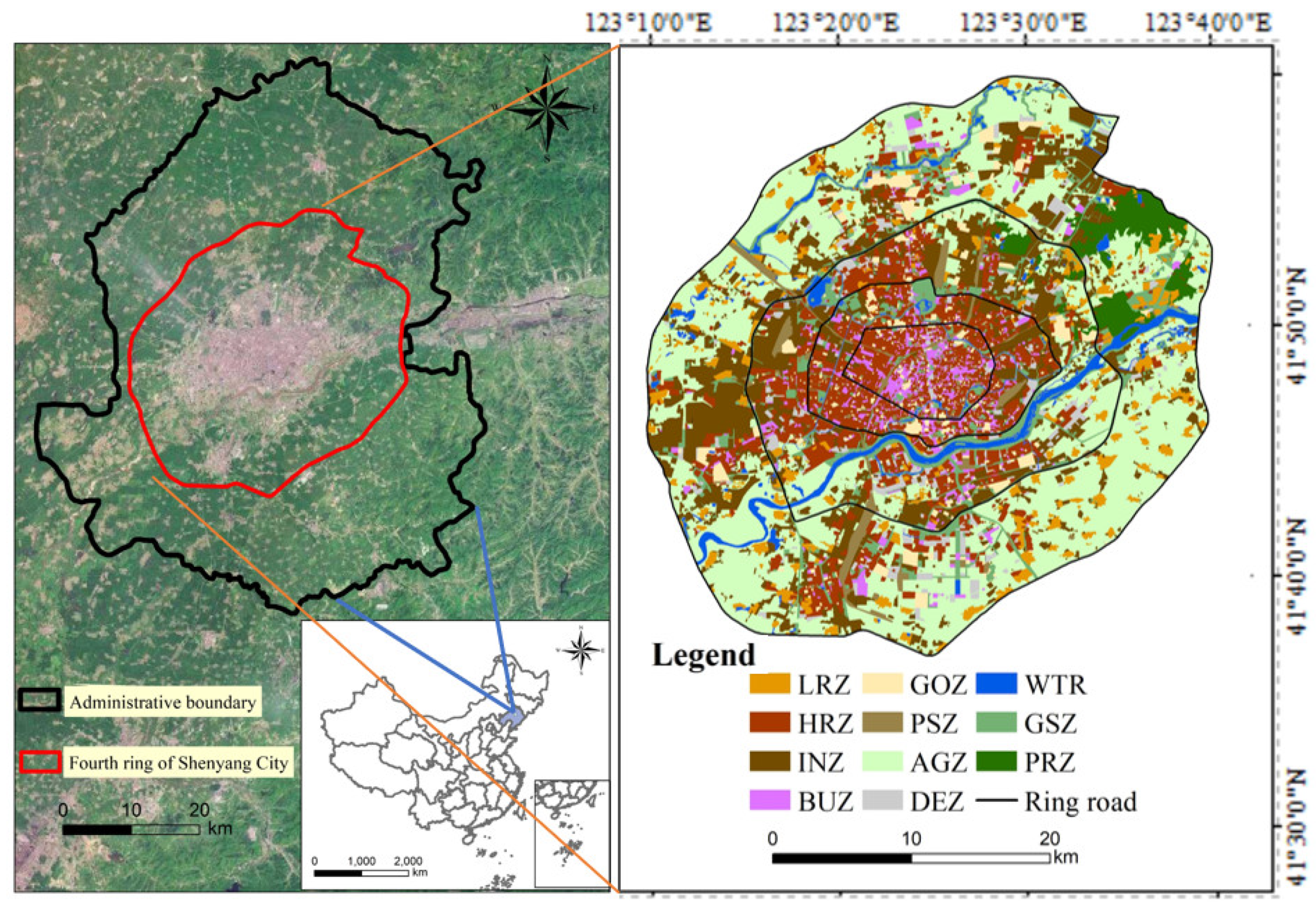
2.1. Study Area and Data

Shenyang (41°09′ N–41°55′ N, 123°16′ E–123°36′ E) is located in the southern part of Northeast China, comprises an area of 12,600 km², and is the economic, cultural, and commercial center of the Northeast region (Figure 1). The fourth ring area contains the built-up area, which covers 1235.25 km² and has a high population density and complicated surface types.

Using OpenStreetMap (https://www.openstreetmap.org/, accessed on 2 May 2020) to obtain the road data, the whole region was divided into blocks based on the main boundaries. Referring to the definitions of UFZs by other researchers [40,41], the final functional area was divided into 11 types and combined with the Baidu map (

Table 1. Classification and characteristics of urban functional zones (UFZs) in the Shenyang fourth ring area [40].

UFZ	Code	Description
Low-density residential zone	LRZ	Typical residential communities, with sparse populations and low buildings.
High-density residential zone	HRZ	Typical residential communities, including multiple-family houses and apartments with dense populations.
Industrial zone	INZ	Factories for manufacturing, repair stations, and storage land.
Business zone	BUZ	Offices for finance organizations and markets, restaurants, and hotels.
Government zone	GOZ	Governments, public organizations, schools, colleges, and institutes.
Public service zone	PSZ	Public service areas, such as stadiums, libraries, museums, and hospitals.
Agricultural zone	AGZ	Cultivated land, greenhouses, and other agricultural facilities.
Development zone	DEZ	Undeveloped open spaces and construction sites.
Green space zone	GSZ	Urban parks and scenic zones with high green coverage.
Water	WTR	Open water, including rivers, reservoirs, ponds, and ditches.
Preservation zone	PRZ	Open space with natural and artificial green space, such as forest parks.

).

LST was retrieved using Landsat8 images. Landsat8 is equipped with the Operational Land Imager (OLI) and the Thermal Infrared Sensor (TIRS). The OLI has nine bands, including a panchromatic band with a spatial resolution of 15 m and the rest with a 30 m resolution [42]. TIRS also includes two separate thermal infrared bands to facilitate more accurate LST [43]. To minimize the cloud effect, the cloud coverage of images selected in the study was less than 10%.

We used Barista software [44] to extract the outline and height of buildings using visual interpretation with Google images (1 m) from 2020. Field surveys were used for accuracy verification. Buildings were divided into six categories by height: single-story buildings (height ≤ 5 m, SSB), low-rise buildings (5 m < height ≤ 10 m, LSB), multistory buildings (10 m < height ≤ 24 m, MSB), mid-rise buildings (24 m < height ≤ 50 m, MRB), high-rise buildings (50 m < height ≤ 100 m, HRB), and superhigh-rise buildings (height > 100 m, SHRB).

2.2. Method

The spatial pattern and relative influence of factors of the UNHI/UNCI effect were analyzed in this paper to reflect the status of the urban thermal environment. The LST was retrieved using the radiative transfer equation, and the mean standard deviation was used to divide urban thermal landscapes into five grades. Using the sky view factor (SVF) to describe the spatial characteristics of buildings and explore the relationships between 3D buildings and the neighborhood thermal environment. Focal Statistics was used for neighborhood analysis of the LST data. The impacts of green space patches on UNHI and UNCI were examined using buffer analysis. Finally, the analysis of the relative contribution of factors affecting the UNHI and UNCI effects was conducted using the boosted regression trees (BRT).

2.2.1. Urban Thermal Landscapes Analysis

The radiative transfer equation was used to retrieve the LST [45,46], where $L_T$ is the surface-leaving radiance, $L_{\lambda }$ indicates the value of infrared thermal radiation, $\epsilon$ is the land surface emissivity, $L_{\mathsf{\mu }}^{\uparrow }$ is the atmospheric upward radiation, $L_d^{\downarrow }$ is the atmospheric downward radiance, $\tau$ is the atmospheric transmissivity, $T_B$ is the effective brightness temperature, $K_1$ (774.89 W/(m² sr mm)) and $K_2$ (1321.08 K) are the calibration parameters of the infrared band, $\lambda$ refers to the wavelength of emitted radiance (10.9 µm), and $\rho$ = 1.438 × ${10}^{-2}$ mK.

$$L_T=\frac{L_{\lambda }-L_{\mathsf{\mu }}^{\uparrow }-\tau \cdot \left(1-\epsilon \right)\cdot L_d^{\downarrow }}{\epsilon \cdot \tau }$$

(1)

$$T_B=\frac{K_2}{ln\left(\frac{K_1}{B\left(T_S\right)}+1\right)}$$

(2)

$$\mathrm{LST}=\frac{T_B}{1+\frac{\lambda T_B}{\rho }\ln \epsilon }$$

(3)

The mean standard deviation was used to classify urban thermal landscapes and reveal the evolution of the spatial pattern characteristics of urban surface thermal landscapes [47]. The LST was divided into five thermal landscape grades (

Table 2. The classification criteria of the land surface temperature (LST).

Temperature Zone (TZ)	Temperature Range
Low-temperature zone (LTZ)	$T_{ni}$<$T_{mean}$ − 1.5 S
Sub-low-temperature zone (SLTZ)	$T_{mean}$ − 1.5 S ≤ $T_{ni}<T_{mean}$ − 0.5 S
Medium-temperature zone (MTZ)	$T_{mean}$ − 0.5 S ≤ $T_{ni}<T_{mean}$ + 0.5 S
Sub-high-temperature zone (SHTZ)	$T_{mean}$ + 0.5 S ≤ $T_{ni}<T_{mean}$ + 1.5 S
High-temperature zone (HTZ)	$T_{ni}$ ≥ $T_{mean}$ + 1.5 S

Note: $T_{ni}$ is the real temperature of surface pixels, $T_{mean}$ is the average temperature of all surface pixels, and S is the standard deviation.

).

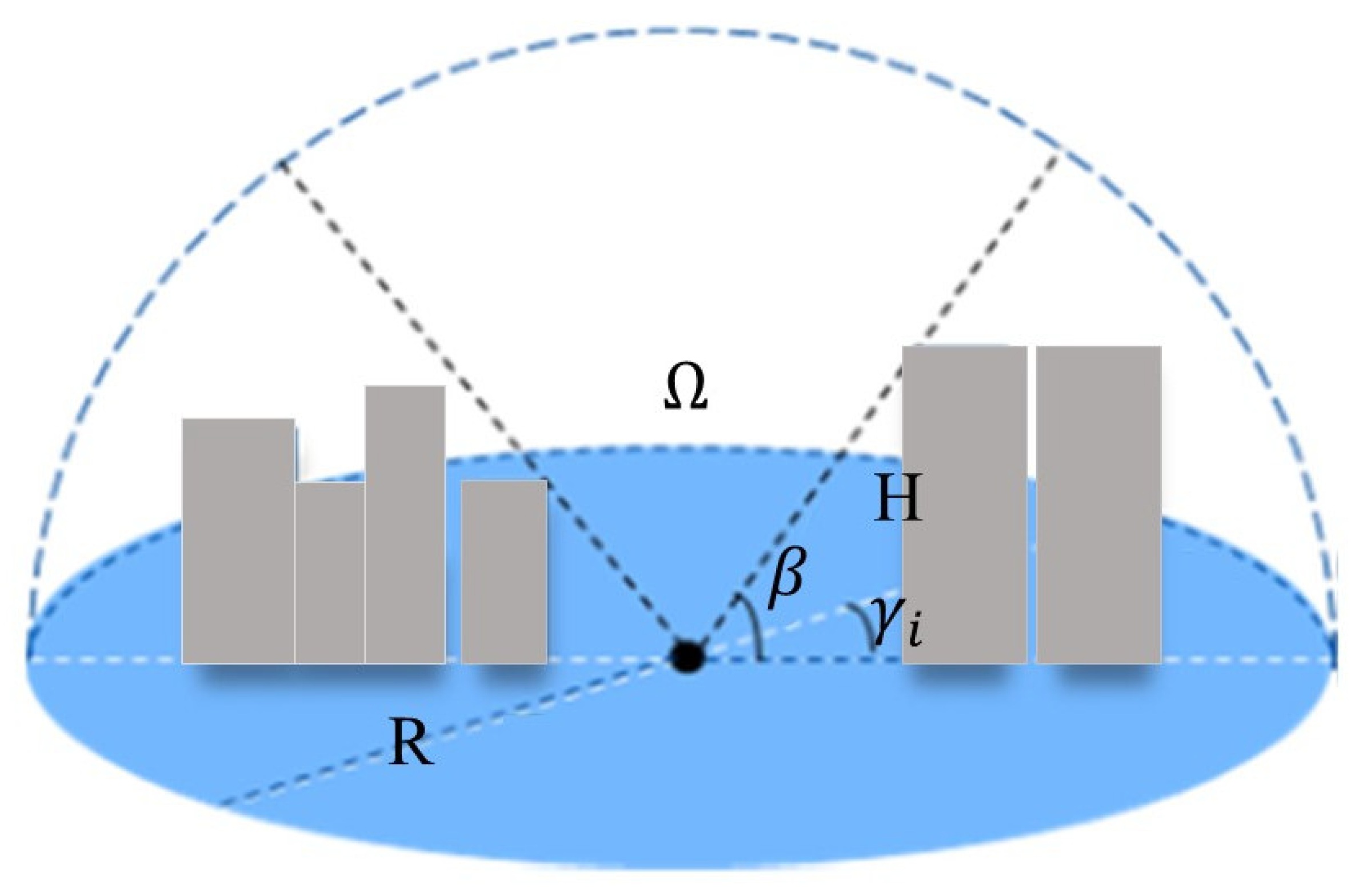
2.2.2. Sky View Factor

SVF is the ratio of the visible sky extent in the open space enclosed by a building and it is a common parameter used to describe the spatial characteristics of buildings (Figure 2) [48]. The SVF is one of the important factors affecting the UHI, and scholars have studied the correlation between the SVF and the thermal environment [49,50]. The value of SVF ranges from 0 to 1, with 0 indicating that the upward space of the observation point is completely shaded and 1 indicating that it is completely open and unshaded. Our study explored the relationships between the SVF of buildings and the UNHI/UNCI.

As shown in Equation [51],

$$SVF=1-\frac{{{\displaystyle \sum }}_{i=1}^{n}sin{\gamma }_i}{n}$$

(4)

$${\gamma }_i=\mathrm{arc}\tan \frac{H}{R}$$

(5)

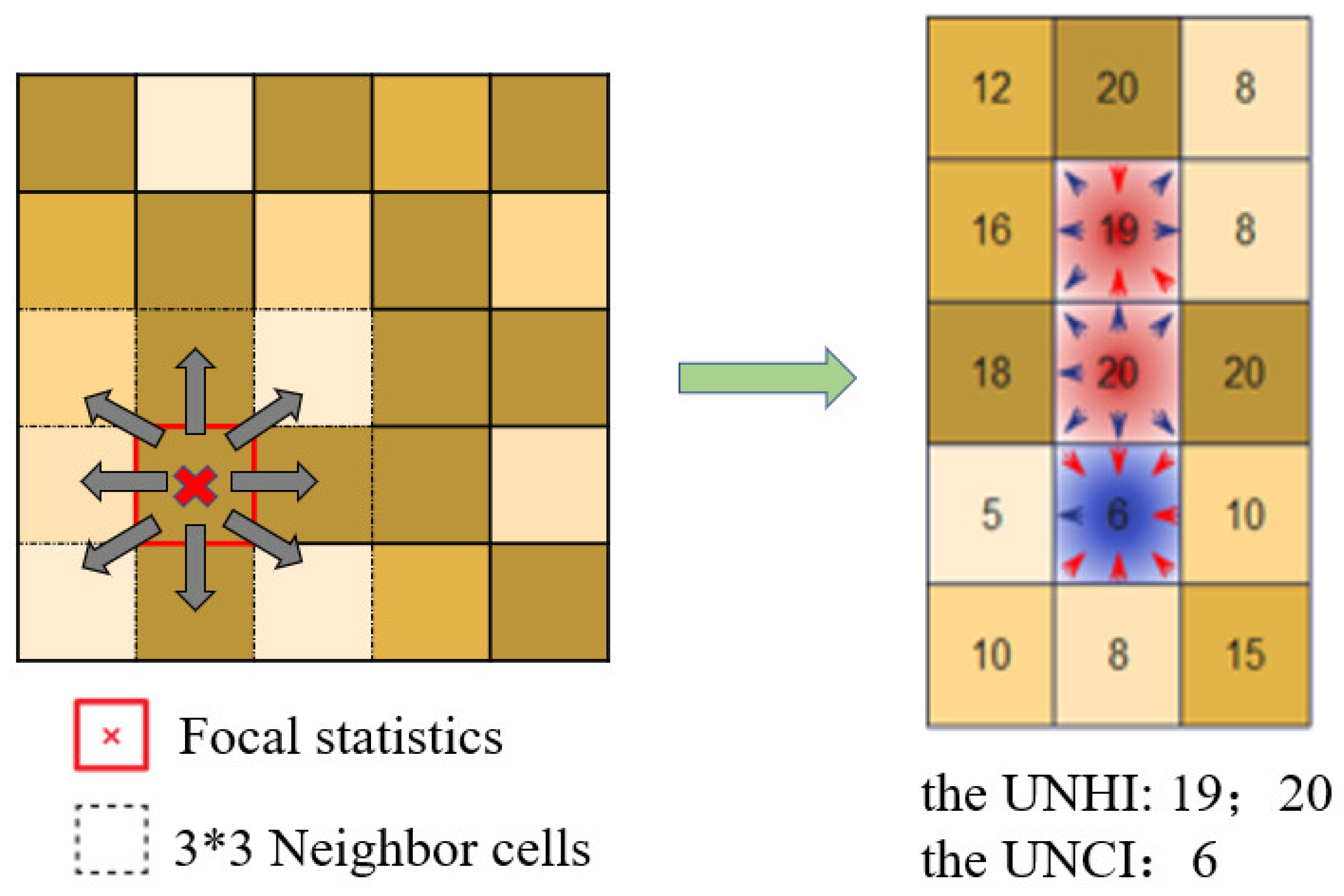
2.2.3. Spatial Neighboring Analysis

The local climate velocity is a vector that describes the speed and direction at which points on a grid map need to move in order to remain stationary in a climate space under climate change [52]. The estimation of the spatial gradient of the climate depends on the neighboring cells [53,54]. When calculating a geographical unit’s local climate velocity, the variable’s corresponding spatial gradient is required. Based on the local climate velocity, a neighborhood analysis of the LST data in 2020 was performed. The calculations were performed in ArcGIS using Focal Statistics. Through accessing each pixel in the raster, the average value of all input pixels was output in a specified neighborhood range (a square of three pixels in both height and width; Figure 3).

We can calculate Δi as the difference between the mean value of LST ($LS{T}_{mean}$) and its neighboring cell value. If Δi is greater than 0, it is the UNHI. If Δi is less than 0, it is the UNCI.

$$\mathsf{\Delta }\mathrm{i}=LS{T}_i-LS{T}_{mean}$$

(6)

The vector field raster function U-V was used to describe residents’ perceptions of the UNHI and UNCI effects. To obtain the speed and direction of the wind, weather stations use anemometers to measure the wind speed in two mutually perpendicular directions, U and V, where U is the latitudinal velocity, and V is the longitudinal velocity. The vector field raster function in ArcGIS was used to synthesize and convert the raster into a U-V dual-band. The conversion formula was as follows:

$$\mathrm{u}=\mathrm{m}\times \cos \left(\mathsf{\pi }\times \mathrm{d}/180\right)$$

(7)

$$\mathrm{v}=\mathrm{m}\times \sin \left(\mathsf{\pi }\times \mathrm{d}/180\right)$$

(8)

$$\mathrm{m}=\mathrm{sqrt}\left(\mathrm{u}\times \mathrm{u}+\mathrm{v}\times \mathrm{v}\right)$$

(9)

$$\mathrm{d}=\mathrm{atan}2\left(\mathrm{v}/\mathrm{u}\right)\times 180/\mathsf{\pi }$$

(10)

where u is the vector U, is the vector V, m is the magnitude, and d is the direction (°).

2.2.4. Buffer Analysis

To analyze the influence of green space patches on the cooling effect, they were classified into five grades (

Table 3. Green patch grades.

Patch Grades	Patch Areas (hm2)	Patch Characteristics
1	S ≤ 1	Tiny patch (TP)
2	1 < S ≤ 5	Small patch (SP)
3	5 < S ≤ 10	Medium patch (MP)
4	10 < S ≤ 20	Large patch (LP)
5	S > 20	Super large patch (SLP)

) [20,55].

Buffer analysis was used to analyze the UNHI and UNCI effects of green space patches. First, 20 annular buffer zones were established around the green patch, and the buffer interval was set to 100 m. Then, the mean LST of each ring buffer was set as the dependent variable, and the buffer interval was set as the independent variable. The distance decay model was used for fitting [56]:

$$\mathrm{y}=\mathrm{a}+\mathrm{b}\times r^D$$

(11)

where a denotes the maximum value of LST within the buffer, b denotes the difference in LST between the interior and exterior of the green space patch, r represents the attenuation coefficient, and D is the distance from the green space patch (m).

In addition, the cooling effect of urban green space on neighboring areas decayed with increasing distance [12,57]. Regression analysis was used to further evaluate the distance of the cooling effect. The influence distance was defined as the distance corresponding to the attenuation of the cooling amplitude to 10%. The impact distance was calculated as

$$L_i=\ln 0.1/\ln r$$

(12)

where $L_i$ is the influence distance of the cooling effect (m).

2.2.5. Boosted Regression Trees

The BRT was chosen to analyze the relative influence of factors affecting the UNHI and UNCI effects. Based on the traditional classification regression tree algorithm, BRT generates multiple regression trees through randomly selecting and autonomously learning from the tree model to optimize the prediction performance and improve the prediction accuracy of the model, which is an effective method for assessing relevant independent variables and solving classification as well as prediction problems [58,59]. This study used UNHI and UNCI effects as the response variable. A total of 11 UFZs were selected as independent variables using R software 4.1.3, with “dismo” and “gbm” packages. The learning rate was 0.005, and the bag fraction was 0.5.

3. Results

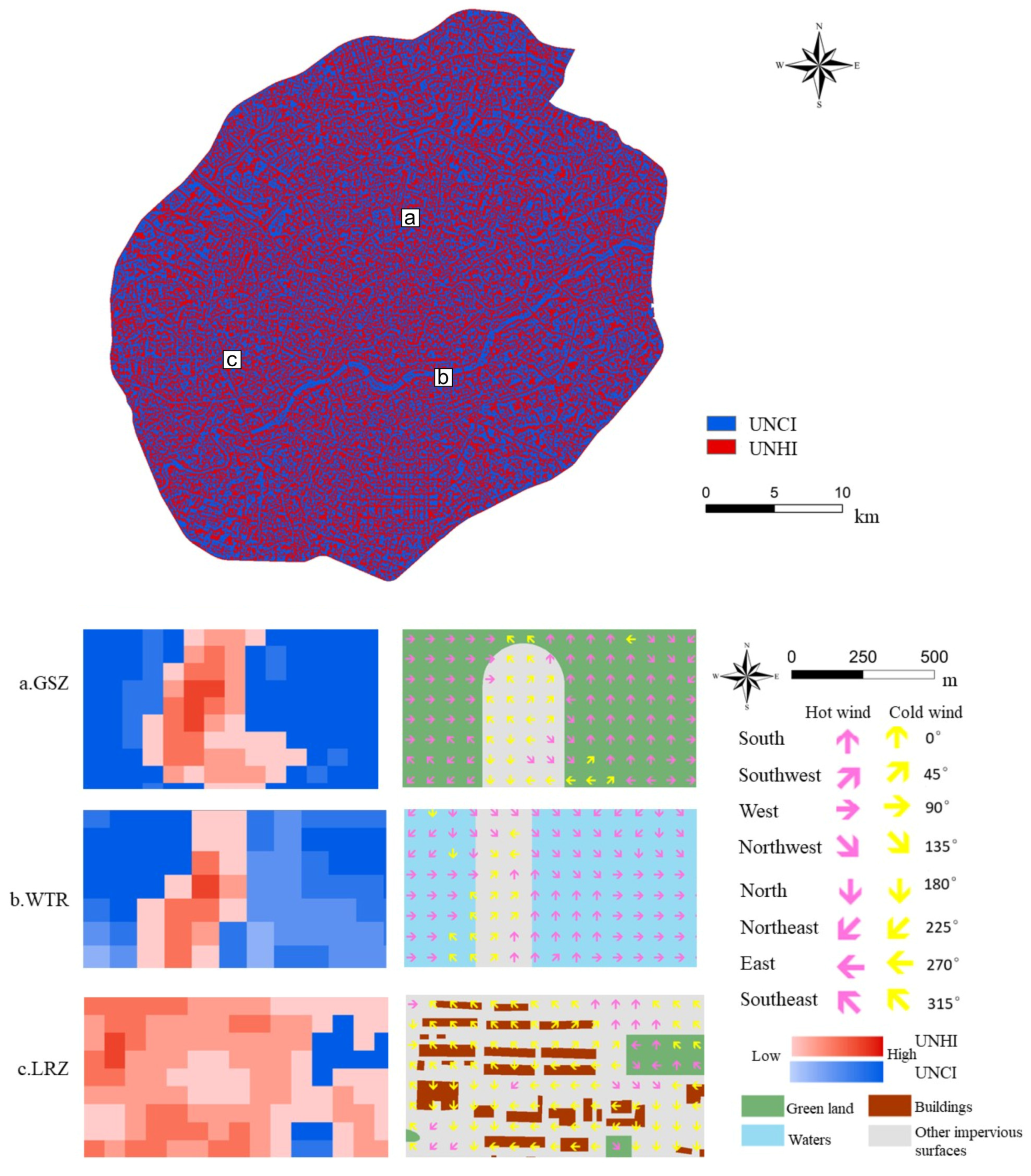
3.1. Distribution of the UNHI and UNCI

The distribution of the UNHI/UNHI and the wind direction within the fourth ring area of Shenyang City was as follows (Figure 4). There was a “hot wind” from the UNHI and a “cold wind” from the UNCI, both with eight directions. In summer, residents were more likely to feel the “cold wind.” Figure 4a was mainly part of the UNCI, while other impervious surfaces were the UNHI. The square in the Qingnian park divided the large green patches originally connected in the middle, which mitigated the UNCI effect of the GSZ. The center of the square had a relatively higher UNHI effect, and the effect decreased from the center to the periphery. The edge of the GSZ near the square had a lower UNCI effect. The WTR in Figure 4b reflected an obvious UNCI effect. However, the Nanyang Lake Bridge running through the middle of the Hun River changed the morphology of the water patches, diminished the convective heat transfer radiation, and weakened the cooling effect of the WTR. The buildings constituted the LRZ in the middle of Figure 4c. Green land distributed inside the LRZ produced the UNCI effect, which also weakened the UNHI effect of the LRZ near its edge. Our results identified the UNHI/UHCI in the large piece of UCI/UHI more finely.

3.2. Relationships between 3D Buildings and the Neighborhood Thermal Environment

3.2.1. Relationships between Building Classification and the UNHI/UNCI

The proportions of building classification in the UNHI and UNCI were counted (Figure 5). The proportions of the MRB, HRB, and SHRB in the UNCI were higher than those in the UNHI, while the SSB, LSB, and MRB were the opposite. Among them, MSB accounted for the largest proportion, which was the main building type in the city. With the increase in building height, the difference between UNHI and UNCI of SSB, LRB, and MSB gradually increased. The difference between UNCI and UNHI of MRB, HRB, and SHRB decreased. Within a certain range, the neighborhood LST had a significant lowering effect as the building height increased.

3.2.2. Relationships between the SVF and the UNHI/UNCI

The correlation between the SVF and UNHI/UNCI was analyzed using linear fitting, and the fitted function was y = 0.09x − 0.02, R² = 0.69 (Figure 6). According to the fitting results, the effect of UNCI was weakened but the effect of UNHI was enhanced with the increase in SVF. The area with lower SVF often distributed higher buildings in the narrower streets. Higher structures intensified the degree of shielding from solar radiation and formed a larger range of shadow areas, which resulted in a stronger UNCI effect. As the area became increasingly wide-open, the surface with low heating capacity that directly received more solar radiation warmed up rapidly, so the UNHI effect was enhanced significantly.

3.3. Relationships between Green Patches and the Neighborhood Thermal Environment

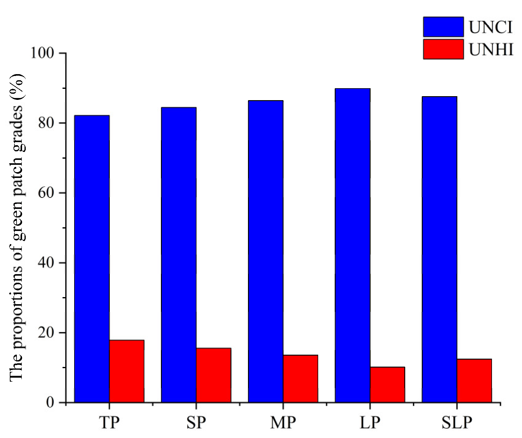
3.3.1. Relationships between Green Patch Grades and the UNHI/UNCI

A total of 85.17% of the GSZ were located on the UNCI, and 14.83% were located on the UNHI, indicating that the distribution of GSZ played an important role in the reduction of neighborhood LST.

Figure 7 showed the proportions of different green patch grades in the UNHI and the UNCI. With the increase in the green space patch area, the proportions of the UNCI increased gradually. The proportions of the UNCI of TP, SP, MP, and LP were 82.16%, 84.45%, 86.43%, and 89.88%, respectively. The percentage of SLP was 87.54%, which was slightly lower than that of LP but higher than MP.

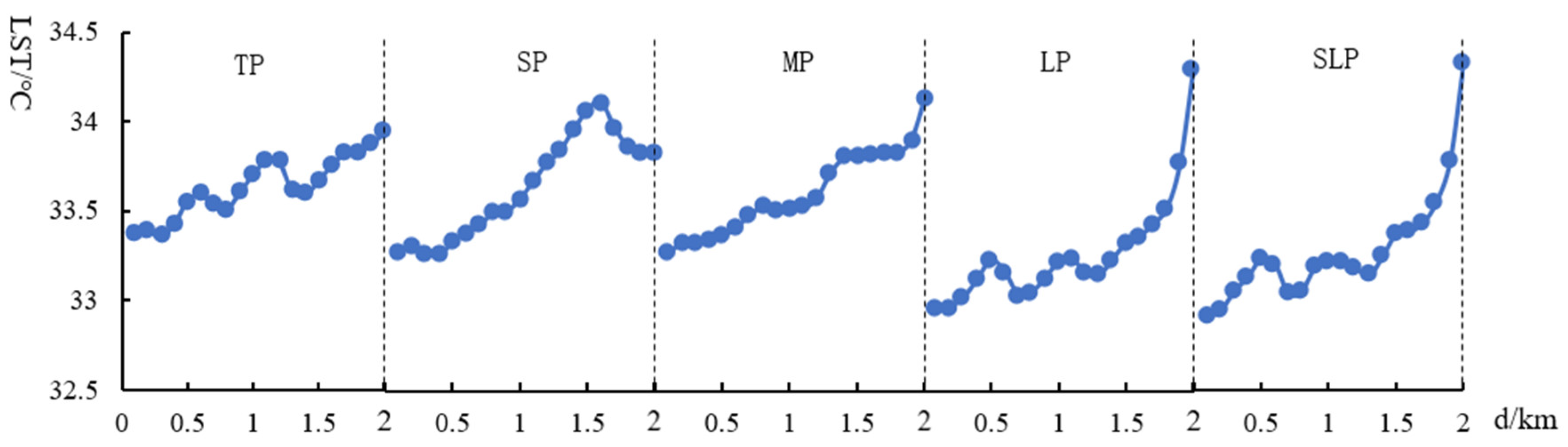
3.3.2. Cooling Effect of Green Patch Grades

With the increase in the green patch area, its cooling effect was gradually enhanced (Figure 8). However, whether the patch area was large or small, this cooling effect decreased with the increase in the buffer distance. Within a 2 km buffer distance, the maximum difference in the temperature drop amplitude of TP, SP, MP, large patches, and SLP was 0.55 °C, 0.56 °C, 0.86 °C, 1.34 °C, and 1.42 °C, respectively. Green patches not only had a significant cooling effect on the interior but also a more obvious cooling effect on the surrounding environment. The fitting results of the distance decay model (

Table 4. Analysis of cooling amplitude of green patch grades.

Patch Characteristics	a/°C	b/°C	r	Li/km
TP	47.47 ± 0.34	−0.33 ± 0.04	0.03 ± 0.01	0.66
SP	47.15 ± 0.38	−0.75 ± 0.06	0.11 ± 0.01	1.09
MP	46.62 ± 0.35	−1.04 ± 0.05	0.15 ± 0.01	1.21
LP	46.76 ± 0.31	−2.14 ± 0.07	0.32 ± 0.01	2.08
SLP	46.77 ± 0.29	−3.45 ± 0.07	0.36 ± 0.01	2.25

Note: TP: tiny patch; SP: small patch; MP: medium patch; LP: large patch; SLP: super large patch.

) showed that with the increase in the patch area, the greater the cooling amplitude, the greater the influence distance. The cooling ranges of the MP, LP, and SLP were greater than 1 °C. The SLP was the largest, reaching 3.45 °C. The cooling distances of the SP, MP, LP, and SLP were more than 1 km. The SLP was the largest, reaching 2.25 km.

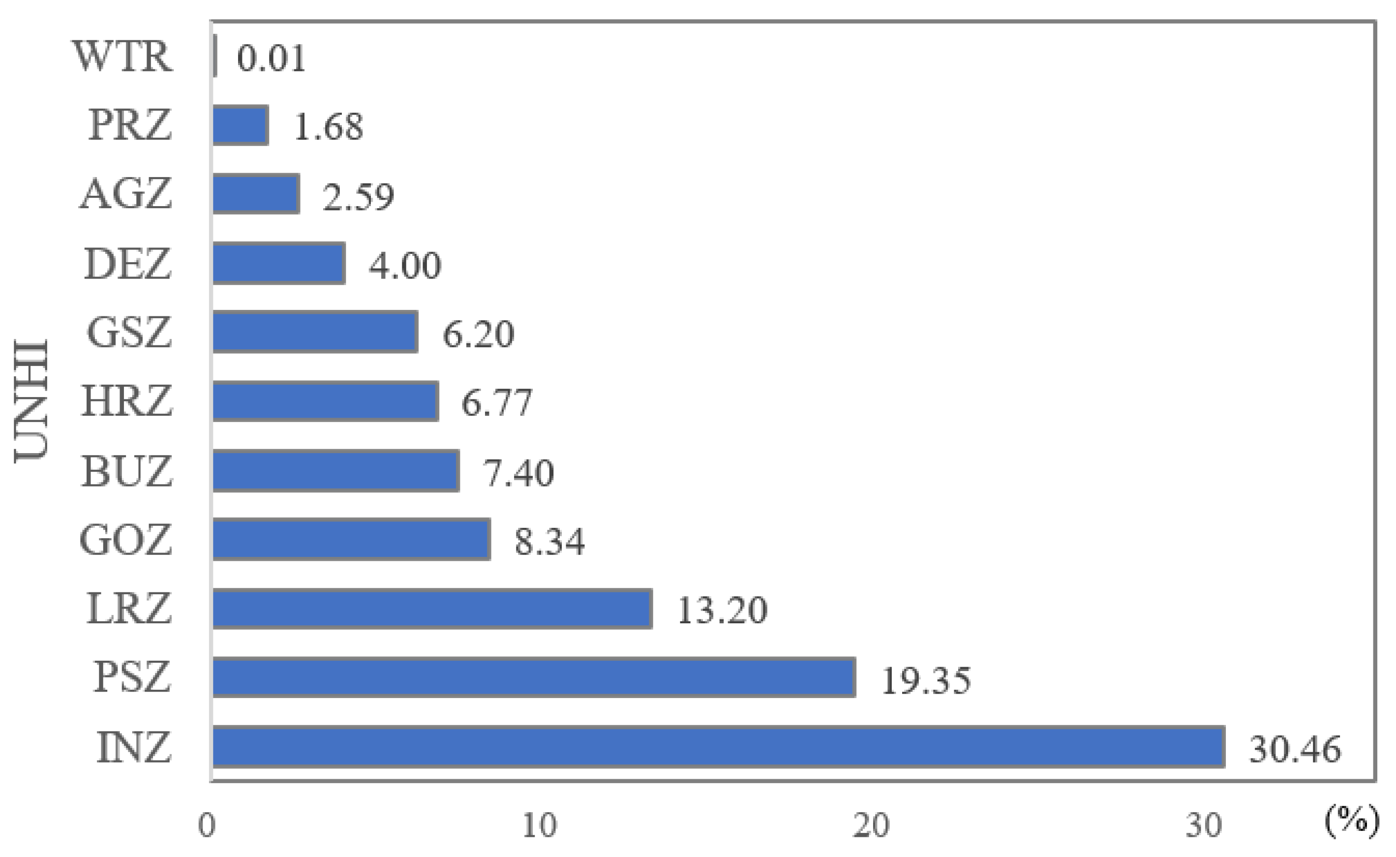
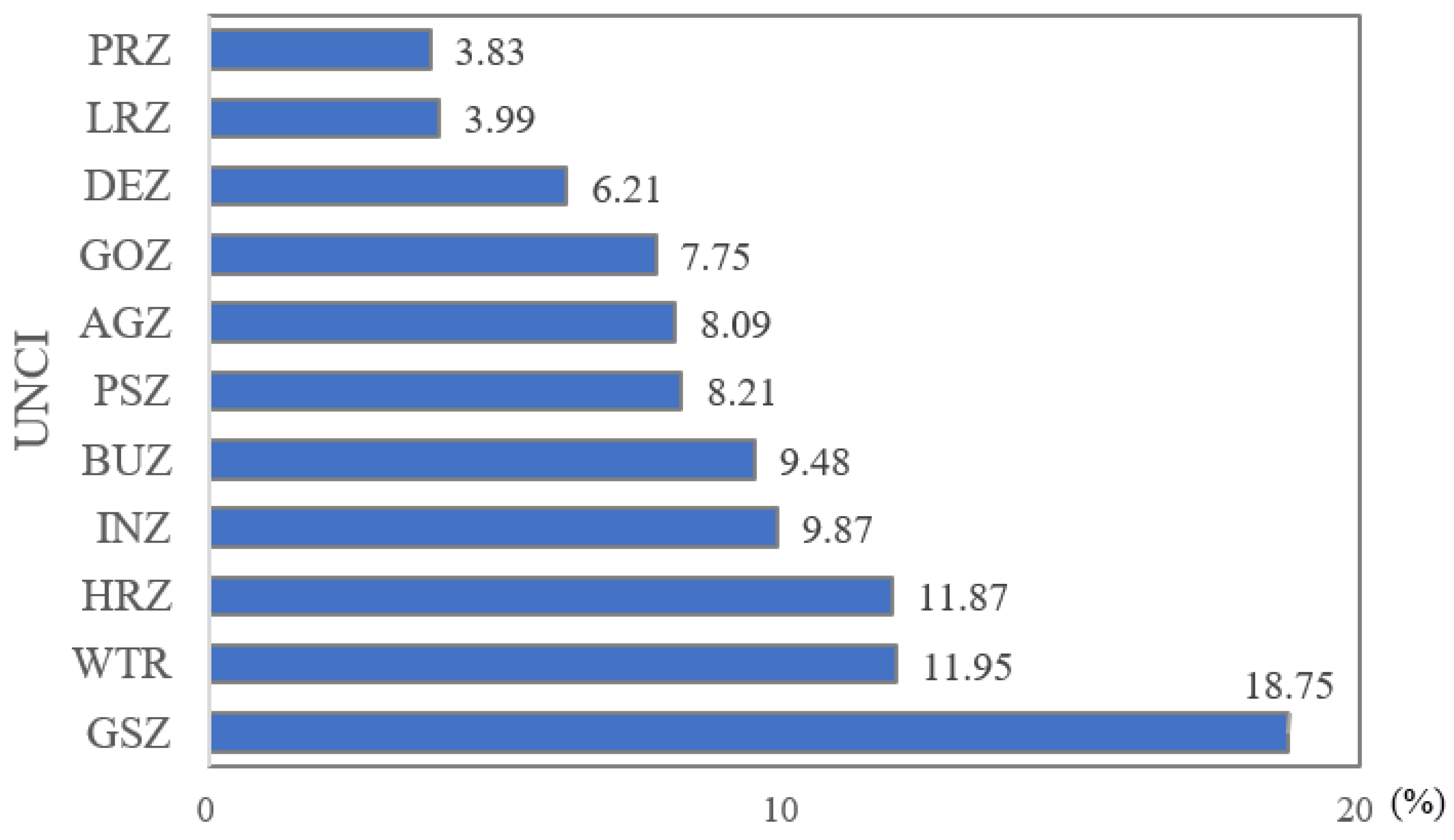
3.4. Relationships between the UFZs and the Neighborhood Thermal Environment

3.4.1. Relationships between the UFZs and the Urban Thermal Landscapes

According to the distribution of TZs in the UFZs (

Table 5. The proportions of land surface temperature (LST) grades in the urban functional zones (UFZs). HTZ: high-temperature zone; SHTZ: sub-high-temperature zone; MTZ: medi-um-temperature zone; SLTZ: sub-low-temperature zone; LTZ: low-temperature zone. WTR: water; PSZ: public service zone; PRZ: preservation zone; INZ: industrial zone; LRZ: low-density residential zone; HRZ: high-density residential zone; GSZ: green space zone; GOZ: government zone; DEZ: development zone; BUZ: business zone; AGZ: agricultural zone.

Proportions (%)	LTZ	SLTZ	MTZ	SHTZ	HTZ
AGZ	-	39.58	41.13	17.77	1.52
BUZ	-	-	3.09	39.62	57.29
DEZ	-	2.03	17.45	66.03	14.49
GOZ	-	-	8.23	58.01	33.76
GSZ	-	9.06	50.48	37.79	2.66
HRZ	-	-	12.67	60.28	27.05
LRZ	-	0.15	17.15	59.30	23.41
INZ	0.69	1.78	6.62	37.72	53.18
PRZ	-	-	54.77	43.85	1.37
PSZ	-	-	7.32	37.62	55.06
WTR	1.48	52.56	32.89	11.28	1.79

), the INZ was dominated by the HTZ (45.64%), and the HRZ was dominated by the SHZ (25.30%). The AGZ occupied the highest proportion in both the MTZ (54.64%) and SLTZ (75.28%), while the INZ and WTR occupied the highest proportion in the LTZ (71.78%). The other UFZs were the WTR (28.22%). This might be because the total area of the INZ was relatively large, about five times greater than the area of the WTR, so the area’s proportion was also relatively large. This part of the INZ was mostly smaller, with less industrial heat rejection, which had little impact on the overall temperature. The BUZ had the highest LST (40.02 °C), 57.29% of which was located in the HTZ, and the area of the HTZ and UHTZ accounted for 96.91% of the total area of the BUZ. Regarding spatial distribution (Figure 9), the BUZ was concentrated within the first and the second ring, where human activities were relatively intensive and produced high anthropogenic heat emissions, promoting the increase in the LST. The LST of the INZ was 39.95 °C, 53.18% of which was located in the HTZ, and the area of the HTZ and UHTZ accounted for 90.91% of the total area of the BUZ. The INZ was mainly located in the third and fourth rings, accounting for 60.47% and 31.40% of the total area, respectively. Only 8.13% of INZs was sporadically distributed within the first and the second ring. Larger INZs were mainly located in the western and northern parts of the fourth ring. The LST of HRZ and LRZ were 38.92 °C and 38.91 °C, respectively. The HRZ was concentrated in the first, second, and third ring, accounting for 73.33%. Meanwhile, the LRZ was concentrated within the fourth ring, accounting for 82.35% of its total area. The LSTs of GOZ and PSZ were lower than that of residential zones. The spatial pattern of their buildings was more scattered, which collected less heat internally and was difficult to transfer continuously, so the heating effect was more limited. The LST of DEZ was lower than that of the PSZ but significantly higher than that of the GSZ. The distribution within the third and fourth rings accounted for 87.80%. Especially within the fourth ring, the DEZ was mostly surrounded by the AGZ, which also had a certain cooling effect. The LST of the GSZ was only 35.97 °C, which was significantly lower than that of the preceding UFZs. The GSZ only accounted for 3.63% of the area of the first ring in the city center, mainly Wanquan Park, Zhongshan Park, Bitang Park, and other urban parks. The LST of WTR was lower than that of the AGZ, which was 33.44 °C. Among them, the SLTZ accounted for more than half, about 52.56%. The WTR had a high specific heat capacity, and its evaporation and convection processes could play a cooling role. The PRZ, mostly forest parks and nature reserves, had the lowest LST (32.24 °C). The SLTZ accounted for 54.77% of its total area. The PRZs were mainly located in the third and fourth ring areas, with an area ratio of 71.55%. PRZ accounted for a large proportion of the urban vegetation cover area and showed a significant negative correlation with increased LST.

3.4.2. Relative Influence of UFZs on the UNHI/UNCI

The effects of UFZ classification on the UNHI/UNCI were complex, and the study of multi-factor interaction was the key to further understanding the mechanism of the urban thermal environment. The results showed that the relative importance of different UFZ classifications varied in the UNHI and the UNCI. For the UNHI (Figure 10), the INZ was the largest influencing factor (30.46%), followed by the PSZ (19.35%), and the combined contribution of the two factors was nearly half of the total contributions. The influencing factors included the LRZ (13.20%), GOZ (8.34%), BUZ (7.40%), HRZ (6.77%), and DEZ (4.00%). The smallest contributions were made by the AGZ (2.59%) and PRZ (1.68%). For the UNCI (Figure 11), the GSZ had the highest impact (18.75%), followed by the WTR (11.95%), HRZ (11.87%), and INZ (9.87%), respectively. The contribution rate of the top four factors exceeded 50% of the total rate. The next most influential factors were the BUZ (9.48%), PSZ (8.20%), AGZ (8.09%), GOZ (7.75%), DEZ (6.21%), LRZ (3.99%), and PRZ (3.83%). In general, there was a small difference in the contribution of the factors influencing the UNCI.

4. Discussion

4.1. Improvement in the Neighborhood Thermal Environment

The spatial patterns of the neighborhood affect its thermal environment. Adding green space in residential areas can alleviate the thermal environment in the neighborhood in summer. The reasonable dispersion of green patches can also weaken the spatial diffusion effect of impervious surfaces such as construction land and better play a cooling effect. For example, as shown in Figure 4c, urban green corridors can block heat advection from neighboring landscapes, and urban green belts can divide residential areas into different zones which, to a certain extent, impede the transfer of high-temperature heat to the surrounding areas. Previous studies have also shown the same results [60,61]. At a specific research scale, the cooling effect of water in the same area is even better than that of green spaces, which was also proved in Wuhan City [62]. However, due to the needs of urban construction, such as the construction of bridges and other anthropogenic factors, like Figure 4b, the relatively stable natural environmental matrix of large water bodies is destroyed, reducing the connectivity of the watersheds and destroying the thermal environmental regulation benefits of the water bodies overall [63]. Therefore, transforming natural waters to other land uses, such as construction lands, should be restricted. In the previous studies of Shenyang, Hun River was regarded as the UCI [64,65]. Our research explored a new approach to identify the distribution of UNHI within a large area of UCI on a finer scale, as well as the distribution of UNCI within the large patches of UHI. In cities with limited construction lands, breaking the dense building layout and rationally matching low-density and high-density residential zones can also support temperature regulation, thus alleviating the local thermal environment.

4.2. Influence of 3D Buildings on the UNHI and UNCI Distribution

With an increase in building height, the degree of solar radiation shading is enhanced, which reduces the LST to a certain extent. Therefore, in planning urban residential areas, the thermal environment can be improved by appropriately increasing building height [66]. In summer, in very low SVF areas such as narrow streets and deep canyons surrounded by high-rise buildings, building shadows block solar radiation and form a larger range of shadow areas. The shadow areas form a temperature difference and generate heat exchange with impervious surfaces exposed to solar radiation, furthering the UNCI, which was also confirmed in other studies [50,67]. When the SVF increases gradually, the difference decreases, and the effect of LST reduction is relatively weak. The heat is absorbed due to impervious surfaces such as asphalt and concrete that receive solar radiation. At the same time, the heat is also transferred to the surrounding environment, resulting in a significant increase in the temperature of the near-surface layer, making the LST continue to be higher than that of the neighboring environment. In addition, with the increase in the SVF, more green space may be considered. Although the shading effect of vegetation can reduce the LST, relevant research showed that compared with architectural shading, vegetation shading is less intensive [68,69]. Therefore, relative to the region with high SVF, the UNHI effect is still increasing.

4.3. Factors Influencing the UNHI and UNCI

The BUZ is mostly located in the urban center, with a relatively high level of urbanization. Over-dense building distribution and excessive building attributes reduce the rate of air circulation and heat exchange, leading to an excessively high LST. For the INZ, a large amount of fuels, such as coal, oil, and natural gas, is used in the industrial production process. The fuel consumption process is accompanied by heat release into the atmosphere. With the acceleration of urbanization, residential zones have become the basic unit for many research studies on urban internal structures and environments [70]. Residential areas usually have a high proportion of building units with building materials with low specific heat capacities, which will heat up rapidly under summer insolation and increase the LST of the neighboring environment. The results have been replicated in studies in other cities, like Minneapolis and Lagos [71,72]. In addition, the buildings distributed along the street form a canyon effect, which inhibits the radiation of heat and ultimate absorption by impervious surfaces [73]. Compared to the HRZ, the LRZ has less building density and better air circulation; thus, the warming effect is relatively limited [74]. There are more natural surfaces surrounding the LRZ, such as green spaces and water, which have relatively high albedo, helping to form the UNCI. In urban planning, street trees, green roofs, and artificial grasslands have been used as effective environmental configurations to mitigate the UHI effect [75,76]. As the “blue space” of the city, water bodies such as rivers, reservoirs, and lakes can produce the UNCI effect. Some studies have conducted quantitative analyses on the cooling effect of typical city water bodies. For example, the Huangpu River, the largest river in Shanghai, has a cooling intensity of 4.2–9.1 °C compared to the surrounding environment [77,78].

In the UNHI analysis of the contribution of UFZs, the LST of PSZ is not higher than that of other UFZs. This is mainly because, although its total area share is relatively small (2.5%), the HTZ accounts for 55.06% of the urban thermal landscape. For residential zones, although the total proportion and LST of the LRZ are higher than the HRZ, its contribution value is relatively high. This may be because although LRZs are more numerous, the single area is smaller. Smaller patches are more susceptible to interference by the neighborhood environment. Previous studies have shown that the internal core zones are much smaller than the edge zones, leading to instability in the internal environment [79,80]. The GSZ and WTR UFZs have the largest contribution, which coincided with the results of the cooling effect of urban blue-green space obtained from previous studies [81,82]. The cooling effect generated by urban spaces such as rivers, reservoirs, and lakes not only affects themselves but also has a certain impact on the surrounding environment. The HRZ has a high degree of UNHI effect, which may be because the dense building distribution blocks solar radiation and generates more shadow areas, which enhances the reduction in the LST.

4.4. Limitations and Future Avenues

Our study provided a new way to improve the urban thermal environment and enhance the livability of human settlements. However, there were some shortcomings. Studies have shown that anthropogenic heat emission had a stronger impact on LST change in winter than in summer [83]. In future studies, further analysis of the UNHI effect in different seasons can be carried out. In addition, the urban thermal environment was also affected by weather conditions such as precipitation and wind speed. In the future, the atmospheric boundary layer temperature, humidity, and wind speed under the urban canopy structure can be analyzed in combination with the weather conditions, to make the research on the UNHI and its influencing factors more comprehensive.

5. Conclusions

This study explored the UNHI and UNCI effects based on RS data to investigate how the LST of the localized area was affected by the spatial type and morphology of neighboring areas from the perspective of urban 3D buildings, urban green space, and UFZs. The relationships between 3D buildings and the neighborhood thermal environment indicated that higher buildings enhanced the degree of solar radiation shading, which exhibited an obvious lowering effect on the neighborhood LST. Then the UNHI effect was enhanced with the increase in the SVF. The distribution of green space played an important role in lowering the LST of the neighborhood, and the cooling effect of different green patches differed. With an increase in the area of the patch, its cooling range and influence distance increased gradually. The INZ had the greatest impact on the UNHI effect, followed by the PSZ, LRZ, GOZ, BUZ, HRZ, GSZ, DEZ, AGZ, PRZ, and WTR. The GSZ had the greatest influence on the UNCI effect, followed by the WTR, HRZ, INZ, BUZ, PSZ, AGZ, GOZ, DEZ, LRZ, and PRZ. The implications of this study provide useful advice on how to moderate summer thermal conditions through urban planning and management.

References

1. Rizwan, A.M.; Dennis, Y.C.L.; Liu, C. A review on the generation, determination and mitigation of Urban Heat Island. J. Environ. Sci. 2008, 20, 120–128. [Google Scholar] [CrossRef] [PubMed]
2. Sailor, D.J. Simulated urban climate response to modifications in surface albedo and vegetative cover. J. Appl. Meteorol. 1995, 34, 1694–1704. [Google Scholar] [CrossRef]
3. Manley, G. On the frequency of snowfall in metropolitan England. Q. J. R. Meteorol. Soc. 1958, 84, 70–72. [Google Scholar] [CrossRef]
4. Huang, C.; Tang, Y.; Wu, Y.; Tao, Y.; Xu, M.; Xu, N.; Li, M.; Liu, X.; Xi, H.; Ou, W. Assessing Long-Term Thermal Environment Change with Landsat Time-Series Data in a Rapidly Urbanizing City in China. Land 2024, 13, 177. [Google Scholar] [CrossRef]
5. Sun, F.; Liu, M.; Wang, Y.; Wang, H.; Che, Y. The effects of 3D architectural patterns on the urban surface temperature at a neighborhood scale: Relative contributions and marginal effects. J. Clean. Prod. 2020, 258, 120706. [Google Scholar] [CrossRef]
6. Chapman, S.; Watson, J.E.M.; Salazar, A.; Thatcher, M.; McAlpine, C.A. The impact of urbanization and climate change on urban temperatures: A systematic review. Landsc. Ecol. 2017, 32, 1921–1935. [Google Scholar] [CrossRef]
7. Gago, E.J.; Roldan, J.; Pacheco-Torres, R.; Ordóñez, J. The city and urban heat islands: A review of strategies to mitigate adverse effects. Renew. Sustain. Energy Rev. 2013, 25, 749–758. [Google Scholar] [CrossRef]
8. Jamei, E.; Ossen, D.R.; Rajagopalan, P. Investigating the effect of urban configurations on the variation of air temperature. Int. J. Sustain. Built Environ. 2017, 6, 389–399. [Google Scholar] [CrossRef]
9. Chen, L.; Ng, E.; An, X.; Ren, C.; Lee, M.; Wang, U.; He, Z. Sky view factor analysis of street canyons and its implications for daytime intra-urban air temperature differentials in high-rise, high-density urban areas of Hong Kong: A GIS-based simulation approach. Int. J. Climatol. 2012, 32, 121–136. [Google Scholar] [CrossRef]
10. Guo, G.; Wu, Z.; Xiao, R.; Chen, Y.; Liu, X.; Zhang, X. Impacts of urban biophysical composition on land surface temperature in urban heat island clusters. Landsc. Urban Plan. 2015, 135, 1–10. [Google Scholar] [CrossRef]
11. Kondo, H.; Kikegawa, Y. Temperature variation in the urban canopy with anthropogenic energy use. Pure Appl. Geophys. 2003, 160, 317–324. [Google Scholar] [CrossRef]
12. Shashua-Bar, L.; Hoffman, M.E. Vegetation as a climatic component in the design of an urban street: An empirical model for predicting the cooling effect of urban green areas with trees. Energy Build. 2000, 31, 221–235. [Google Scholar] [CrossRef]
13. Saito, I.; Ishihara, O.; Katayama, T. Study of the effect of green areas on the thermal environment in an urban area. Energy Build. 1990, 15, 493–498. [Google Scholar] [CrossRef]
14. Honjo, T.; Takakura, T. Simulation of thermal effects of urban green areas on their surrounding areas. Energy Build. 1990, 15, 443–446. [Google Scholar] [CrossRef]
15. Yan, H.; Wu, F.; Dong, L. Influence of a large urban park on the local urban thermal environment. Sci. Total Environ. 2018, 622–623, 882–891. [Google Scholar] [CrossRef] [PubMed]
16. Emmanuel, R.; Loconsole, A. Green infrastructure as an adaptation approach to tackling urban overheating in the Glasgow Clyde Valley Region, UK. Landsc. Urban Plan. 2015, 138, 71–86. [Google Scholar] [CrossRef]
17. Masson, V.; Lion, Y.; Peter, A.; Pigeon, G.; Buyck, J.; Brun, E. “Grand Paris”: Regional landscape change to adapt city to climate warming. Clim. Chang. 2013, 117, 769–782. [Google Scholar] [CrossRef]
18. Qiu, K.; Du, H.; Zhang, L.; Zhang, W.; Li, H. Study on the Carbon Saving Value of Urban Greenspace Patches in the Main Cities of Yangtze River Delta Based on the Cooling Effect. J. Ecol. Rural Environ. 2022, 38, 1282–1289. [Google Scholar]
19. Chang, C.-R.; Li, M.-H.; Chang, S.-D. A preliminary study on the local cool-island intensity of Taipei city parks. Landsc. Urban Plan. 2007, 80, 386–395. [Google Scholar] [CrossRef]
20. Qiu, K.; Zhang, H.; Gao, J.; Pei, W.; Zhang, B.; Wang, M.; Wang, Q. Variation of cool island effect for urban forest patches across an urban-rural gradient in Shanghai. Chin. J. Ecol. 2021, 40, 1409–1418. [Google Scholar]
21. Kirschner, V.k.; Moravec, D.; Macků, K.; Kozhoridze, G.; Komárek, J. Comparing the Effects of Green and Blue Bodies and Urban Morphology on Land Surface Temperatures Close to Rivers and Large Lakes. Land 2024, 13, 162. [Google Scholar] [CrossRef]
22. Liu, Y.; Zhu, R.; Qian, J.; Dang, C.; Yue, H. Land Surface Temperature Downscaling Based on Multiple Factors. Remote Sens. Inf. 2020, 35, 6–18. [Google Scholar]
23. Sun, R.; Chen, L. How can urban water bodies be designed for climate adaptation? Landsc. Urban Plan. 2012, 105, 27–33. [Google Scholar] [CrossRef]
24. Xu, J.; Wei, Q.; Huang, X.; Zhu, X.; Li, G. Evaluation of human thermal comfort near urban waterbody during summer. Build. Environ. 2010, 45, 1072–1080. [Google Scholar] [CrossRef]
25. Zhang, Q.; Wen, Y.; Wu, Z.; Chen, Y. Seasonal Variations of the Cooling Effect of Water Landscape in High-density Urban Built-up Area: A Case Study of the Center Urban District of Guangzhou. Ecol. Environ. Sci. 2018, 27, 1323–1334. [Google Scholar]
26. Zeng, S.; Shi, Z.; Zhao, M.; Liu, F.; Wang, G.; Lin, Y.; Li, Q.; Xiang, Z.; Chen, X.; Ogbodo, U.S. The variation of buffer performance of water bodies on urban heat island along riverbank distance. Acta Ecol. Sin. 2020, 40, 5190–5202. [Google Scholar]
27. Deilami, K.; Kamruzzaman, M.; Liu, Y. Urban heat island effect: A systematic review of spatio-temporal factors, data, methods, and mitigation measures. Int. J. Appl. Earth Obs. Geoinf. 2018, 67, 30–42. [Google Scholar] [CrossRef]
28. Li, S.; Shen, Z.; Ke, Y.; Li, J.; Xu, Z.; Wang, H.; Jiao, S.; Li, L.; Li, L. Spatial-Temporal Variation and Driving Forces of Land Use Types in the Daqing River Basin from 1974 to 2019. Res. Soil Water Conserv. 2021, 28, 195–203, 210. [Google Scholar]
29. Xian, G.; Shi, H.; Zhou, Q.; Auch, R.; Gallo, K.; Wu, Z.; Kolian, M. Monitoring and characterizing multi-decadal variations of urban thermal condition using time-series thermal remote sensing and dynamic land cover data. Remote Sens. Environ. 2022, 269, 112803. [Google Scholar] [CrossRef]
30. Wang, H.; Zhang, Y.; Tsou, J.Y.; Li, Y. Surface Urban Heat Island Analysis of Shanghai (China) Based on the Change of Land Use and Land Cover. Sustainability 2017, 9, 1538. [Google Scholar] [CrossRef]
31. Li, W.; Bai, Y.; Chen, Q.; He, K.; Ji, X.; Han, C. Discrepant impacts of land use and land cover on urban heat islands: A case study of Shanghai, China. Ecol. Indic. 2014, 47, 171–178. [Google Scholar] [CrossRef]
32. Yang, C.; He, X.; Yan, F.; Yu, L.; Bu, K.; Yang, J.; Chang, L.; Zhang, S. Mapping the Influence of Land Use/Land Cover Changes on the Urban Heat Island Effect—A Case Study of Changchun, China. Sustainability 2017, 9, 312. [Google Scholar] [CrossRef]
33. Murakawa, S.; Sekine, T.; Narita, K.-i.; Nishina, D. Study of the effects of a river on the thermal environment in an urban area. Energy Build. 1991, 16, 993–1001. [Google Scholar] [CrossRef]
34. Feranec, J.; Kopecká, M.; Szatmári, D.; Holec, J.; Stastny, P.; Pazúr, R.; Bobál’ová, H. A review of studies involving the effect of land cover and land use on the urban heat island phenomenon, assessed by means of the MUKLIMO model. Geografie 2019, 124, 83–101. [Google Scholar] [CrossRef]
35. Li, X.-X.; Koh, T.-Y.; Panda, J.; Norford, L.K. Impact of urbanization patterns on the local climate of a tropical city, Singapore: An ensemble study. J. Geophys. Res. Atmos. 2016, 121, 4386–4403. [Google Scholar] [CrossRef]
36. Oleson, K. Contrasts between Urban and Rural Climate in CCSM4 CMIP5 Climate Change Scenarios. J. Clim. 2012, 25, 1390–1412. [Google Scholar] [CrossRef]
37. Adachi, S.A.; Kimura, F.; Kusaka, H.; Duda, M.G.; Yamagata, Y.; Seya, H.; Nakamichi, K.; Aoyagi, T. Moderation of Summertime Heat Island Phenomena via Modification of the Urban Form in the Tokyo Metropolitan Area. J. Appl. Meteorol. Climatol. 2014, 53, 1886–1900. [Google Scholar] [CrossRef]
38. Huang, G.; Cadenasso, M.L. People, landscape, and urban heat island: Dynamics among neighborhood social conditions, land cover and surface temperatures. Landsc. Ecol. 2016, 31, 2507–2515. [Google Scholar] [CrossRef]
39. Sanders, R.A. Urban vegetation impacts on the hydrology of Dayton, Ohio. Urban Ecol. 1986, 9, 361–376. [Google Scholar] [CrossRef]
40. Li, C.; Liu, M.; Hu, Y.; Shi, T.; Qu, X.; Walter, M.T. Effects of urbanization on direct runoff characteristics in urban functional zones. Sci. Total Environ. 2018, 643, 301–311. [Google Scholar] [CrossRef]
41. Yao, L.; Chen, L.; Wei, W.; Sun, R. Potential reduction in urban runoff by green spaces in Beijing: A scenario analysis. Urban For. Urban Green. 2015, 14, 300–308. [Google Scholar] [CrossRef]
42. Song, T.; Duan, Z.; Liu, J.; Shi, J.; Yan, F.; Sheng, S.; Huang, J.; Wu, W. Comparison of four algorithms to retrieve land surface temperature using Landsat 8 satellite. J. Remote Sens. 2015, 19, 451–464. [Google Scholar]
43. Xu, H.; Tang, F. Analysis of new characteristics of the first Landsat 8 image and their ecoenvironmental significance. Acta Ecol. Sin. 2013, 33, 3249–3257. [Google Scholar]
44. Liu, M.; Ma, J.; Zhou, R.; Li, C.; Li, D.; Hu, Y. High-resolution mapping of mainland China’s urban floor area. Landsc. Urban Plan. 2021, 214, 104187. [Google Scholar] [CrossRef]
45. Xu, H.Q.; Chen, B.Q. Remote sensing of the urban heat island and its changes in Xiamen City of SE China. J. Environ. Sci. 2004, 16, 276–281. [Google Scholar]
46. Yu, Y.-F.; Pan, J.; Xing, L.-X.; Jiang, L.-J.; Liu, S.; Yuan, Y.; Yu, H.-L. Identification of high temperature targets in remote sensing imagery based on factor analysis. J. Appl. Remote Sens. 2014, 8, 083622. [Google Scholar] [CrossRef]
47. Jiang, J.; Qiao, Z. Impact Analysis of Land Surface Temperature(LST) Land Use Change on Beijing. Remote Sens. Inf. 2012, 27, 105–111. [Google Scholar]
48. Zhou, W.; Tian, Y. Effects of urban three-dimensional morphology on thermal environment:a review. Acta Ecol. Sin. 2020, 40, 416–427. [Google Scholar]
49. Wang, Y.; Akbari, H. Effect of Sky View Factor on Outdoor Temperature and Comfort in Montreal. Environ. Eng. Sci. 2014, 31, 272–287. [Google Scholar] [CrossRef]
50. Lin, T.-P.; Tsai, K.-T.; Hwang, R.-L.; Matzarakis, A. Quantification of the effect of thermal indices and sky view factor on park attendance. Landsc. Urban Plan. 2012, 107, 137–146. [Google Scholar] [CrossRef]
51. Zaksek, K.; Ostir, K.; Kokalj, Z. Sky-View Factor as a Relief Visualization Technique. Remote Sens. 2011, 3, 398–415. [Google Scholar] [CrossRef]
52. Loarie, S.R.; Duffy, P.B.; Hamilton, H.; Asner, G.P.; Field, C.B.; Ackerly, D.D. The velocity of climate change. Nature 2009, 462, 1052–1055. [Google Scholar] [CrossRef] [PubMed]
53. Hamann, A.; Roberts, D.R.; Barber, Q.E.; Carroll, C.; Nielsen, S.E. Velocity of climate change algorithms for guiding conservation and management. Glob. Chang. Biol. 2015, 21, 997–1004. [Google Scholar] [CrossRef] [PubMed]
54. Brito-Morales, I.; Molinos, J.G.; Schoeman, D.S.; Burrows, M.T.; Poloczanska, E.S.; Brown, C.J.; Ferrier, S.; Harwood, T.D.; Klein, C.J.; McDonald-Madden, E. Climate velocity can inform conservation in a warming world. Trends Ecol. Evol. 2018, 33, 441–457. [Google Scholar] [CrossRef] [PubMed]
55. Shen, Z. Variability of Urban Thermal Environment for Functional Regions of Construction Land in Xiamen City. Sci. Geogr. Sin. 2022, 42, 1627–1637. [Google Scholar]
56. Monteiro, M.V.; Doick, K.J.; Handley, P.; Peace, A. The impact of greenspace size on the extent of local nocturnal air temperature cooling in London. Urban For. Urban Green. 2016, 16, 160–169. [Google Scholar] [CrossRef]
57. Doick, K.J.; Peace, A.; Hutchings, T.R. The role of one large greenspace in mitigating London’s nocturnal urban heat island. Sci. Total Environ. 2014, 493, 662–671. [Google Scholar] [CrossRef] [PubMed]
58. Aertsen, W.; Kint, V.; Van Orshoven, J.; Muys, B. Evaluation of modelling techniques for forest site productivity prediction in contrasting ecoregions using stochastic multicriteria acceptability analysis (SMAA). Environ. Model. Softw. 2011, 26, 929–937. [Google Scholar] [CrossRef]
59. Elith, J.; Leathwick, J.R.; Hastie, T. A working guide to boosted regression trees. J. Anim. Ecol. 2008, 77, 802–813. [Google Scholar] [CrossRef]
60. Gao, Y.; Zhao, J. Assessing the Contribution and Impact of the Block Morphological Factors on the Surface Thermal Environment Using Multi-Source Data. J. Hum. Settl. West China 2023, 38, 30–37. [Google Scholar]
61. Wu, Z.; Yao, L.; Zhuang, M.; Ren, Y. Detecting factors controlling spatial patterns in urban land surface temperatures: A case study of Beijing. Sust. Cities Soc. 2020, 63, 102454. [Google Scholar] [CrossRef]
62. Gao, J.; Gong, J.; Li, J. Effects of source and sink landscape pattern on land surface temperature:An urban heat island study in Wuhan City. Prog. Geogr. 2019, 38, 1770–1782. [Google Scholar] [CrossRef]
63. Wu, J.; Li, C.; Zhang, X.; Zhao, Y.; Liang, J.; Wang, Z. Seasonal variations and main influencing factors of the water cooling islands effect in Shenzhen. Ecol. Indic. 2020, 117, 106699. [Google Scholar] [CrossRef]
64. Zhao, Z.; Sharifi, A.; Dong, X.; Shen, L.; He, B.-J. Spatial Variability and Temporal Heterogeneity of Surface Urban Heat Island Patterns and the Suitability of Local Climate Zones for Land Surface Temperature Characterization. Remote Sens. 2021, 13, 4338. [Google Scholar] [CrossRef]
65. Li, L.-G.; Xu, S.-L.; Wang, H.-B.; Zhao, Z.-Q.; Cai, F.; Wu, J.-W.; Chen, P.-S.; Zhang, Y.-S. Urban heat island effect based on urban heat island source and sink indices in Shenyang, Northeast China. Ying Yong Sheng Tai Xue Bao = J. Appl. Ecol. 2013, 24, 3446–3452. [Google Scholar]
66. Wang, W.; Zhang, Y. Quantitative analysis of controllable factors affecting thermal environment in city residential area. J. Zhejiang Univ. Eng. Sci. 2010, 44, 2348–2353, 2382. [Google Scholar]
67. Guo, J.; Han, G.; Xie, Y.; Cai, Z.; Zhao, Y. Exploring the relationships between urban spatial form factors and land surface temperature in mountainous area: A case study in Chongqing city, China. Sust. Cities Soc. 2020, 61, 102286. [Google Scholar] [CrossRef]
68. Morakinyo, T.E.; Lam, Y.F. Simulation study on the impact of tree-configuration, planting pattern and wind condition on street-canyon’s micro-climate and thermal comfort. Build. Environ. 2016, 103, 262–275. [Google Scholar] [CrossRef]
69. Armson, D.; Rahman, M.A.; Ennos, A.R. A Comparison of the Shading Effectiveness of Five Different Street Tree Species in Manchester, UK. Arboric. Urban For. (AUF) 2013, 39, 157–164. [Google Scholar] [CrossRef]
70. Zhou, Y.; Zhao, H.; Mao, S.; Zhang, G.; Jin, Y.; Luo, Y.; Huo, W.; Pan, Z.; An, P.; Lun, F. Exploring surface urban heat island (SUHI) intensity and its implications based on urban 3D neighborhood metrics: An investigation of 57 Chinese cities. Sci. Total Environ. 2022, 847, 157662. [Google Scholar] [CrossRef]
71. Malevich, S.B.; Klink, K. Relationships between snow and the wintertime Minneapolis urban heat island. J. Appl. Meteorol. Climatol. 2011, 50, 1884–1894. [Google Scholar] [CrossRef]
72. Taha, H. Urban climates and heat islands: Albedo, evapotranspiration, and anthropogenic heat. Energy Build. 1997, 25, 99–103. [Google Scholar] [CrossRef]
73. Sun, R.; Lu, Y.; Chen, L.; Yang, L.; Chen, A. Assessing the stability of annual temperatures for different urban functional zones. Build. Environ. 2013, 65, 90–98. [Google Scholar] [CrossRef]
74. Alavipanah, S.; Schreyer, J.; Haase, D.; Lakes, T.; Qureshi, S. The effect of multi-dimensional indicators on urban thermal conditions. J. Clean. Prod. 2018, 177, 115–123. [Google Scholar] [CrossRef]
75. Park, M.; Hagishima, A.; Tanimoto, J.; Narita, K.-i. Effect of urban vegetation on outdoor thermal environment: Field measurement at a scale model site. Build. Environ. 2012, 56, 38–46. [Google Scholar] [CrossRef]
76. Susca, T.; Gaffin, S.R.; Dell’Osso, G. Positive effects of vegetation: Urban heat island and green roofs. Environ. Pollut. 2011, 159, 2119–2126. [Google Scholar] [CrossRef] [PubMed]
77. Cai, Z.; Guldmann, J.-M.; Tang, Y.; Han, G. Does city-water layout matter? Comparing the cooling effects of water bodies across 34 Chinese megacities. J. Environ. Manag. 2022, 324, 116263. [Google Scholar] [CrossRef] [PubMed]
78. Jiang, L.; Liu, S.; Liu, C.; Feng, Y. How do urban spatial patterns influence the river cooling effect? A case study of the Huangpu Riverfront in Shanghai, China. Sust. Cities Soc. 2021, 69, 102835. [Google Scholar] [CrossRef]
79. Masoudi, M.; Tan, P.Y. Multi-year comparison of the effects of spatial pattern of urban green spaces on urban land surface temperature. Landsc. Urban Plan. 2019, 184, 44–58. [Google Scholar] [CrossRef]
80. Srivanit, M.; Iamtrakul, P. Spatial patterns of greenspace cool islands and their relationship to cooling effectiveness in the tropical city of Chiang Mai, Thailand. Environ. Monit. Assess. 2019, 191, 580. [Google Scholar] [CrossRef]
81. Cheng, Y.-T.; Wu, C.-G. Planning approach of urban blue-green space based on local climate optimization: A review. Ying Yong Sheng Tai Xue Bao = J. Appl. Ecol. 2020, 31, 3935–3945. [Google Scholar] [CrossRef]
82. Cao, X.; Onishi, A.; Chen, J.; Imura, H. Quantifying the cool island intensity of urban parks using ASTER and IKONOS data. Landsc. Urban Plan. 2010, 96, 224–231. [Google Scholar] [CrossRef]
83. Peng, J.; Jia, J.; Liu, Y.; Li, H.; Wu, J. Seasonal contrast of the dominant factors for spatial distribution of land surface temperature in urban areas. Remote Sens. Environ. 2018, 215, 255–267. [Google Scholar] [CrossRef]
Figure 1. Study area and the urban functional zones (UFZs) of Shenyang City. LRZ: low-density residential zone; HRZ: high-density residential zone; INZ: industrial zone; BUZ: business zone; GOZ: government zone; PSZ: public service zone; AGZ: agricultural zone; DEZ: development zone; WTR: water; GSZ: green space zone; PRZ: preservation zone [40].
Land 13 00933 g001
Figure 2. Schematic diagram of the sky view factor (SVF). R is the radius of the observation point (m), H indicates the maximum value of the building height within the observation range (m), γ i is the maximum height angle obtained from the building height (°), i is the number of search azimuths, and the gray rectangle represents the buildings.
Land 13 00933 g002
Figure 3. Spatial neighboring analysis was used to identify the urban neighborhood heat island (UNHI) and the urban neighborhood cool island (UNCI).
Land 13 00933 g003
Figure 4. Wind direction of the urban neighborhood heat island (UNHI) and the urban neighborhood cool island (UNCI) within the study area. GSZ: green space zone; WTR: water; LRZ: low-density residential zone.
Land 13 00933 g004
Figure 5. The building classification proportions in the urban neighborhood heat island (UNHI) and the urban neighborhood cool island (UNCI). SSB: single-story building; LSB: low-rise building; MSB: multistory building; MRB: mid-rise building; HRB: high-rise building; SHRB: superhigh-rise building.
Land 13 00933 g005
Figure 6. Linear fitting of the sky view factor (SVF), the urban neighborhood heat island (UNHI), and the urban neighborhood cool island (UNCI) effect.
Land 13 00933 g006
Figure 7. The proportions of green patch grades in the urban neighborhood heat island (UNHI) and the urban neighborhood cool island (UNCI). TP: tiny patch; SP: small patch; MP: medium patch; LP: large patch; SLP: super large patch.
Land 13 00933 g007
Figure 8. The cooling amplitude of green patch grades. TP: tiny patch; SP: small patch; MP: medium patch; LP: large patch; SLP: super large patch.
Land 13 00933 g008
Figure 9. The distribution of urban thermal landscapes. HTZ: high-temperature zone; SHTZ: sub-high-temperature zone; MTZ: medium-temperature zone; SLTZ: sub-low-temperature zone; LTZ: low-temperature zone.
Land 13 00933 g009
Figure 10. The relative importance of major influences on the urban neighborhood heat island (UNHI). WTR: water; PRZ: preservation zone; AGZ: agricultural zone; DEZ: development zone; GSZ: green space zone; HRZ: high-density residential zone; BUZ: business zone; GOZ: government zone; LRZ: low-density residential zone; PSZ: public service zone; INZ: industrial zone.
Land 13 00933 g010
Figure 11. The relative importance of major influences on the urban neighborhood cool island (UNCI). PRZ: preservation zone; LRZ: low-density residential zone; DEZ: development zone; GOZ: government zone; AGZ: agricultural zone; PSZ: public service zone; BUZ: business zone; INZ: industrial zone; HRZ: high-density residential zone; WTR: water; GSZ: green space zone.
Land 13 00933 g011