Abstract
The World Natural Heritage Sites (WNHSs), which have unique ecosystems, ecological landscapes, and biodiversity, are the common heritage of all of humanity. The evolutionary pathway of ecosystem services (ESs) in the Karst WNHS between the years 2000 and 2020 has been examined, and the trade-offs and synergies among the ESs have been quantified. This research serves as a point of reference for the rational utilization of natural resources and for the protection of the ecological environment within the Karst WNHS. This research aims to assess the following ESs in the Karst WNHS, for the period 2000–2020: water conservation (WC), soil conservation (SC), carbon sequestration (CS), and habitat quality (HQ). Additionally, the objective of this study is to examine the space–time evolution of these ESs. Spearman’s correlation coefficient and spatial auto-correlation analyses were utilized to ascertain the temporal and spatial trade-offs and synergies for each ES. The results of this study indicate the following: (1) Between the years 2000 and 2020, the inter-annual changes in HQ and CS at the Shibing and Libo-Huanjiang WNHS exhibited a relatively stable pattern, with a gradual increasing trend, and in contrast, the inter-annual changes in WC and SC exhibited greater fluctuations; (2) the distribution of ESs is closely linked to land use patterns, and woodland is the most critical land type of the ESs, contributing the most to each ES; (3) population density is negatively correlated with various ecosystem services, while GDP is positively correlated with each ecosystem service; and (4) the Karst WNHS in Southern China demonstrates a clear and significant synergistic relationship between WC and CS. This relationship is primarily characterised by a strong synergistic effect. The synergistic relationship between HQ and WC exhibited a weakening trend within both study areas. Furthermore, the SC demonstrated a spatial trade-off relation with HQ, CS, and WC.
1. Introduction
The term “ecosystem services” is used to describe the natural resources and all of the goods and services of life which support long-term human survival [1]. Concurrently, all of the advantages that people derive from the Es are evident [2]. Ecosystem services are grouped into four categories: provisioning, regulating, supporting, and cultural [3]. ESs interact with each other at a given time and space, exhibiting different levels of trade-offs or synergies [4]. ES trade-offs are cases where an enhancement in one type of ES results in a decrease in another type of ES; ES synergies are characterized by a simultaneous rise or fall of both ESs [5]. Nevertheless, the pursuit of excessive trade-offs or synergies among ESs may give rise challenges in achieving the optimal utility of each type of service [6]. Should human activities persist in their alteration of ESs with the objective of obtaining more freshwater resources, when this will have an effect on other types of services to varying degrees [7]. Given the joint impact of global environmental change and intensifying human activities, the identification of effective measures to maximize the benefits of different types of ES has a significant meaning for enhancing the overall benefits of ESs, promoting regional sustainable development and achieving a mutually beneficial outcome for both human well-being and ESs.
The clarification of the intricate interconnections between different ESs is a crucial preliminary step in the process of determining the most appropriate approach to the sustainability management of several ESs [8]. Howe et al. [9] analyzed the results of a large number of cases in which global ESs have been used for human well-being and found that trade-offs have a record that is almost three times as strong as synergies. Furthermore, they concluded that assuming a mutually beneficial outcome situation is not universally relevant, and that trade-offs are more likely to lead to desirable outcomes. Qiao et al. [10] and Lang and Song [11] conducted ESs studies utilizing the extreme value method and the production possibility boundary method, respectively, with the objective of exploring the trade-offs or synergies among different ESs. Qiao et al. [12] employed the Taihu Lake basin in China to examine the time–space dependence of trade-offs and synergy among the various ESs at different periods and scales of urbanization. The objective was to facilitate decision-making for sustainable development. Li and Luo [13] employed InVEST to evaluate ESs and a geoprobe to investigate the trade-offs and synergistic influences on ESs in southern China. Their findings revealed that the main influencing factors were lithology, altitude, and precipitation. This study enriches the research content in the field of ecosystem restoration in karst areas. The research of trade-offs and synergies in environmental services not only elucidates the linkages between different ESs, but also guides humanity to make more rational use of natural resources [14].
Global karst covers 12% of the continental surface area, with China’s karst reaching 3.44 million km2 [15]. China is home to the largest distribution area of karst landforms globally. Concurrently, it is also the region of the globe with the greatest concentration of karst landforms, the most advanced karst development, the most diverse landscape types, and the richest biodiversity [16]. The karsts of Southwest China span four latitudinal zones, from the hilly terrain to the highland valleys. They are home to the most unique types of karst primeval forests in the same latitudinal zone of the world, covering the largest area and with the most typical continuous distribution [17]. World Heritage represents a distinctive and invaluable asset of exceptional universal significance, as acknowledged by UNESCO and the World Heritage Committee [18]. The Karst WNHS fulfils the criteria set out in the World Heritage List, specifically criteria vii and viii [19]. It is a significant part of World Heritage, demonstrating unique geological formations, remarkable aesthetic landscapes, rare ecological environments, and a profound humanistic heritage [20]. Meanwhile, Karst WNHS represents a natural ecosystem with the richest biodiversity and the most complex structure. As an important part of the global ecosystem, it can effectively create more social goods and provide important ESs [21]. It is therefore crucial to investigate the space–time variations of ESs and talk over trade-offs and synergistic states within the Karst WNHS.
In recent years, research on ESs for world heritage sites has attracted considerable attention. Most studies have concentrated on the development of assessment methods and the analysis of influencing factors. However, there is a lack of quantitative tools that can provide a unified description of the ESs in question. Furthermore, there has been little research conducted on the relationships among ESs. The ecological environment monitoring network of the Karst WNHS is not yet fully developed, and the results are currently fragmented. Consequently, the implementation of a comprehensive research programme on ESs is of paramount importance. This research employs InVEST to assess the ESs of Karst WNHS. It also analyses the space–time changes in ESs between 2000 and 2020 in Karst WNHS. Furthermore, it analyses the numerical trade-offs and synergistic relations among the ESs of Karst WNHS, using Spearman’s correlation. In parallel, the bivariate spatial auto-correlation method is applied to examine the spatial variability among the ESs of the Karst WNHS. This approach enables researchers and decision-makers to gain a more profound comprehension of the ecosystem structure and the lasting management of the Karst WNHS.
2. Materials and Methods
2.1. Study Area
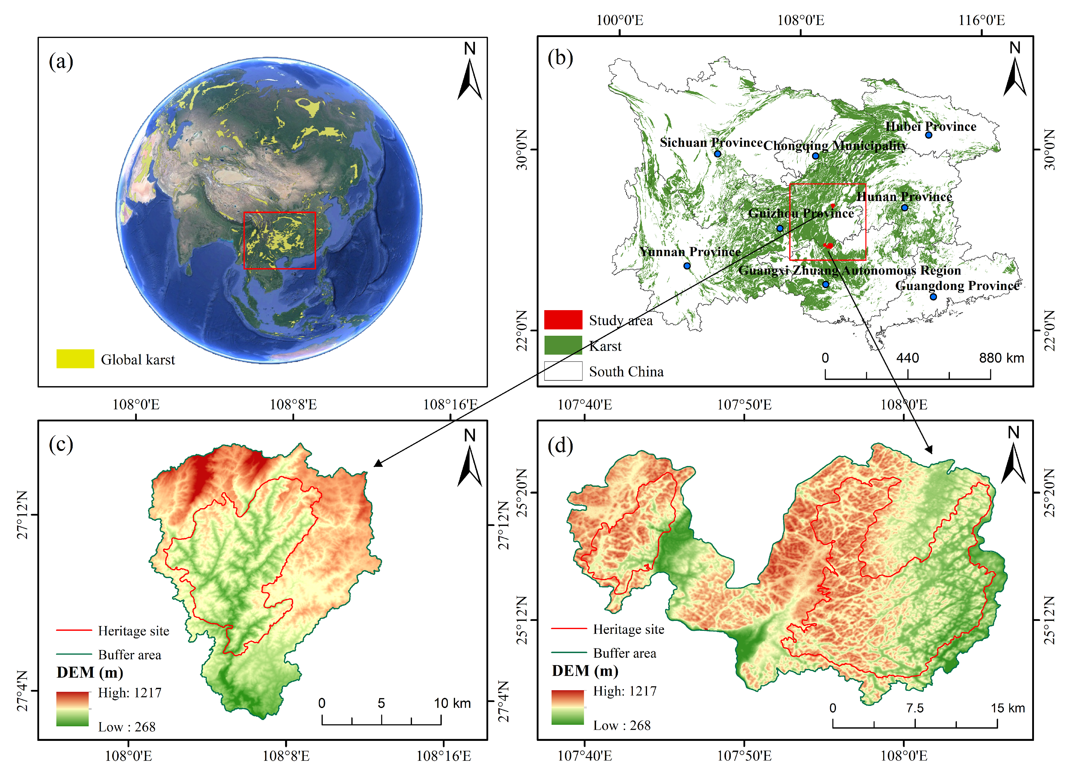
The Shibing Karst WNHS is located at Shibing County, Qiandongnan Prefecture, Guizhou Province (Figure 1), with an area of 282.98 km2 [22]. It is located within the humid climate zone with subtropical monsoon, characterized by a mild and humid climate. The average temperature throughout the year is around 16 °C, with annual precipitation of 1220 mm, and the average altitude of the area is 912 m [23]. The mean annual population density from 2000 to 2020 was 87.6852/km2, while the mean annual GDP is 13,523 ¥ per capita, with the majority of this figure derived from the tourism sector. he Shi Bing Karst is a superlative example of tropical-subtropical dolomite karst on the global scale [24]. Dolomite is a carbonate rock containing calcium and magnesium, which is less soluble than limestone. The distinctive peaks and gorges that have developed under such lithological conditions are a defining feature of the Shibing Karst WNHS.

Figure 1.
The geographical location map of the research is: (a) the location of karst in the eight provinces of southwest China in the global karst; (b) eight provinces in southwest China are located in karst; (c) Shibing Karst WNHS; and (d) Libo-Huanjiang Karst WNHS.
The Libo-Huanjiang Karst WNHS is located at the confluence of Libo County in Guizhou Province and Huanjiang County in Guangxi (Figure 1). It encompasses an area of 730.16 km2 [22], within the subtropical humid monsoon climate zone, with an average year-round temperature of approximately 15 °C and an average annual rainfall of 1752 mm, and the average elevation of the area is 758 m above sea level [25]. The mean annual population density from 2000 to 2020 was 62.0958/km2, while the mean annual GDP was 19,517 ¥ per capita, with the majority of this figure derived from the tourism sector. The Libo-Huanjiang Karst is a typical subtropical limestone cone-shaped karst landscape. It is the most typical example of the Peak Tree-Peak Forest Karst, which is an illustration of the evolution of similar karst landscapes across the globe. Concurrently, the Libo-Huanjian and Huanjiang karsts collectively constitute a vast and comprehensive subtropical cone-shaped karst World Heritage ecosystem, which offers an optimal environment for biological growth and reproduction [26].
2.2. Data Sources
This research examines the space–time changes in ESs and the trade-offs and synergistic relations at the Shibing Karst WNHS and the Libo-Huanjian Karst WNHS between the years 2000, 2010, and 2020.
In order to conduct research, it is necessary to have access to meteorological data, topographic and geomorphological data, and land use data (Table 1). Meteorological data encompass precipitation, temperature, and potential evapotranspiration, derived from spatial station records from the Meteorological Data Center of the China Meteorological Administration (CMA) and spatially interpolated using the Kriging method. Topographic and geomorphological data encompass soil data, digital elevation models (DEMs), and other relevant information. As raster data exhibit varying resolutions, inconsistent coordinates, or offsets, the study was standardized to raster data in order to accurately quantify the trade-offs and synergies among the various ESs and to ensure the scientific validity and accuracy of the study. In order to address the issue of differing resolutions, the resampling tool of ArcGIS10.2 was employed to standardize the resolution to 10 m by 10 m. In order to address the issue of the non-uniformity of coordinates and of coordinate shifts, a variety of geographic proofreading, projection, and other tools for coordinate standardization were employed. Due to the limited spatial extent of the study area, remote sensing images from 2000, 2010 and 2020 were employed as the principal data source. The analysis was conducted using ArcMap 10.2 and ENVI 5.3 software, employing supervised classification and a confidence interval of 95%. The results of the field validation, when considered alongside the findings of the land use interpretation, demonstrate that the latter is aligned with the current land use status of the study area.

Table 1.
Data source and processing methods.
2.3. Research Methodology
2.3.1. Cellular Automata (CA)-Markov Model
The CA-Markov model is a widely used tool for prediction of land use and land-cover change [25]. It combines the simulation advantages of the CA model with the temporal prediction advantages of the Markov model [27], enabling the evaluation and simulation of spatial and temporal changes in image elements [28]. Consequently, the CA-Markov model used in this paper to simulate the land-cover change of the Karst WNHS, thereby enabling an assessment of its ecological quality.
CA models are frequently employed to depict the space–time unfolding of intricate systems, and are hence designated as a local discrete-time network dynamics model [29]. The principle of calculation is as follows:
where S is the meta-cellular state, t and t + 1 are the corresponding meta-cellular moments, and n is the distance between the two instants [25].
The fundamental tenet of Markov modelling is the comparison of the subsequent state of affairs with that of the preceding state [30].
where and are the states at moments and . are the transfer matrix.
2.3.2. Water Conservation (WC)
Following the concept of the water balance, the use of InVEST simplifies the confluence process, without distinguishing between surface runoff, loamy runoff, and baseflow. It is assumed that the water produced by the grid reaches the water outlet through any of the aforementioned pathways [12].
where is the annual water production, is the annual average rainfall of grid cell x, and is the actual annual average evapotranspiration of grid cell x on land use type j [31] (Table S4 in the Supplementary Materials).
Given that the selected study areas in this paper are all mountainous, it is essential to consider the influence of topographic factors such as elevation and slope on the water-holding function. In order to achieve this, it is necessary to utilize topographic indices, soil saturated hydraulic conductivity, and flow rate coefficients in order to correct the water yield [32]. The final calculations yielded a water conservation which is as follows:
where Retention is the amount of WC, TI is the tectonic indicator, Ks is the soil saturated hydraulic conductivity, Velocity is the flow coefficient, and Yield is the annual water yield [33] (Figure S1 in the Supplementary Materials).
2.3.3. Soil Conservation (SC)
The sediment transport rate module of InVEST was used to assess conservation [34]. The calculation principle is as follows:
where is the amount of sediment retained by the grid (t) and is the amount of sediment intercepted by the grid upstream of the grid (t) (Table S4 in the Supplementary Materials).
2.3.4. Habitat Quality (HQ)
The HQ component of InVEST was applied to evaluate the level of biodiversity, with the HQ Index serving to indicate the quality of habitats within a given area [35]. The index is a function of the intensity of the impact of the stressor (Table S1 in the Supplementary Materials), the sensitivity of the habitat to the stressor (Table S2 in the Supplementary Materials), the distance of the habitat from the stressor, and the degree of the legal protection of the land [36].
where and are the HQ and the level of stress suffered by grid x in habitat type j, respectively; is the habitat suitability index; z is the normalized constant; and k is the semi-inclusive sum constant [37].
2.3.5. Carbon Storage (CS)
InVEST employs a specific methodology for calculating carbon stocks. This methodology involves the creation of a table of the four major carbon pools, with vegetation type serving as the statistical unit (Table S3 in the Supplementary Materials). The four major pools are then aggregated for different land cover types, and finally, the carbon stock in a given area is determined [38].
where is the carbon stock in area x and is the range-of-land-use category j in zone x. represent the surface biomass, beneath the surface biomass, soil carbon sink, and dead organic matter carbon pool, respectively [39].
2.3.6. Spearman Correlation Coefficient
Correlation analyses are a common method of assessing interactions among ESs [40]. This paper investigates the synergies and trade-offs among ESs in the region using correlation analysis. Spearman’s correlation is a non-parametric method of statistical analysis, and geographic data are non-linear and non-normally distributed [40].
where stands for the Spearman correlation coefficient between and . and denote the land cover function. Xi and Yi in the space unit i. n denote the quantities of space units [41]. When > 0, the two services are positively correlated and synergistic; conversely, when < 0, the decrease in one type of ES is negatively correlated with an increase in the other type of ES and is a trade-off [42].
2.3.7. Bivariate Spatial Autocorrelation Model
Spatial correlation analysis is used to determine and evaluate patterns of spatial correlation, with the objective of detecting heterogeneity or convergence in spatial data. This encompasses the application of Global Moran’I and Local Moran’I [43].
(1) Global spatial autocorrelation is employed to estimate the overall level of linkage, significance, and geographical spread of ESs across all study units within the study area [4]. Moran’s I range if I > 0 indicates that the spatial distribution of ESs is positively correlated and that there is a ‘high-high’ or ‘low-low’ aggregation phenomenon; if I = 0, it indicates that the grid units are randomly distributed in space; if I < 0, it means that the ESs are negatively correlated in space, and that there is the phenomenon of a ‘high-and-low’ or a ‘low-and-high’ neighborhood [44].
where I is the global autocorrelation Moran index; and denote the ESV values of the ith and jth spatial grid cell, respectively; is the average value of ESV of the evaluated grid cell; is the weight matrix established based on the spatial grid adjacency; and n is the number of grids of the spatial cell.
(2) Local spatial autocorrelation is a statistical technique that can be employed to test the spatial correlation and spatial heterogeneity of ES functions across local regions [45]. Furthermore, the bivariate LISA (Local Indicators of Spatial Association) distribution map was used to characterize the correlation among ESs within the study area [41]. The calculation principle is as follows:
where denotes the local spatial autocorrelation Moran index; and are the ESV values of the and spatial cells, respectively; denotes the average value of the ESV of the lattice grid; and and n have the same meanings as in Equation (9).
3. Results
3.1. Characteristics of Land Use Conversion
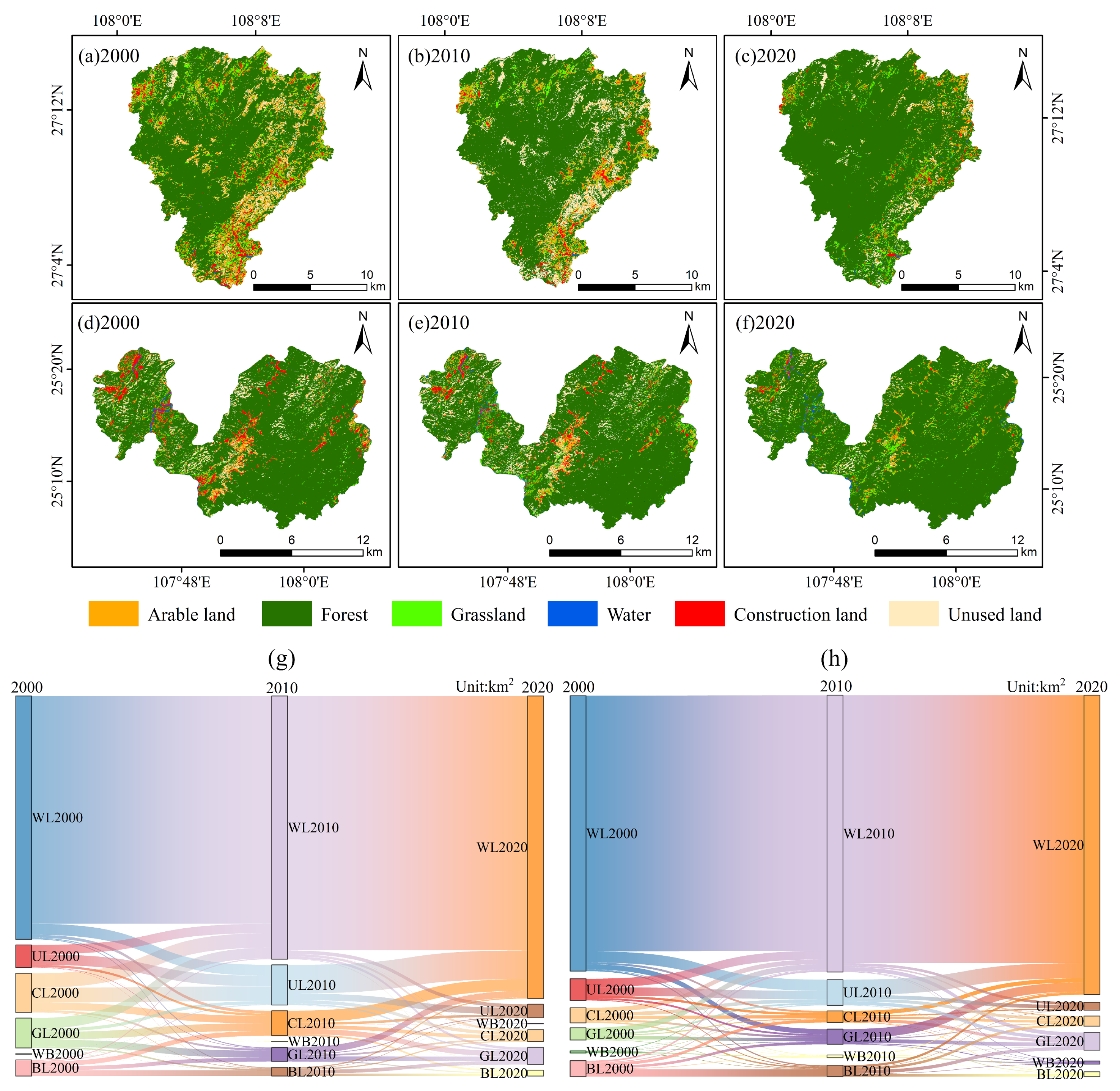
The following figures illustrate the land use spatial distribution map and modifications of the Shibing and the Libo-Huanjian between the years 2000 and 2020 (Figure 2). The predominant land use type of the Shibing Karst WNHS is woodland (WL), with the proportion of WL area fluctuating between 60% and 80% across the three periods. This is characterized by a wide range of distribution and a considerable area. The cropland (CL) and building land (BL) are primarily situated within the buffer zone and are distributed in blocks. In respect to the amount of change from 2000 to 2020, the area of WL exhibited the greatest change, with a cumulative increase of 47.76 km2. Unused land (UL) demonstrated a tendency to increase and then reduce, while the CL remained in decline. The range of grassland (GL), BL, and water (WB) areas did not change significantly.
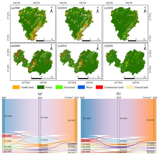
Figure 2.
Land cover maps of study area ((a–c) refer to the land use of the Shibing Karst WNHS in 2000, 2010, and 2020; (d–f) refer to the land use of the Libo-Huanjiang Karst WNHS in 2000, 2010, and 2020) and land use transfer matrix; (g) Shibing; (h) Libo-Huanjian.
The predominant land use type of the Libo-Huanjian Karst WNHS from 2000 to 2020 was WL. The proportion of WL area in all three periods ranged from 80% to 90%, with the distribution including the heritage site and the butterfly area. The remaining land types are primarily concentrated in the buffer zone in a linear distribution. In terms of inter-annual changes in the various types of areas from 2000 to 2020, the area of WL has undergone the most significant change, increasing by up to 54.92 km2. This is followed by UL, which has undergone a cumulative decrease of 34.48 km2. The majority of the UL has been transformed into GL and WL under the protection of localities, as evidenced by the spatial change map. The area of GL has exhibited a gradual increase, while the areas of CL and BL have shown a gradual decline. In contrast, the region of WB has exhibited minimal change.
The land use transfer matrix of the Shibing and the Libo-Huanjiang from 2000 to 2020 indicates that the majority of the transfer of the two study areas occurred between WL, followed by UL, BL and CL, with less transfer in and out of GL and WB areas. In summary, the Shibing and the Libo-Huanjiang are characterized by a high degree of WL resources.
3.2. Spatiotemporal Heterogeneity of ESs
3.2.1. Spatiotemporal Variations in ESs
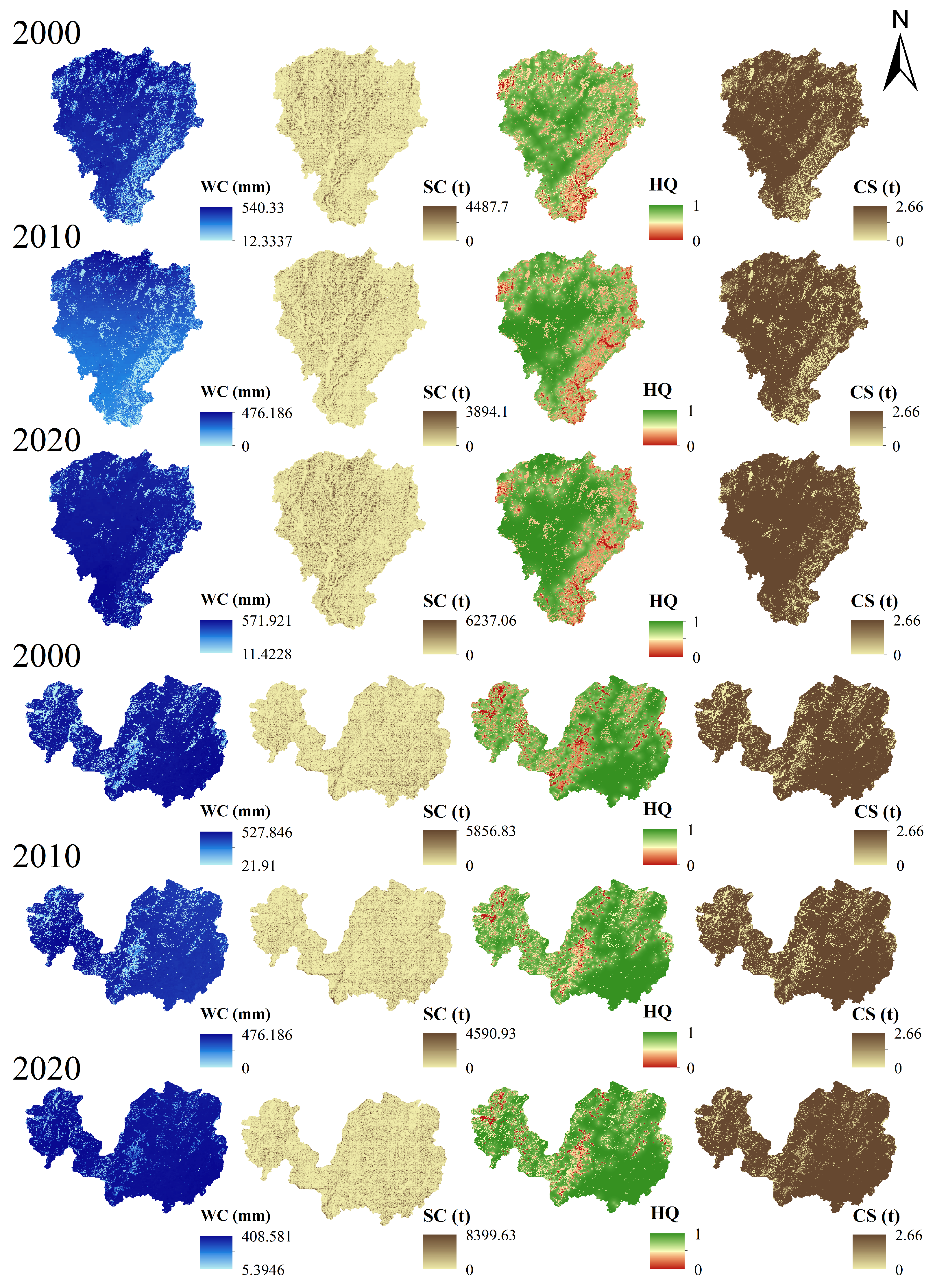
From 2000 to 2020, the WC of the Shibing Karst WNHS exhibited a general trend of increasing and then decreasing. The WC decreased from 540.33 mm in 2000 to 476.186 mm in 2010, and then increased to 571.921 mm in 2020. The SC demonstrated a general trend of decreasing and then increasing, with the WC decreasing from 4487.7 t/(km2·a) in 2000 to 4590.93 t/(km2·a) in 2010, and then increasing to 6237.06 t/(km2·a) in 2020. The HQ index demonstrated an upward trajectory, expected to grow by an average annual 9.89%. The mean value of HQ increased from 0.711 to 0.778 between 2000 and 2010, expected to grow by an average annual 4.63%. The mean value of HQ in the 2010–2020 period exhibited a continuous upward trend, reaching an average value of 0.851 by 2020. The CS change demonstrates a fluctuating pattern, with a downward trend followed by an upward one. The average rate of change of CS from 2000 to 2010 was −0.07%, with minimal fluctuations in the average value. In contrast, the average rate of change of CS from 2010 to 2020 was 7.03%, accompanied by a notable increase in the average value, reaching 2.4953 by 2020.
The WC of the Libo-Huanjiang Karst WNHS shows an overall decreasing trend from 2000 to 2020. The WC decreased from 527.846 mm in 2000 to 476.186 mm in 2010, and then it reduced to 408.581 mm in 2020. The SC demonstrated an overall decreasing trend, with an upward trend and then a trend of decline. The WC decreased from 5856.83 t/(km2·a) to 4590.93 t/(km2·a) in 2010, and then it increased to 8399.63 t/(km2·a) in 2020. The HQ trend is comparable to that of Shibing, exhibiting a gradual increase in the trend of its average annual increase of 1.849%. From 2000 to 2010, the HQ increased from 0.798 to 0.813, representing a growth rate of 1.86%. Similarly, from 2010 to 2020, the average value of HQ increased from 0.786 to 0.808, with an average annual increase of 1.82%. From 2010 to 2020, the average value of HQ continued to increase, reaching 0.885 by 2020. The CS changes exhibited a tendency to fall and then to rise again, with an average rate of change in carbon storage of −0.11 per cent from 2000 to 2010 and an average rate of change in CS of 5.39 per cent from 2010 to 2020, with the average value reaching 2.5059 by 2020.
With regard to the spatial distribution of WC and CS in the Shibing and the Libo-Huanjiang, the overall pattern has changed little. The high values are focused on the WNHS, while the low values are found in the construction land and the water areas in the buffer zones. The high values of HQ in the two study areas are concentrated in the woodland and grassland areas within the heritage sites and buffer zones. In contrast, the low values are primarily focused on the CL and BL areas. The high values of SC in the Shibing are concentrated in the northern region, with a gradual decrease in the south. In contrast, the SC in the Libo-Huanjiang is concentrated in the southeast, with a corresponding decrease in the south. The negative values are distributed primarily in the buffer zone (Figure 3).
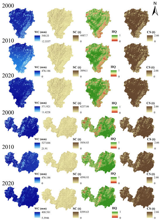
Figure 3.
Distribution of ESs in 2000, 2010, and 2020 (WC—Water conservation, SC—soil conservation, HQ—Habitat quality, CS—Carbon storage).
3.2.2. Changes in ESs Dynamics of Different Land Use Types
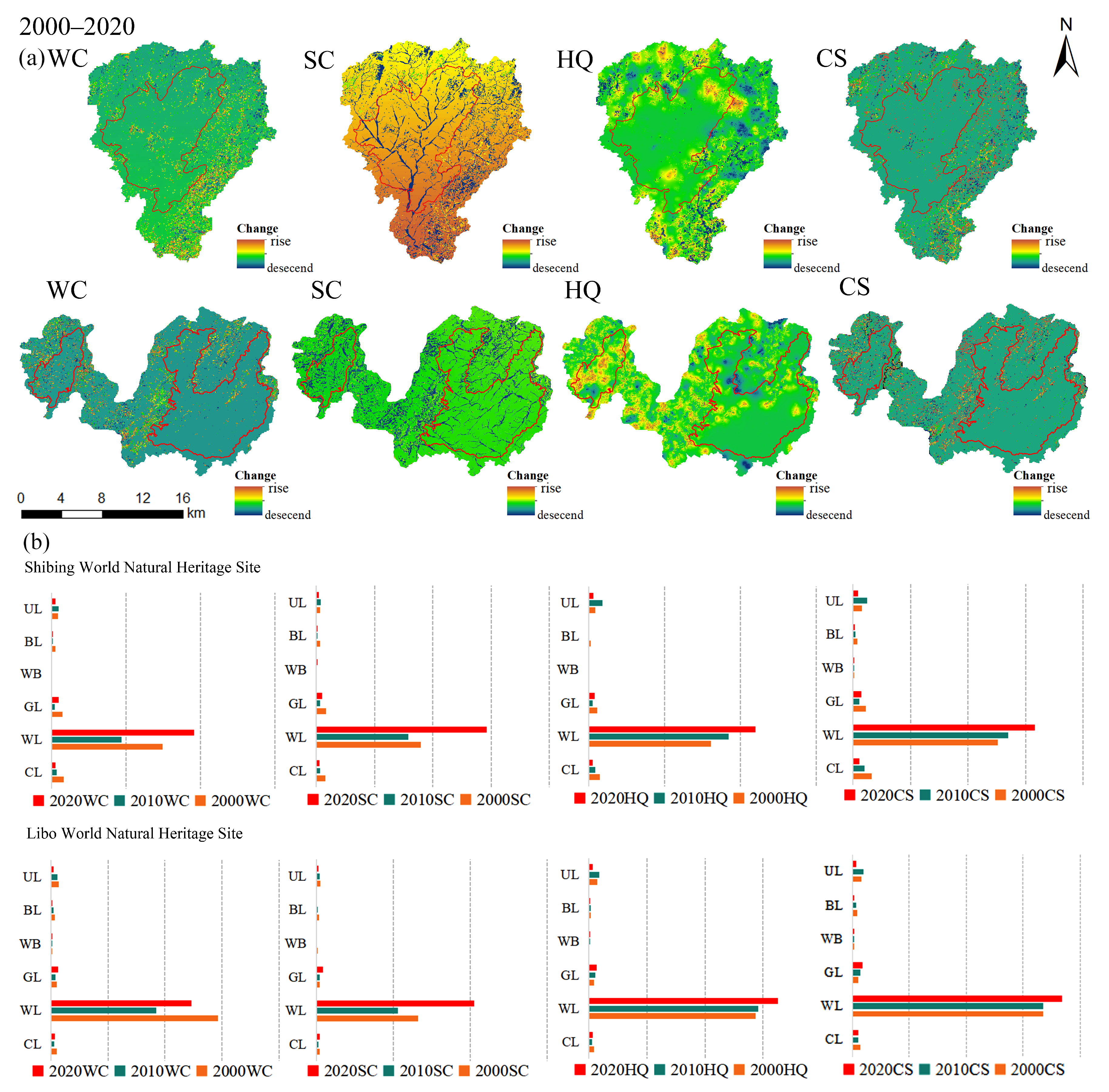
Over the past two decades, the WC, HQ, and CS of the Shibing Karst WNHS have demonstrated a general stability. The buffer zone has undergone a significant change and demonstrated a downward trend. In contrast, SC exhibited an upward trend, with a few areas displaying a linear downward trend. The land classes with the highest to lowest mean annual WC per unit area, in descending order, are as follows: WL, GL, CL, UL, BL, and WB. WC accounted for more than 70 per cent from 2000 to 2020, and for 89.59 per cent in 2020. WL, CL, GL, UL, BL, and WB are the land categories with the highest annual average SC per unit area, in descending order. The proportion of SC was above 80% from 2000 to 2020, and reached 93.16% in 2020. The ranking of the land categories by annual average HQ per unit area, from highest to lowest, are as follows: WL, GL, UL, CL, BL, and WB. WL accounted for more than 88 per cent from 2000 to 2020, with a peak of 91.43 per cent in 2020. In contrast, WB accounted for less than 1 per cent. The annual average CS per unit area is as follows, in descending order: WL, UL, CL, GL, BL, and WB. WL accounted for more than 70 per cent annually from 2000 to 2020, with all categories demonstrating a gradual growth trend.
Over the past two decades, the WC, HQ, SC, and CS of the Libo-Huanjiang Karst WNHS have demonstrated a consistent overall trend, with the SC exhibiting a linear decline in certain areas of the site. The different ESs exhibited a substantial decline in the buffer zone, demonstrating a block-like pattern of reduction. The land classes with the highest to lowest mean annual WC per unit area, in descending order, are as follows: WL, CL, GL, UL, BL, and WB. WC accounted for more than 80 per cent of the total from 2000 to 2020, and 90.16 per cent in 2020, while the other land categories accounted for less than 6 per cent of the total. The land categories, ranked from largest to smallest in terms of annual average SC per unit area, are as follows: WL, CL, GL, UL, BL, and WB. The proportion of SC from 2000 to 2020 was above 80%, reaching 93.16% and 92.25% in 2020. The annual average HQ per unit area, in descending order, are as follows: WL, UL, CL, GL, BL, and WB. WL accounted for more than 80% from 2000 to 2020, with a peak of 91.24% in 2020. This demonstrates a sustained growth trend over the past 20 years. The annual average CS per unit area is, in descending order, WL, UL, GL, CL, BL, and WB. WL accounted for more than 70% of the total annually from 2000 to 2020, with all categories demonstrating a gradual growth trend.
It can be observed that different land cover types are capable of providing different types of ESs. In this study, the four services WC, SC, HQ, and CS are further analyzed from the perspective of land cover types. Annual average WC and SC per unit area of different land cover types in the Shibing Karst WNHS and the Libo-Huanjiang Karst WNHS exhibited considerable variation, particularly between forest land and other land cover (Figure 4).
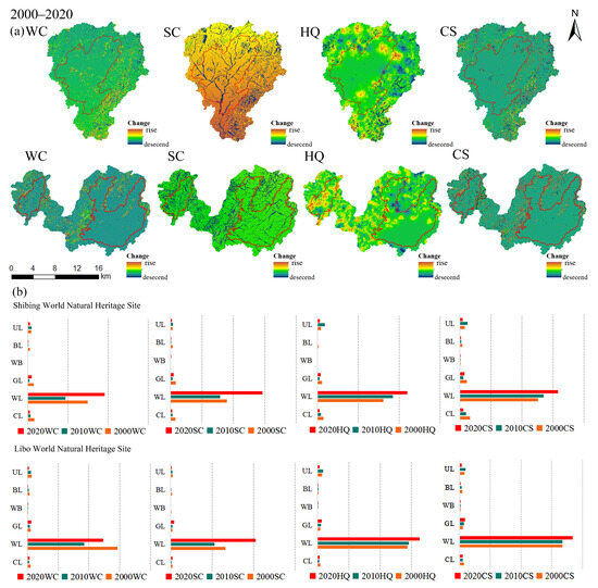
Figure 4.
(a) Characteristics of changes in different ESs, (b) bar chart of six land cover types for years 2000, 2010, and 2020.
3.3. ESs Trade-Offs/Synergies
3.3.1. Spearman Correlation Coefficients between ESs
Among the six pairs of ESs in the Shibing Karst WNHS, WC and CS exhibited a highly correlated relationship (r ≥ 0.5), indicative of a strong synergistic effect, with a mean value of a correlation coefficient of 0.88. WC exhibited a weak synergistic relationship with HQ, while HQ demonstrated a similarly weak synergistic relationship with CS. The mean correlations are 0.38 and 0.37. Additionally, a weak trade-off was observed among WC and SC, HQ and SC, and CS and SC. The mean values of the correlation coefficients are as follows: −0.074, −0.076, and −0.15 (Figure 5).
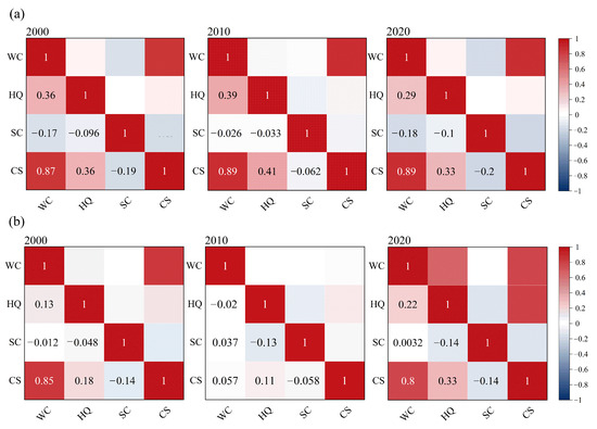
Figure 5.
Spearman’s rank correlation coefficients of pairs of ESs in 2000, 2010, and 2020. (a) Shibing Karst WNHS. (b) Libo-Huanjiang Karst WNHS.
Among the six pairs of ESs in the Libo-Huanjiang Karst WNHS, WC and CS in 2000 and WC and CS in 2020 were all in strong synergistic relationships; the coefficients are 0.85 and 0.8, respectively. WC and HQ in 2000 and HQ and CS were all in weak synergistic relationships, with correlation coefficients of 0.13 and 0.18. WC and SC, HQ and SC, and CS and SC are all weak compromises. The coefficients are −0.012, −0.048, and −0.14. In 2010, CS and WC, SC and WC, and HQ and CS were all weakly synergistic, with coefficients of 0.057, 0.037, and 0.11. WC and HQ, SC and HQ, and CS and SC are all weak trade-offs; the coefficients are −0.02, −0.13, and −0.058, respectively. In 2020, WC had a weak synergistic relationship with SC, and HQ had a weak trade-off relationship with SC, and SC had a weak trade-off relationship with HQ, with SC, and with CS; the coefficients are 0.0032, −0.14, and −0.14 (Figure 5).
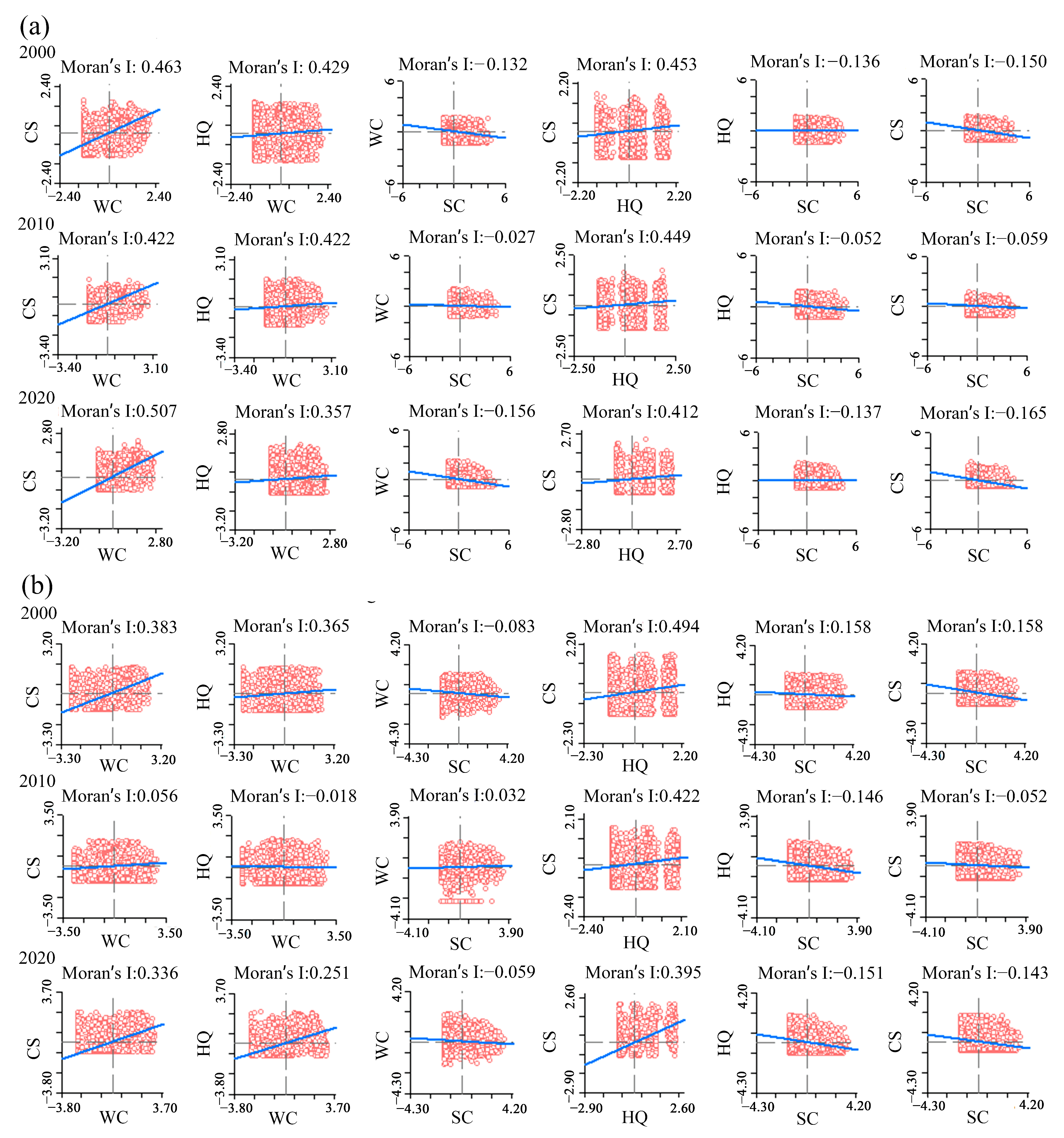
3.3.2. Moran’s Index between ESs
The scatterplot is divided into four quadrants, and each is centred on the mean value (Figure 6). The statistical analysis of each quadrant revealed that the two study area points in the graph are primarily distributed in quadrants 1 and 2. Among the indices, the global autocorrelation indices of CS and WC, HQ and WC, and HQ and CS of the Shibing from 2000 to 2020 were significantly positive at the level of 0.05. This indicates a positive spatial correlation, indicating synergy among the ESs. Furthermore, the synergistic strengths of WC and CS and of WC and HQ are decreasing and then increasing, while the synergistic strengths of HQ and CS are continuously increasing. The global autocorrelation indices of SC with WC, SC with HQ, and SC with CS are significantly negative at the level of 0.05, indicating a negative spatial autocorrelation. This suggests that the ESs are in a trade-off. The strength of the trade-offs between SC and WC and SC and CS is weakened and then strengthened, while the strength of the trade-offs between SC and HQ is strengthened and then weakened. In 2020, the strength of the trade-offs between SC and HQ reached a synergistic state, as indicated by the Moran’s index, which is −0.005.
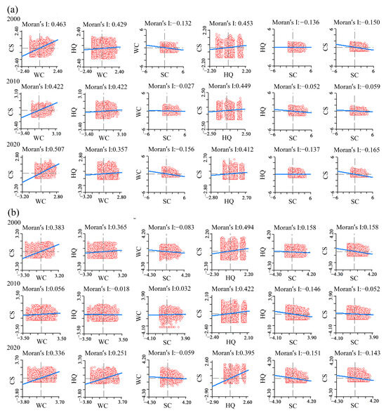
Figure 6.
Moran’s I index of trade-offs and synergies between ESs. (a) Shibing Karst WNHS. (b) Libo-Huanjiang Karst WNHS.
The global autocorrelation indices of WC and CS and of HQ and CS in the Libo-Huanjiang Karst WNHS exhibited a positive association at the 0.05 level during the period of 2000–2020. This indicates a positive spatial correlation, which suggests a synergistic relationship between the services. The synergistic relationship between WC and CS tended to decrease and then increase, while the relationship between HQ and CS gradually increased during the period of 2000–2020 In contrast, SC and HQ show a trade-off, with the level of trade-off gradually increasing. A positive spatial correlation has been identified between WC and CS, which suggests a synergistic relationship between the two services.
3.3.3. Spatial Representation of Trade-Offs and Synergistic Relationships for ESs
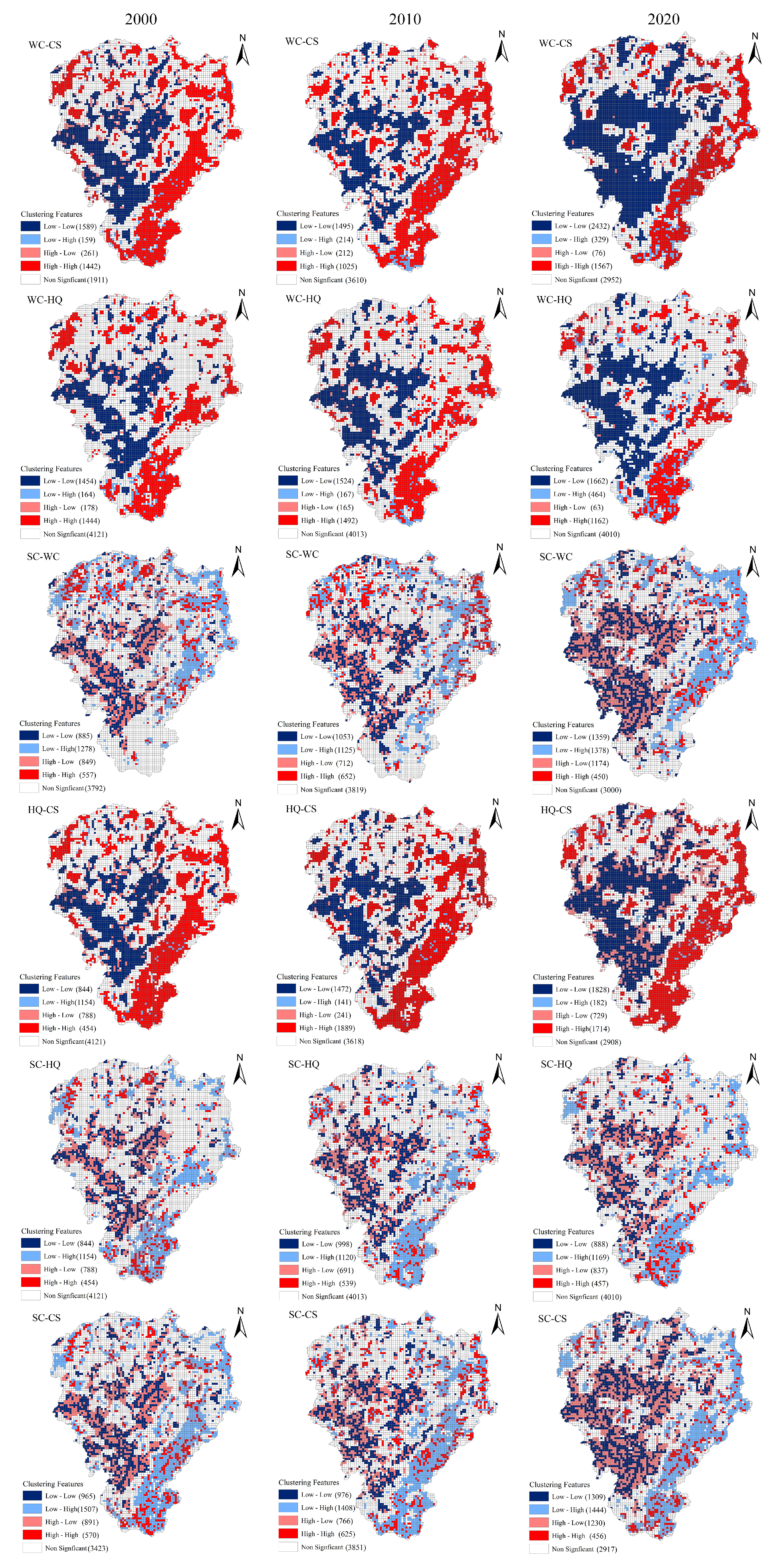
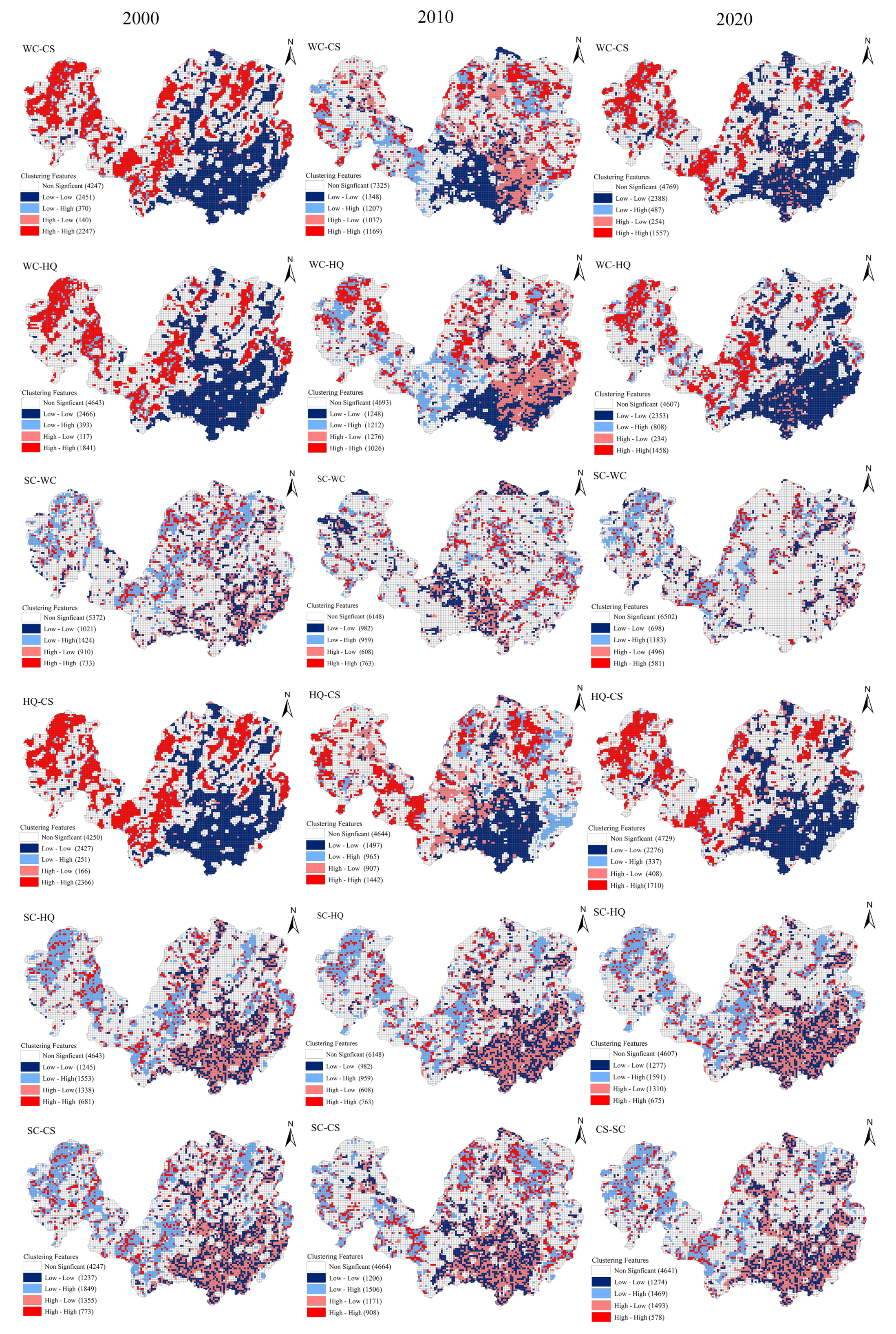
The results indicate that (Figure 7), among the six pairs of ESs in the Shibing Karst WNHS, the synergies between CS and WC, HQ and WC, and HQ and CS was more significant. Furthermore, the low-low clusters were mainly distributed within WNHS. The high-low aggregation area is focused on the cultivated land and the construction land regions. The spatial distribution of the high-first aggregation and low-high aggregation in the trade-off relationship among SC and WC, SC and HQ, and SC and CS is more dispersed. Among the three pairs of services, the spatial spread of the trade-off in 2020 exhibited the widest scope of distribution and the largest number of occurrences.

Figure 7.
Spatial distribution of trade-offs and synergies between ESs at the Shibing Karst WNHS.
Among the six pairs of ESs in the Libo-Huanjiang Karst WNHS (Figure 8), the synergy between WC and HQ and between HQ and CS is more significant. The low-low clustering is mainly distributed in the part of the Huanjiang Protected Area in a block-like distribution, while the high-high clustering is mainly distributed in the buffer zone of arable land, construction land, and unused land area in a shape-like distribution. The SC and WC, SC and HQ, and SC and CS Weighing Guanzhong high and low clusters are concentrated in the core region of the Huanjiang WNHS, with the low and high clusters primarily situated in the Libo buffer zone.

Figure 8.
Spatial distribution of trade-offs and synergies between ESs at the Libo-Huanjiang Karst WNHS.
4. Discussion
4.1. Spatial and Temporal Changes in Land Use and ESs
In recent years, the delicate karst ecosystem has undergone significant alterations to the karst landscapes, which have been caused by both climate change and human activities [15]. Nevertheless, land-cover change also has a direct influence on the temporal development and the spatial extent of ESs [46]. This paper employs a spatio-temporal analysis of ESs in the Shibing and Libo-Huanjiang Karst WNHS. The findings indicate that WC is related to precipitation, soil depth, and the available water content of vegetation. The heritage site is predominantly forest and grassland, with fertile soil and a high vegetation cover, resulting in greater soil depth and vegetation-available water content than the buffer zone. Consequently, the spatial distribution of WC is more prevalent in heritage sites than in buffer zones. Changes in the area of woodland and grassland also have a major impact on soil retention [47]. The interception of rainfall by woodland and grassland can be attributed to the forest canopy, the leaf litter, and to the grassland layer on the soil surface. This phenomenon reduces the direct scouring of the soil by rainwater, thereby increasing SC. These results are in accordance with those previously reported by Chen et al. [48].
A multitude of researchers have demonstrated that land-cover change has a profound impact on the structure, the characteristics, and the processes of ecosystems [49,50,51]. The CS in the region area was primarily focused on land classes with high vegetation cover, such as WL and GL. WL, as the land category with the highest CS among all land categories, demonstrated a significant increase in CS with the expansion of the WL area. These findings align with those of previous studies, including those by Qiao et al. [10] and Yuan et al. [52]. The HQ index is primarily indicative of the local ecological status and degree of biodiversity [53]. The buffer zone within the study area is predominantly composed of CL and BL, which are not conducive to the survival of organisms. Consequently, the HQ is relatively low. The HQ was higher in the heritage site due to the presence of WL, GL, and other ecological land types, which provided an optimal environment for the survival of organisms. These results are in accordance with those previously reported by Lin et al. [54] and Cui et al. [55]. In summary, the reduction in CL and BL and the increase in WL between the years 2000 and 2020 have resulted in an overall increase in CS and HQ. Consequently, alterations in land cover structure will predominantly give rise to analogous alterations in Ess’ functions.
4.2. Trade-Offs/Synergies of ESs
The innovation of this research lies in the application of the Spearman correlation coefficient to calculate ES trade-offs and synergies. This approach has been validated both in general and spatially using bivariate and local Moran’I indices, which have proven to be highly accurate. The correlation calculated by the Moran’I index was found to exhibit a certain lag, which reflected the ES’s trade-offs and synergies in a more realistic and comprehensive manner. The WC and the SC are significantly affected by precipitation. In contrast, the HQ and the CS are strongly influenced by land use change [56]. The extensive and continuous growth in the region of woodland in the research region, which has more than 75% vegetation cover, contributed to the improvement of HQ and CS. This resulted in a synergy between HQ and WC, CS and WC, and HQ and CS, which is more consistent with the results of existing studies [57]. The monoculture of vegetation in the core area, which is mainly forested, and the high distribution of BL and CL in the buffer zone, resulted in the uneven rain erosion resistance of the soil in the study area. This, in turn, indirectly affected the SC capacity, in accordance with the findings of Chang et al. [58] and Tian et al. [59]. Furthermore, ESs exhibit scale effects [60]. The outcomes of trade-offs and synergies can be influenced by a number of factors, including spatio-temporal heterogeneities, natural environmental factors, and socio-economic conditions.
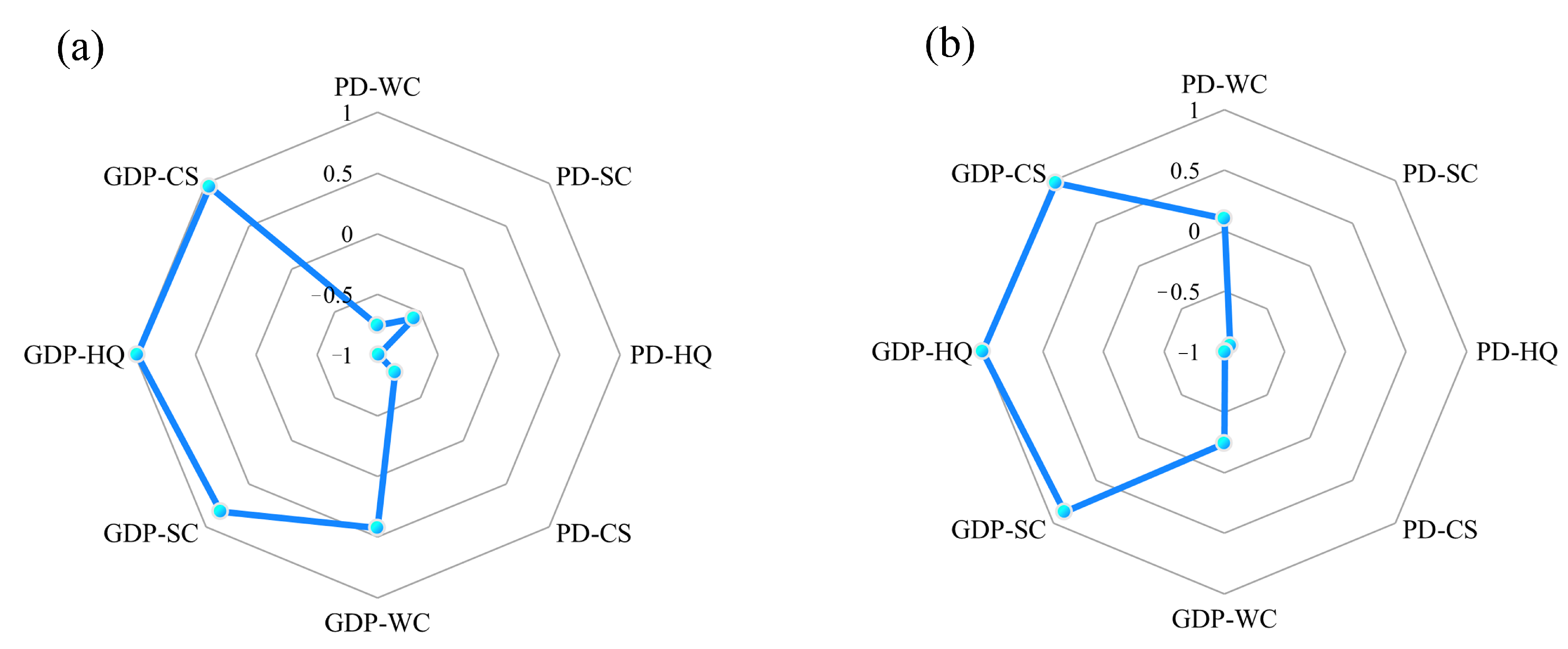
An increase in population density and the clustering of economic activities results in a notable surge in demand for ecosystem services, which in turn precipitates ecosystem degradation and a reduction in the supply of ESs [61]. The implementation of appropriate regulatory measures to control the intensity of human activities is conducive to the synergistic development of ecosystem services. The Shibing Karst WNHS and the Libo Karst WNHS both demonstrate a negative correlation between population density and various ecosystem services, as well as a positive correlation between GDP and each ecosystem service (Figure 9). The results indicated that population density and GDP exhibited the most significant correlations with soil conservation, habitat quality, and carbon storage, with correlation coefficients exceeding 0.5. An increase in population density is associated with a reduction in ecosystem services. This illustrates the importance of considering the spatial variability of ecosystem services in response to changes in socio-economic factors. In the future, changes in different ecosystem services can be studied using longer-time-span data and regionally varying socio-economic parameters, thus providing a more comprehensive understanding of the factors influencing these services.
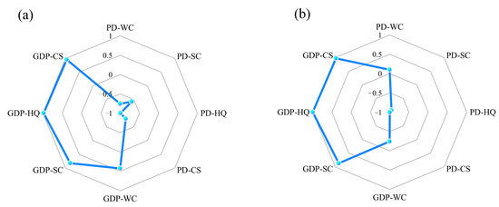
Figure 9.
Population density and GDP in relation to different ecosystem services. (a) Shibing Karst WNHS. (b) Libo-Huanjiang Karst WNHS.
4.3. Limitations and Prospects
This research analyses the changes that have occurred in the Karst WNHS over a period of thirty years. The conclusions reached will have certain reference value for the more detailed examination of the relationship between ESs in the study area. However, there may be some differences compared with the long-term series of spatial and temporal dynamics studies. In the future, we will select continuous time scale data to conduct a multi-year continuous change study in order to reduce the uncertainty. Furthermore, the influence of precipitation, temperature, and topography on ESs is more complex. In the future, we will investigate the factors and mechanisms that drive the different ESs in depth, thus providing a foundation for the optimization of the distribution of land cover and the sustainable development of ecological and economic ecosystems in the Karst WNHS in the future.
As a globally significant ecological functional area, the objective of this paper is to propose a framework for promoting synergistic relationships among ESs within the site and to enhance the optimization of the ecological environment. This framework is based on the results of the research conducted on the Karst WNHS:
- (1)
- Rationalize the planning of land use types; continue to implement ecological conservation projects, for example restoring farmland to woodland and grasslands; and relocate some of the arable and building land to the townships around the buffer zone, with the objective of enhancing the overall ecological suitability of the heritage site and improving the sustainability of its ecosystem;
- (2)
- The objective is to optimize zoning management, to manage the existing heritage sites and buffer zones in a zoning pattern, and to integrate them with the space–time distribution of ESs and the spatial pattern of global trade-offs and synergies, as assessed in the present study. Furthermore, targeted zoning management and protection of the ecological service areas that require upgrading and the areas of the main trade-offs and relationships will be carried out. This will facilitate the ecological protection of the Karst Natural WNHS, while also contributing to global sustainable development.
5. Conclusions
In order to enhance the regional ESs’ provisioning capacity, to mitigate conflicts between Ess, and to achieve the sustainable development of WNHS, it is crucial to investigate the synergies and trade-offs among ESs in the Karst WNHS. In this research, the InVEST model was used to assess the four key ESs in the Shibing Karst WNHS and the Libo-Huanjiang Karst WNHS between the years 2000 and 2020. The changes in the development of ESs in different land use types were identified by histograms. The trade-offs and synergies among the ESs were analyzed with Sperman correlation analysis and a bivariate spatial autocorrelation model, and the following conclusions were reached:
(1) The inter-annual changes in WC and SC in the Shibing WNHS show considerable variability, displaying a declining and then increasing trend. At the Libo-Huanjiang WNHS, there is a gradual decrease in WC, a decrease followed by an increase in SC, and an uninterrupted increase in HQ and CS;
(2) The distribution of high-and low-value areas for ESs is closely linked to land use patterns. The WNHS is characterized by a high degree of vegetation and a rich biodiversity, which represents the high value area of each service. The buffer zone comprises CL, UL, and BL, which collectively represent the low value distribution area for each service. It has been demonstrated that WL represents the most critical land type in the development of ESs in the study area, with the greatest contribution to each service;
(3) A significant correlation was observed between changes in population density and GDP and changes in ecosystem services. The strongest correlations were found between population density and GDP and soil conservation, habitat quality, and carbon storage;
(4) The trade-offs and synergies among ESs were relatively stable, with the exception of WC and SC, which exhibited considerable fluctuations over time. There are significant synergistic relationships between CS and WC, HQ and WC, and HQ and CS in terms of their spatial distribution. Conversely, there are significant trade-offs among SC and WC, HQ and SC, and SC and CS in terms of their spatial distribution.
The clarification of the trade-offs and synergies among ESs and their spatial distribution represents the foundation for an examination of the ES’s changes in natural World Heritage sites. This investigation will facilitate the macro-control of natural resources in the sites and will serve as a reference point for the designation of a coordinated development strategy for resources and the environment in the natural World Heritage sites around the globe.
Supplementary Materials
The following supporting information can be downloaded at: https://www.mdpi.com/article/10.3390/land13091391/s1.
Author Contributions
M.F. and K.X. designed the study. M.F. collected the database and performed the research, analyzed data, and wrote the paper. Y.C. participated in data processing and model calculation. The remaining authors contributed to discussing the results and revising the manuscript. All authors have read and agreed to the published version of the manuscript.
Funding
This research was supported by the National Key Research and Development Program of China (2022YFF1300703), the Guizhou Provincial Key Technology R&D Program (No. 220 2023 QKHZC), and the Chinese Government-UNESCO World Heritage Protection and Development Program (No. 12 2018 GNTL TS).
Data Availability Statement
The data supporting the findings of this study are available from the corresponding author upon reasonable request.
Acknowledgments
We would like to thank the anonymous reviewers for their constructive comments, which improved the quality of this manuscript.
Conflicts of Interest
The authors declare no conflicts of interest.
References
- Costanza, R.; d’Arge, R.; De Groot, R.; Farber, S.; Grasso, M.; Hannon, B.; Limburg, K.; Naeem, S.; O’neill, R.V.; Paruelo, J. The value of the world’s ecosystem services and natural capital. Nature 1997, 387, 253–260. [Google Scholar] [CrossRef]
- Wong, C.P.; Jiang, B.; Kinzig, A.P.; Lee, K.N.; Ouyang, Z. Linking ecosystem characteristics to final ecosystem services for public policy. Ecol. Lett. 2015, 18, 108–118. [Google Scholar] [CrossRef]
- Bennett, E.M.; Peterson, G.D.; Gordon, L.J. Understanding relationships among multiple ecosystem services. Ecol. Lett. 2009, 12, 1394–1404. [Google Scholar] [CrossRef]
- Costanza, R.; de Groot, R.; Sutton, P.; van der Ploeg, S.; Anderson, S.J.; Kubiszewski, I.; Farber, S.; Turner, R.K. Changes in the global value of ecosystem services. Glob. Environ. Change 2014, 26, 152–158. [Google Scholar] [CrossRef]
- Rodríguez, J.P.; Beard, T.D.; Bennett, E.M.; Cumming, G.S.; Cork, S.J.; Agard, J.; Dobson, A.P.; Peterson, G.D. Trade-offs across Space, Time, and Ecosystem Services. Ecol. Soc. 2006, 11, 110128. [Google Scholar] [CrossRef]
- Adeyemi, O.; Chirwa, P.W.; Babalola, F.D.; Chaikaew, P. Detecting trade-offs, synergies and bundles among ecosystem services demand using sociodemographic data in Omo Biosphere Reserve, Nigeria. Environ. Dev. Sustain. 2021, 23, 7310–7325. [Google Scholar] [CrossRef]
- Foley, J.A.; DeFries, R.; Asner, G.P.; Barford, C.; Bonan, G.; Carpenter, S.R.; Chapin, F.S.; Coe, M.T.; Daily, G.C.; Gibbs, H.K.; et al. Global Consequences of Land Use. Science 2005, 309, 570–574. [Google Scholar] [CrossRef] [PubMed]
- Liu, Q.; Qiao, J.; Li, M.; Huang, M. Spatiotemporal heterogeneity of ecosystem service interactions and their drivers at different spatial scales in the Yellow River Basin. Sci. Total Environ. 2024, 908, 168486. [Google Scholar] [CrossRef]
- Howe, C.; Suich, H.; Vira, B.; Mace, G.M. Creating win-wins from trade-offs? Ecosystem services for human well-being: A meta-analysis of ecosystem service trade-offs and synergies in the real world. Glob. Environ. Change 2014, 28, 263–275. [Google Scholar] [CrossRef]
- Qiao, X.; Gu, Y.; Zou, C.; Xu, D.; Wang, L.; Ye, X.; Yang, Y.; Huang, X. Temporal variation and spatial scale dependency of the trade-offs and synergies among multiple ecosystem services in the Taihu Lake Basin of China. Sci. Total Environ. 2019, 651, 218–229. [Google Scholar] [CrossRef]
- Lang, Y.; Song, W. Trade-off Analysis of Ecosystem Services in a Mountainous Karst Area, China. Water 2018, 10, 300. [Google Scholar] [CrossRef]
- Qiao, Y.; Zhang, H.; Han, X.; Liu, Q.; Liu, K.; Hu, M.; Pei, W. Exploring drivers of water conservation function variation in Heilongjiang Province from a geospatial perspective. Acta Ecol. Sin. 2023, 43, 2711–2721. [Google Scholar] [CrossRef]
- Li, Y.; Luo, H. Trade-off/synergistic changes in ecosystem services and geographical detection of its driving factors in typical karst areas in southern China. Ecol. Indic. 2023, 154, 110811. [Google Scholar] [CrossRef]
- Naidoo, R.; Balmford, A.; Costanza, R.; Fisher, B.; Green, R.E.; Lehner, B.; Malcolm, T.; Ricketts, T.H. Global mapping of ecosystem services and conservation priorities. Proc. Natl. Acad. Sci. USA 2008, 105, 9495–9500. [Google Scholar] [CrossRef]
- Wang, K.; Zhang, C.; Chen, H.; Yue, Y.; Zhang, W.; Zhang, M.; Qi, X.; Fu, Z. Karst landscapes of China: Patterns, ecosystem processes and services. Landsc. Ecol. 2019, 34, 2743–2763. [Google Scholar] [CrossRef]
- Xiao, B.; Bai, X.; Zhao, C.; Tan, Q.; Li, Y.; Luo, G.; Wu, L.; Chen, F.; Li, C.; Ran, C.; et al. Responses of carbon and water use efficiencies to climate and land use changes in China’s karst areas. J. Hydrol. 2023, 617, 128968. [Google Scholar] [CrossRef]
- Xiong, K.; Chen, D.; Zhang, J.; Gu, X.; Zhang, N. Synergy and regulation of the South China Karst WH site integrity protection and the buffer zone agroforestry development. Herit. Sci. 2023, 11, 218. [Google Scholar] [CrossRef]
- Zhang, S.; Xiong, K.; Fei, G.; Zhang, H.; Chen, Y. Aesthetic value protection and tourism development of the world natural heritage sites: A literature review and implications for the world heritage karst sites. Herit. Sci. 2023, 11, 30. [Google Scholar] [CrossRef]
- He, L.; Zhang, J.; Yu, B.; Hu, M.; Zhang, Z. Assessment of ecosystem health and driving forces in response to landscape pattern dynamics: The Shibing Karst world natural heritage site case study. Herit. Sci. 2024, 12, 182. [Google Scholar] [CrossRef]
- Zhang, J.; Xiong, K.; Liu, Z.; He, L. Research progress on world natural heritage conservation: Its buffer zones and the implications. Herit. Sci. 2022, 10, 102. [Google Scholar] [CrossRef]
- Xiong, K.; Deng, X.; Zhang, S.; Zhang, Y.; Kong, L. Forest Ecosystem Service Trade-Offs/Synergies and System Function Optimization in Karst Desertification Control. Plants 2023, 12, 2376. [Google Scholar] [CrossRef] [PubMed]
- Liu, Q.; Wang, J.; Xiong, K.; Gong, L.; Chen, Y.; Yang, J.; Xiao, H.; Bai, J. Quantitative assessment of ecological assets in the world heritage karst sites based on remote sensing: With a special reference to South China Karst. Herit. Sci. 2024, 12, 129. [Google Scholar] [CrossRef]
- Bai, Y.; He, Q.; Liu, Z.; Wu, Z.; Xie, S. Soil nutrient variation impacted by ecological restoration in the different lithological karst area, Shibing, China. Glob. Ecol. Conserv. 2021, 25, e01399. [Google Scholar] [CrossRef]
- Liu, Q.; Gu, Z.; Lu, Y.; Xiao, S.; Li, G. Weathering processes of the dolomite in Shibing (Guizhou) and formation of collapse and stone peaks. Environ. Earth Sci. 2015, 74, 1823–1831. [Google Scholar] [CrossRef]
- Zhang, N.; Xiong, K.; Zhang, J.; Xiao, H. Evaluation and prediction of ecological environment of karst world heritage sites based on google earth engine: A case study of Libo–Huanjiang karst. Environ. Res. Lett. 2023, 18, 034033. [Google Scholar] [CrossRef]
- Xiong, K.; Zhang, S.; Fei, G.; Jin, A.; Zhang, H. Conservation and Sustainable Tourism Development of the Natural World Heritage Site Based on Aesthetic Value Identification: A Case Study of the Libo Karst. Forests 2023, 14, 755. [Google Scholar] [CrossRef]
- Gao, Y.; Wang, J.; Zhang, M.; Li, S. Measurement and prediction of land use conflict in an opencast mining area. Resour. Policy 2021, 71, 101999. [Google Scholar] [CrossRef]
- Wang, H.; Stephenson, S.R.; Qu, S. Modeling spatially non-stationary land use/cover change in the lower Connecticut River Basin by combining geographically weighted logistic regression and the CA-Markov model. Int. J. Geogr. Inf. Sci. 2019, 33, 1313–1334. [Google Scholar] [CrossRef]
- Zhao, Y.; Jia, X.; Liu, J.; Liu, G. Analysis and forecast of landscape pattern in Xi’an from 2000 to 2011. Acta Ecol. Sin. 2013, 33, 2556–2564. [Google Scholar] [CrossRef]
- Zhou, L.; Dang, X.; Sun, Q.; Wang, S. Multi-scenario simulation of urban land change in Shanghai by random forest and CA-Markov model. Sustain. Cities Soc. 2020, 55, 102045. [Google Scholar] [CrossRef]
- Guo, R.; Wu, T.; Liu, M.; Huang, M.; Stendardo, L.; Zhang, Y. The Construction and Optimization of Ecological Security Pattern in the Harbin-Changchun Urban Agglomeration, China. Int. J. Environ. Res. Public Health 2019, 16, 1190. [Google Scholar] [CrossRef] [PubMed]
- Li, M.; Liang, D.; Xia, J.; Song, J.; Cheng, D.; Wu, J.; Cao, Y.; Sun, H.; Li, Q. Evaluation of water conservation function of Danjiang River Basin in Qinling Mountains, China based on InVEST model. J. Environ. Manag. 2021, 286, 112212. [Google Scholar] [CrossRef] [PubMed]
- Yan, X.; Cao, G.; Cao, S.; Yuan, J.; Zhao, M.; Tong, S.; Li, H. Spatiotemporal variations of water conservation and its influencing factors in the Qinghai Plateau, China. Ecol. Indic. 2023, 155, 111047. [Google Scholar] [CrossRef]
- Han, H.; Yin, C.; Zhang, C.; Gao, H.; Bai, Y. Response of trade-offs and synergies between ecosystem services and land use change in the Karst area. Trop. Ecol. 2019, 60, 230–237. [Google Scholar] [CrossRef]
- Sun, X.; Jiang, Z.; Liu, F.; Zhang, D. Monitoring spatio-temporal dynamics of habitat quality in Nansihu Lake basin, eastern China, from 1980 to 2015. Ecol. Indic. 2019, 102, 716–723. [Google Scholar] [CrossRef]
- Dai, L.; Li, S.; Lewis, B.J.; Wu, J.; Yu, D.; Zhou, W.; Zhou, L.; Wu, S. The influence of land use change on the spatial–temporal variability of habitat quality between 1990 and 2010 in Northeast China. J. For. Res. 2019, 30, 2227–2236. [Google Scholar] [CrossRef]
- Qu, Y.; Kong, Y.; Li, Z.; Zhu, E. Pursue the coordinated development of port-city economic construction and ecological environment: A case of the eight major ports in China. Ocean Coast. Manag. 2023, 242, 106694. [Google Scholar] [CrossRef]
- Pechanec, V.; Purkyt, J.; Benc, A.; Nwaogu, C.; Štěrbová, L.; Cudlín, P. Modelling of the carbon sequestration and its prediction under climate change. Ecol. Inform. 2018, 47, 50–54. [Google Scholar] [CrossRef]
- Kulaixi, Z.; Chen, Y.; Li, Y.; Wang, C. Dynamic Evolution and Scenario Simulation of Ecosystem Services under the Impact of Land-Use Change in an Arid Inland River Basin in Xinjiang, China. Remote Sens. 2023, 15, 2476. [Google Scholar] [CrossRef]
- Meng, J.; Cheng, H.; Li, F.; Han, Z.; Wei, C.; Wu, Y.; You, N.W.; Zhu, L. Spatial-temporal trade-offs of land multi-functionality and function zoning at finer township scale in the middle reaches of the Heihe River. Land Use Policy 2022, 115, 106019. [Google Scholar] [CrossRef]
- Ren, J.; Ma, R.; Huang, Y.; Wang, Q.; Guo, J.; Li, C.; Zhou, W. Identifying the trade-offs and synergies of land use functions and their influencing factors of Lanzhou-Xining urban agglomeration in the upper reaches of Yellow River Basin, China. Ecol. Indic. 2024, 158, 111279. [Google Scholar] [CrossRef]
- Zhao, T.; Pan, J. Ecosystem service trade-offs and spatial non-stationary responses to influencing factors in the Loess hilly-gully region: Lanzhou City, China. Sci. Total Environ. 2022, 846, 157422. [Google Scholar] [CrossRef] [PubMed]
- Li, G.; Fang, C.; Wang, S. Exploring spatiotemporal changes in ecosystem-service values and hotspots in China. Sci. Total Environ. 2016, 545–546, 609–620. [Google Scholar] [CrossRef]
- Conradin, K.; Wiesmann, U. Does World Natural Heritage status trigger sustainable regional development efforts? J. Prot. Mt. Areas Res. 2014, 6, 5–12. [Google Scholar] [CrossRef]
- Anselin, L. Local indicators of spatial association—LISA. Geogr. Anal. 1995, 27, 93–115. [Google Scholar] [CrossRef]
- Wang, Y.; Li, M.; Jin, G. Optimizing spatial patterns of ecosystem services in the Chang-Ji-Tu region (China) through Bayesian Belief Network and multi-scenario land use simulation. Sci. Total Environ. 2024, 917, 170424. [Google Scholar] [CrossRef] [PubMed]
- Ren, Y.; Zhang, L.; Wei, X.; Song, Y.; Wu, S.; Wang, H.; Chen, X.; Qiao, Y.; Liang, T. Evaluating and simulating the impact of afforestation policy on land use and ecosystem services trade-offs in Linyi, China. Ecol. Indic. 2024, 160, 111898. [Google Scholar] [CrossRef]
- Chen, H.-P.; Lee, M.; Chiueh, P.-T. Creating ecosystem services assessment models incorporating land use impacts based on soil quality. Sci. Total Environ. 2021, 773, 145018. [Google Scholar] [CrossRef]
- Arowolo, A.O.; Deng, X.; Olatunji, O.A.; Obayelu, A.E. Assessing changes in the value of ecosystem services in response to land-use/land-cover dynamics in Nigeria. Sci. Total Environ. 2018, 636, 597–609. [Google Scholar] [CrossRef]
- Chen, W.; Chi, G.; Li, J. The spatial association of ecosystem services with land use and land cover change at the county level in China, 1995–2015. Sci. Total Environ. 2019, 669, 459–470. [Google Scholar] [CrossRef]
- Chen, H. Land use trade-offs associated with protected areas in China: Current state, existing evaluation methods, and future application of ecosystem service valuation. Sci. Total Environ. 2020, 711, 134688. [Google Scholar] [CrossRef] [PubMed]
- Yuan, Z.; Liang, Y.; Zhao, H.; Wei, D.; Wang, X. Trade-offs and synergies between ecosystem services on the Tibetan Plateau. Ecol. Indic. 2024, 158, 111384. [Google Scholar] [CrossRef]
- Yang, Y. Evolution of habitat quality and association with land-use changes in mountainous areas: A case study of the Taihang Mountains in Hebei Province, China. Ecol. Indic. 2021, 129, 107967. [Google Scholar] [CrossRef]
- Lin, Y.-P.; Lin, W.-C.; Wang, Y.-C.; Lien, W.-Y.; Huang, T.; Hsu, C.-C.; Schmeller, D.S.; Crossman, N.D. Systematically designating conservation areas for protecting habitat quality and multiple ecosystem services. Environ. Model. Softw. 2017, 90, 126–146. [Google Scholar] [CrossRef]
- Cui, F.; Tang, H.; Zhang, Q.; Wang, B.; Dai, L. Integrating ecosystem services supply and demand into optimized management at different scales: A case study in Hulunbuir, China. Ecosyst. Serv. 2019, 39, 100984. [Google Scholar] [CrossRef]
- Song, W.; Deng, X. Land-use/land-cover change and ecosystem service provision in China. Sci. Total Environ. 2017, 576, 705–719. [Google Scholar] [CrossRef] [PubMed]
- Wang, Y.; Dai, E. Spatial-temporal changes in ecosystem services and the trade-off relationship in mountain regions: A case study of Hengduan Mountain region in Southwest China. J. Clean. Prod. 2020, 264, 121573. [Google Scholar] [CrossRef]
- Chang, R.; Fu, B.; Liu, G.; Wang, S.; Yao, X. The effects of afforestation on soil organic and inorganic carbon: A case study of the Loess Plateau of China. Catena 2012, 95, 145–152. [Google Scholar] [CrossRef]
- Tian, Y.; Wang, S.; Bai, X.; Luo, G.; Xu, Y. Trade-offs among ecosystem services in a typical Karst watershed, SW China. Sci. Total Environ. 2016, 566–567, 1297–1308. [Google Scholar] [CrossRef]
- Zhang, J.; Wang, Y.; Sun, J.; Zhang, Y.; Wang, D.; Chen, J.; Liang, E. Trade-offs and synergies of ecosystem services and their threshold effects in the largest tableland of the Loess Plateau. Glob. Ecol. Conserv. 2023, 48, e02706. [Google Scholar] [CrossRef]
- Cui, X.; Zeng, J.; Wu, J.; Chen, W. The nexus between urbanization and ecosystem services balance in China: A coupling perspective. Environ. Monit. Assess. 2024, 196, 638. [Google Scholar] [CrossRef]

Disclaimer/Publisher’s Note: The statements, opinions and data contained in all publications are solely those of the individual author(s) and contributor(s) and not of MDPI and/or the editor(s). MDPI and/or the editor(s) disclaim responsibility for any injury to people or property resulting from any ideas, methods, instructions or products referred to in the content. |
© 2024 by the authors. Licensee MDPI, Basel, Switzerland. This article is an open access article distributed under the terms and conditions of the Creative Commons Attribution (CC BY) license (https://creativecommons.org/licenses/by/4.0/).