Multi Stress-Strength Reliability Based on Progressive First Failure for Kumaraswamy Model: Bayesian and Non-Bayesian Estimation

Abstract

It is highly common in many real-life settings for systems to fail to perform in their harsh operating environments. When systems reach their lower, upper, or both extreme operating conditions, they frequently fail to perform their intended duties, which receives little attention from researchers. The purpose of this article is to derive inference for multi reliability where stress-strength variables follow unit Kumaraswamy distributions based on the progressive first failure. Therefore, this article deals with the problem of estimating the stress-strength function, R when $X,Y$, and Z come from three independent Kumaraswamy distributions. The classical methods namely maximum likelihood for point estimation and asymptotic, boot-p and boot-t methods are also discussed for interval estimation and Bayes methods are proposed based on progressive first-failure censored data. Lindly’s approximation form and MCMC technique are used to compute the Bayes estimate of R under symmetric and asymmetric loss functions. We derive standard Bayes estimators of reliability for multi stress–strength Kumaraswamy distribution based on progressive first-failure censored samples by using balanced and unbalanced loss functions. Different confidence intervals are obtained. The performance of the different proposed estimators is evaluated and compared by Monte Carlo simulations and application examples of real data.

1. Introduction

In a real life scenarios, it is a widespread phenomenon when systems cease to function in their extreme working environments. Often systems fail to perform their intended functions whenever crossing their lower, upper or both extreme working environments. In the literature $R=P(X<Y)$, widely known as stress-strength reliability, has been studied extensively. A system working under such stress-strength set up fails to function when applied stress exceeds the strength of the system. Some of the notable works in this direction include Weerahandi and Johnson [1], Surles and Pedgett [2], Al-Mutairi et al. [3], Rao et al. [4], Singh et al. [5], Almetwally and Almongy [6], Alshenawy et al. [7], Alamri et al. [8], Sabry et al. [9], Abu El Azm et al. [10], Okabe and Otsuka [11] and many more can be added to this list.

Furthermore, the study of stress-strength models have been extended to systems with multiple components, widely known as multicomponent systems. Even though the multicomponent stress-strength model was introduced decades ago by Bhattacharyya and Johnson [12], it has received wide attention in recent years and studied by many researchers for complete as well as censored data. Some of the recently appeared articles include Kotb and Raqab [13], Maurya and Tripathi [14], Mahto et al. [15], Mahto and Tripathi [16], Wang et al. [17,18], Jha et al. [19], Rasekhi et al. [20], Alotaibi et al. [21], Maurya et al. [22], Kohansal and Shoaee [23], Jana and Bera [24] and many more can also be listed.

Many studies have been carried out for $R=P(X<Y)$ as stress-strength model and the study is extended to multicomponent systems also. However very less attention is given to an equally important practical scenario when devices cease to function under extreme lower as well as extreme upper working environment. For example, some electrical equipment fail when placed under below and above some specific power supply. In a similar manner, a person’s systolic and diastolic pressure limits should not exceeded. Such applications are not limited and it is quite basic and natural, reflecting sound relationships among various real-world phenomena. It is a useful relationship in various subareas of genetics and psychology also where strength Y should not only be larger than stress X, but also be lower than the stress Z. Many researchers have studied the estimation of the stress-strength parameter for many statistical models. Estimation of $R=P(X<Y<Z)$ based on independent samples was examined by Chandra and Owen [25], Hlawka [26], Singh [27], Dutta and Sriwastav [28], and Ivshin [29]. The estimation in the stress-strength model under the supposition that the strength of a component lies in an interval and estimation of the probability $R=P(X_1<Y<X_2)$ was obtained by Singh [27], where $X_1$ and $X_2$ were independent random stress variables and Y was a random strength variable. The estimation of $R=P[max(Y_1,Y_2,\dots ,\left(Y_k\right)<X]$ was considered by Chandra and Owen [25] when $(Y_1,Y_2,\dots ,Y_k)$ were normal distributions and X was another independent normal random variable. Hanagal [26] estimated the reliability of a component subjected to two different stresses that were independent of the strength of a component. Hanagal [30] estimated the system reliability in the multi-component series stress-strength model. Waegeman et al. [31] suggested a simple calculation algorithm for $P(X<Y<Z)$ and its variance using existing U-statistics. Chumchum et al. [32] studied the cascade system with $P(X<Y<Z)$. Guangming et al. [33] discussed nonparametric statistical inference for $P(X<Y<Z)$. Inference of $R=P(X<Y<Z)$ for n-Standby System: A Monte-Carlo Simulation Approach was obtained by Patowary et al. [34].

Based on the censored sample, many articles that appeared include: Kohansal and Shoaee [23] discussed Bayesian and likelihood estimation methods of reliability in a multicomponent stress-strength model under adaptive hybrid progressive censored data for Weibull distribution. Saini et al. [35] obtained reliability of a multicomponent stress-strength system based on Burr XII distribution using progressively first-failure censored samples. Kohansal et al. [36] introduced multicomponent stress–strength estimation of a non-identical-component strengths system under the adaptive hybrid progressive censoring. Hassan [37] estimated the reliability of multicomponent stress-strength with generalized linear failure rate distribution based on progressive Type II censoring data.

Often, when dealing with reliability characteristics in statistical analysis even after knowing that there may be some loss of efficiency, different ways of early removals of live units known as censoring schemes are used to save time and cost. Many types of censoring schemes are well known, such as the type-II censoring scheme, progressive type-II censoring scheme, and progressive first failure censoring scheme, for example. Wu and Kus [38] proposed a new life-test plan called the progressive first failure censoring scheme, merging progressive type-II censoring and first failure censoring schemes. It is possible to characterize the progressive first failure censoring scheme as follows: assume that n independent groups with k items within each group are placed on a life-test. Once the first failure $Y_{1;m,n,k}$ has occurred, $R_1$ units and the group in which the first failure is spotted are randomly withdrawn from the experiment. At the time of the second failure $Y_{2;m,n,k}$, the $R_2$ units and the group in which the second failure is observed are randomly withdrawn from the remaining live $(n-R_1-2)$ groups. At the end, when the m-th observation $Y_{m;m,n,k}$ fails, the rest of the live units $R_m,(m<n)$ are withdrawn from the test. Then, the obtained ordered observations $Y_{1;m,n,k}<\dots <Y_{m;m,n,k}$ are called progressively first-failure censored with progressive censored scheme specified by $\underline{R}=(R_1,R_2,\cdots ,R_m)$, where m failures and sum of all removals sums to n, that is, $n=m+{\sum }_{i=1}^m{R}_i$. One may notice that a special case with $R_1=R_2=\dots =R_m=0$ reduces the progressive first-failure censoring to first-failure censoring scheme. Similarly, with $R_1=R_2=\dots =R_{m-1}=0$ and $R_m=n-m$, first-failure type-II censoring comes as a particular case of this censoring scheme. With the assumption that each group contains exactly one unit, that is, $k=1$, the progressive first-failure censoring scheme reduces to the progressive type-II censoring scheme. Thus, a generalization of progressive censoring is progressive first-failure censoring.

Let $Y_{1;m,n,k},\dots ,Y_{m;m,n,k}$ denoting a progressive first-failure type-II censored population sample with $f_X(.)$ pdf and $F_X(.)$ distribution function with progressive censoring scheme $\underline{R}$. The likelihood function is based on Balakrishnan and Aggarwala [39] and Wu and Kus [38] on the basis of considered progressive first-failure censored sample is given as follows:

$$\begin{array}{cc}\hfill f_{1,2,\cdots ,m}(Y_{1;m,n,k},Y_{2;m,n,k},\dots ,Y_{m;m,n,k})& =A{K}^m\prod _{i=1}^{m}f\left(Y_{i;m,n,k}\right){[1-F\left(Y_{i;m,n,k}\right)]}^{k(R_i+1)-1},\hfill \\ \hfill & 0<Y_{1;m,n,k}<\dots <Y_{m;m,n,k}<\infty \hfill \end{array}$$

(1)

where

$$\begin{array}{c}\hfill A=n(n-R_1-1)(n-R_1-R_2-2)\dots (n-\sum _{i=1}^{m-1}{R}_i-m+1)\end{array}$$

Kumaraswamy [40] proposed a distribution having double bounded support by describing it’s first application in the field of hydrology. The Kumaraswamy distribution (KuD) having parameters $\alpha$ and $\lambda$, respectively, is described by the probability density function (PDF), cumulative distribution function (CDF), and hazard rate function given as:

$$f\left(y\right)=\lambda \alpha y^{\alpha -1}{(1-y^{\alpha })}^{\lambda -1},0<y<1,\alpha ,\lambda >0,$$

(2)

$$\begin{array}{c}\hfill F\left(y\right)=1-{(1-y^{\alpha })}^{\lambda },0<y<1,\alpha ,\lambda >0,\\ \hfill \mathrm{and}\\ \hfill H\left(y\right)=\frac{\lambda \alpha y^{\alpha -1}}{1-y^{\alpha }},0<y<1,\alpha ,\lambda >0.\end{array}$$

(3)

respectively.

In terms of properties, the KuD is more like the beta distribution which shares many of the common properties but in terms of tractability, KuD has better tractable form than the beta distribution. The densities of Kumaraswamy also share the shapes with beta distribution for various values and may have unimodal, increasing, decreasing or constant densities based on various values of it’s parameters. KuD applies to many natural phenomena, such as the height of individuals, atmospheric temperatures, and scores obtained on a test. It can be used to approximate many well known distributions, for instance, uniform, triangular, and many others. Jones [41] found that the KuD can be applied to model reliability data resulting from various life studies. Golizadeh et al. [42] used ungrouped data to analyze classical and Bayesian estimators for the shape parameter of the KuD and also considered the relationship between them. For more details, see Sindhu et al. [43], Sharaf EL-Deen et al. [44], Wang [45], Kumar et al. [46] and Fawzy [47].

Therefore, we intend to introduce inference for multicomponent reliability where stress-strength variables follow unit KuD based on the progressive first-failure. The challenge of estimating the stress-strength function R, where $X,Y$, and Z come from three independent KuD is addressed in this paper. The likelihood estimation based on progressive first-failure censored for point estimation, asymptotic confidence interval, bootstrap -p, and t methods are also discussed. The Bayesian estimation methods based on progressive first-failure censored are obtained by using Markov chain Monte Carlo (MCMC) and Lindly’s approximation. Symmetric and asymmetric loss functions have been used for Bayesian estimation. The balanced and unbalanced loss functions have been used to estimate the reliability of multi stress–strength Kumaraswamy distribution based on progressive first-failure censored samples. Monte Carlo simulations and application examples of real data are used to evaluate and compare the performance of the various proposed estimators.

The rest of the paper is organized as follows. The classical point estimates maximum likelihood estimation and interval estimation, namely asymptotic, boot-p and boot-t are considered in Section 2. In Section 3, Bayesian estimation techniques are considered, including Lindley and MCMC techniques. We provide the Bayes estimate of R in this section. Extensive simulation studies are given in Section 4. The application example of real data are obtained in Section 5. Finally, we conclude the paper in Section 6.

2. Classical Estimation

In this section, the classical point and interval estimation is considered, namely maximum likelihood estimation for obtaining point estimates of R and asymptotic, boot-p and boot-t intervals for R are considered for interval obtaining interval estimates.

2.1. Maximum Likelihood Estimation of R

Let $X\sim$ KuD($\lambda ,{\alpha }_1$), $Y\sim$ KuD($\lambda ,{\alpha }_2$), $Z\sim$ KuD($\lambda ,{\alpha }_3$) and they are independent. Assuming that $\lambda$ is known, we have

$$\begin{array}{cc}\hfill R=P(X<Y<Z)& ={\int }_{-\infty }^{\infty }{F}_X\left(y\right)d{F}_Y\left(y\right)-{\int }_{-\infty }^{\infty }{F}_X\left(y\right)F_Z\left(y\right)d{F}_Y\left(y\right),\hfill \\ \hfill & =\frac{{\alpha }_1{\alpha }_2}{({\alpha }_2+{\alpha }_3)({\alpha }_1+{\alpha }_2+{\alpha }_3)}\hfill \end{array}$$

(4)

To derive the MLE of R, first we obtain the MLEs of ${\alpha }_1,{\alpha }_2$ and ${\alpha }_3$. Let($X_{1;m_1,n_1,k_1},\dots ,X_{n_1;m_1,n_1,k_1}$), ($Y_{1;m_2,n_2,k_2},\dots ,Y_{n_2;m_2,n_2,k_2}$) and ($Z_{1;m_3,n_3,k_3},\dots ,Z_{n_3;m_3,n_3,k_3}$), be three progressively first failure censored samples from KuD $(\lambda ,{\alpha }_i)$ distribution with censoring schemes ${\underline{R}}_x=(R_{x1},\dots ,R_{x{m}_1}), {\underline{R}}_y=(R_{y1},\dots ,R_{y{m}_2}), {\underline{R}}_z=(R_{z1},\dots ,R_{z{m}_3})$. Therefore, using the expressions from (2) and (3), the likelihood function of ${\alpha }_1,{\alpha }_2$ and ${\alpha }_3$ is given by

$$\begin{array}{cc}\hfill l({\alpha }_1,{\alpha }_2,{\alpha }_3)& \propto \prod _{j=1}^3{\left(k_j{\alpha }_j\right)}^{m_j}{\lambda }^{(m_1+m_2+m_3)}\prod _{i=1}^{m_1}{x}_i^{\lambda -1}{(1-x_i^{\lambda })}^{{\alpha }_1{k}_1(R_{xi}+1)-1}\hfill \\ \hfill & \times \prod _{i=1}^{m_2}{y}_i^{\lambda -1}{(1-y_i^{\lambda })}^{{\alpha }_2{k}_2(R_{yi}+1)-1}\prod _{i=1}^{m_3}{z}_i^{\lambda -1}{(1-z_i^{\lambda })}^{{\alpha }_3{k}_3(R_{zi}+1)-1},\hfill \end{array}$$

(5)

For the simplicity of notation, we will use $x_i$ instead of $X_{i;m_1,n_1,k_1}$. Similarity for $y_i$ and $z_i$.

The log-likelihood function may now be expressed as:

$$\begin{array}{cc}\hfill L({\alpha }_1,{\alpha }_2,{\alpha }_3)& \propto \sum _{j=1}^3{m}_j(ln{k}_j+ln{\alpha }_j)+(m_1+m_2+m_3)ln\lambda +(\lambda -1)(\sum _{i=1}^{m_1}ln{x}_i+\sum _{i=1}^{m_2}ln{y}_i\hfill \\ \hfill & +\sum _{i=1}^{m_3}ln{z}_i)+\sum _{i=1}^{m_1}({\alpha }_1{k}_1(R_{xi}+1)-1)ln(1-x_i^{\lambda })+\sum _{i=1}^{m_2}({\alpha }_2{k}_2(R_{yi}+1)-1)\hfill \\ \hfill & \times ln(1-y_i^{\lambda })+\sum _{i=1}^{m_3}({\alpha }_3{k}_3(R_{zi}+1)-1)ln(1-z_i^{\lambda }),\hfill \end{array}$$

(6)

Taking the derivative of (6) with respect to ${\alpha }_1,{\alpha }_2$ and ${\alpha }_3$, respectively, we have

$$\left.\begin{array}{cc}\hfill \frac{\partial L}{\partial {\alpha }_1}& =\frac{m_1}{{\alpha }_1}+k_1\sum _{i=1}^{m_1}(R_{xi}+1)ln(1-x_i^{\lambda }),\hfill \\ \hfill \frac{\partial L}{\partial {\alpha }_2}& =\frac{m_2}{{\alpha }_2}+k_2\sum _{i=1}^{m_2}(R_{yi}+1)ln(1-y_i^{\lambda }),\hfill \\ \hfill \frac{\partial L}{\partial {\alpha }_3}& =\frac{m_3}{{\alpha }_3}+k_3\sum _{i=1}^{m_3}(R_{zi}+1)ln(1-z_i^{\lambda }).\hfill \end{array}\right\}$$

(7)

The MLEs of ${\alpha }_1$,${\alpha }_2$ and ${\alpha }_3$ are obtained, respectively, by equating the partial derivatives in (7) to zero and are written as:

$$\begin{array}{ccc}\hfill \widehat{{\alpha }_1}& =& \frac{m_1}{k_1{\sum }_{i=1}^{m_1}(R_{xi}+1)ln(1-x_i^{\lambda })},\hfill \\ \hfill \widehat{{\alpha }_2}& =& \frac{m_2}{k_2{\sum }_{i=1}^{m_2}(R_{yi}+1)ln(1-y_i^{\lambda })},\hfill \\ \hfill \widehat{{\alpha }_3}& =& \frac{m_3}{k_3{\sum }_{i=1}^{m_3}(R_{zi}+1)ln(1-z_i^{\lambda })},\hfill \end{array}$$

Replacing ${\alpha }_1,{\alpha }_2$ and ${\alpha }_3$ by $\widehat{{\alpha }_1},\widehat{{\alpha }_2}$ and $\widehat{{\alpha }_3}$, respectively, in (4), the MLE of R becomes

$$\begin{array}{c}\hfill \widehat{R}=\frac{{\widehat{\alpha }}_1{\widehat{\alpha }}_2}{({\widehat{\alpha }}_2+{\widehat{\alpha }}_3)({\widehat{\alpha }}_1+{\widehat{\alpha }}_2+{\widehat{\alpha }}_3)}.\end{array}$$

(8)

2.2. Asymptotic Confidence Interval

The Fisher information matrix of 3-dimensional vector $\alpha =({\alpha }_1,{\alpha }_2,{\alpha }_3)$ is written as

$$\begin{array}{c}\hfill I({\alpha }_1,{\alpha }_2,{\alpha }_3)=-\left(\begin{array}{ccc}E\left(\frac{{\partial }^{2}l}{\partial {\alpha }_1^2}\right)& E\left(\frac{{\partial }^{2}l}{\partial {\alpha }_1\partial {\alpha }_2}\right)& E\left(\frac{{\partial }^{2}l}{\partial {\alpha }_1\partial {\alpha }_3}\right)\\ E\left(\frac{{\partial }^{2}l}{\partial {\alpha }_2\partial {\alpha }_1}\right)& E\left(\frac{{\partial }^{2}l}{\partial {\alpha }_2^2}\right)& E\left(\frac{{\partial }^{2}l}{\partial {\alpha }_2\partial {\alpha }_3}\right)\\ E\left(\frac{{\partial }^{2}l}{\partial {\alpha }_3\partial {\alpha }_1}\right)& E\left(\frac{{\partial }^{2}l}{\partial {\alpha }_3\partial {\alpha }_2}\right)& E\left(\frac{{\partial }^{2}l}{\partial {\alpha }_3^2}\right)\end{array}\right)\end{array}$$

where $E\left(\frac{{\partial }^{2}l}{\partial {\alpha }_1^2}\right)=-\frac{m_1}{{\alpha }_1^2}$, $E\left(\frac{{\partial }^{2}l}{\partial {\alpha }_2^2}\right)=-\frac{m_2}{{\alpha }_2^2}$ and $E\left(\frac{{\partial }^{2}l}{\partial {\alpha }_3^2}\right)=-\frac{m_3}{{\alpha }_3^2}$. Suppose the MLE of $\alpha$ is denoted by $\widehat{\alpha }$. Then, as $m_1\to \infty$, $m_2\to \infty$ and $m_3\to \infty$

$$\sqrt{n}(\widehat{\alpha }-\alpha )\stackrel{D}{\to }N(0,I^{-1})$$

where $n=n_1=n_2=n_3$ and $I^{-1}$ is the inverse matrix of the Fisher information matrix I. Here, we define

$$B=\left(\frac{\partial R}{\partial {\alpha }_1},\frac{\partial R}{\partial {\alpha }_2},\frac{\partial R}{\partial {\alpha }_3}\right),$$

where, $\frac{\partial R}{\partial {\alpha }_1}=\frac{{\alpha }_2}{{({\alpha }_1+{\alpha }_2+{\alpha }_3)}^2}$, $\frac{\partial R}{\partial {\alpha }_2}=\frac{{\alpha }_1({\alpha }_3({\alpha }_1+{\alpha }_3)-{\alpha }_2^2)}{{({\alpha }_2+{\alpha }_3)}^2{({\alpha }_1+{\alpha }_2+{\alpha }_3)}^2}$ and $\frac{\partial R}{\partial {\alpha }_3}=\frac{-{\alpha }_2{\alpha }_3(2({\alpha }_1+{\alpha }_3)+{\alpha }_1)}{{({\alpha }_2+{\alpha }_3)}^2{({\alpha }_1+{\alpha }_2+{\alpha }_3)}^2}.$ Then, using the delta method, for more details, one may refer to Ferguson [48], the asymptotic distribution of $\widehat{R}$ is found as

$$\sqrt{n}(\widehat{R}-R)\stackrel{D}{\to }N(0,{\sigma }_R^2)$$

where ${\sigma }_R^2=B^T{I}^{-1}B$ is the asymptotic variance of $\widehat{R}$. The approximate $100(1-\gamma )\%$ confidence interval for R can be expressed as ($\widehat{R}-z_{\gamma /2}{\widehat{\sigma }}_R,\widehat{R}+z_{\gamma /2}{\widehat{\sigma }}_R$), where $z_{\gamma /2}$ is the upper $\gamma /2$ percentile of the standard normal distribution.

2.3. Bootstrap Confidence Interval

In this subsection, we propose to use two additional confidence intervals based on the parametric bootstrap methods; (i) percentile bootstrap method (we call it Boot-p) based on the idea of Efron [49], (ii) bootstrap-t method (Boot-t) based on the idea of Hall [50]. Stepwise illustrations of the two methods are briefly presented below for obtaining the bootstrap intervals for reliability R.

Boot-p Methods:

• From the sample {$X_{1;m_1,n_1,k_1},\dots ,X_{m_1;m_1,n_1,k_1}$}, {$Y_{1;m_2,n_2,k_2},\dots ,Y_{m_2;m_2,n_2,k_2}$} and
  {$Z_{1;m_3,n_3,k_3},\dots ,Z_{m_3;m_3,n_3,k_3}$} compute $\widehat{{\alpha }_1},\widehat{{\alpha }_2}$ and $\widehat{{\alpha }_3}$.
• A bootstrap progressive first-failure type-II censored sample, denoted by
  {$X_{1;m_1,n_1,k_1}^{*},\dots ,X_{m_1;m_1,n_1,k_1}^{*}$}, is generated from the KuD($\lambda ,{\alpha }_1)$ based on the censoring scheme of ${\underline{R}}_x$. A bootstrap progressive first-failure type-II censored sample, denoted by {$Y_{1;m_2,n_2,k_2}^{*},\dots ,Y_{m_2;m_2,n_2,k_2}^{*}$}, is generated from the KuD($\lambda ,{\alpha }_2)$ based on the censoring scheme of ${\underline{R}}_y$. A bootstrap progressive first-failure type-II censored sample, denoted by {$Z_{1;m_3,n_3,k_3}^{*},\dots ,Z_{m_3;m_3,n_3,k_3}^{*}$}, is generated from the KuD($\lambda ,{\alpha }_3)$ based on the censoring scheme of ${\underline{R}}_z$. Based on {$X_{1;m_1,n_1,k_1}^{*},\dots ,X_{m_1;m_1,n_1,k_1}^{*}$}, {$Y_{1;m_2,n_2,k_2}^{*},\dots ,Y_{m_2;m_2,n_2,k_2}^{*}$} and {$Z_{1;m_3,n_3,k_3}^{*},\dots ,Z_{m_3;m_3,n_3,k_3}^{*}$} compute the bootstrap sample estimate of R using (4), say $\widehat{R^{*}}$.
• Repeat step 2, $N_p$ number of times.
• Let $G\left(x\right)=P(\widehat{R^{*}}\le x)$, denoting the cumulative distribution function of $\widehat{R^{*}}$. Define ${\widehat{R}}_{Boot-P}\left(x\right)=G^{-1}\left(x\right)$ for a given x. The approximate $100(1-\gamma )\%$ confidence interval of R is given by

  $$({\widehat{R}}_{Boot-P}(\gamma /2),{\widehat{R}}_{Boot-P}(1-\gamma /2)).$$

Bootstrap-t Methods:

• From the sample {$X_{1;m_1,n_1,k_1},\dots ,X_{m_1;m_1,n_1,k_1}$}, {$Y_{1;m_2,n_2,k_2},\dots ,Y_{m_2;m_2,n_2,k_2}$} and
  {$Z_{1;m_3,n_3,k_3},\dots ,Z_{m_3;m_3,n_3,k_3}$} compute $\widehat{{\alpha }_1},\widehat{{\alpha }_2}$ and $\widehat{{\alpha }_3}$.
• Use $\widehat{{\alpha }_1}$ to generate a bootstrap sample {$X_{1;m_1,n_1,k_1}^{*},\dots ,X_{m_1;m_1,n_1,k_1}^{*}$}, $\widehat{{\alpha }_2}$ to generate a bootstrap sample {$Y_{1;m_2,n_2,k_2}^{*},\dots ,Y_{m_2;m_2,n_2,k_2}^{*}$} and similarly $\widehat{{\alpha }_3}$ to generate a bootstrap sample{$Z_{1;m_3,n_3,k_3}^{*},\dots ,Z_{m_3;m_3,n_3,k_3}^{*}$} as before. Based on {$X_{1;m_1,n_1,k_1}^{*},\dots ,X_{m_1;m_1,n_1,k_1}^{*}$}, {$Y_{1;m_2,n_2,k_2}^{*},\dots ,Y_{m_2;m_2,n_2,k_2}^{*}$} and {$Z_{1;m_3,n_3,k_3}^{*},\dots ,Z_{m_3;m_3,n_3,k_3}^{*}$} compute the bootstrap sample estimate of R using Equation (4), say $\widehat{R^{*}}$. and the following statistic:

  $$T^{*}=\frac{\sqrt{m}(\widehat{R^{*}}-\widehat{R})}{\sqrt{V\left(\widehat{R^{*}}\right)}}$$
• Repeat step 2, $N_p$ number of times.
• Once $N_p$ number of $T^{*}$ values are obtained, bounds of $100(1-\gamma )\%$ confidence interval of R are then determined as follows: Suppose $T^{*}$ follows a cumulative distribution function given as $H\left(x\right)=P(T^{*}\le x)$. For a given x, define

  $${\widehat{R}}_{Boot-t}=\widehat{R}+\sqrt{V\left(\widehat{R}\right)/m}{H}^{-1}\left(x\right)$$
  The $100(1-\gamma )\%$ boot-t confidence interval of R is obtained as

  $$({\widehat{R}}_{Boot-t}(\gamma /2),{\widehat{R}}_{Boot-P}(1-\gamma /2)).$$

It is often useful to incorporate prior knowledge about the parameters that may be as prior data, expert opinion or some other medium of knowledge, to get improved estimates of parameters or some function of parameters. Incorporation of such prior knowledge to the estimation process is done using a Bayesian approach. Therefore, next we discuss the Bayesian method of estimation in detail, where prior knowledge is incorporated in terms of prior distributions.

3. Bayes Estimation

In this section, we use the Bayesian inference of R with respect to symmetric loss function as balanced squared error (BSE) and asymmetric loss function as balanced LINEX (BLINEX) loss functions considering that the three parameters ${\alpha }_1,{\alpha }_2$ and ${\alpha }_3$ are random variables.

The use of loss function, widely known as balanced loss function (BLF), first introduced by Zellner [51], was further suggested by Ahmadi et al. [52] to be of the form

$$L^{*}(\theta ,\delta )=\Omega \rho ({\delta }_o,\delta )+(1-\Omega )\rho (\theta ,\delta ),$$

where $\rho (\theta ,\delta )$ is an arbitrary loss function, ${\delta }_o$ is a chosen estimate of $\delta$ and the weight $0\le \Omega \le 1.$ By choosing $\rho (\theta ,\delta )={(\delta -\theta )}^2$, the BLF is reduced to the BSE loss function, in the form

$$L^{*}(\theta ,\delta )=\Omega {(\delta -{\delta }_o)}^2+(1-\Omega ){(\delta -\theta )}^2.$$

The associated Bayes estimate of the function G is expressed as

$${\widehat{G}}_{BSE}=\Omega \widehat{G}+(1-\Omega )E\left(G\left(\theta \right)\right|\mathbf{y}),$$

where is $\widehat{G}$ the MLE of G. Furthermore, by choosing $\rho (\theta ,\delta )=exp\left(c\right(\delta -\theta \left)\right)-c(\delta -\theta )-1$, we get BLINEX loss function, in the form

$$L^{*}(\theta ,\delta )=\Omega (exp\left(c(\delta -{\delta }_o)\right)-c(\delta -{\delta }_o)-1)+(1-\Omega )(exp\left(c(\delta -\theta )\right)-c(\delta -\theta )-1).$$

In this case, the Bayes estimate of G will be

$${\widehat{G}}_{BL}=-\frac{1}{c}ln(\Omega exp(c\left({\delta }_o\right)+(1-\Omega )E(exp(-cG\left(\theta \right))|\mathbf{y})),$$

where c is taken to be nonzero, that is, $c\ne 0$, is the shape parameter of BLINEX loss function.

3.1. Prior and Posterior Distributions

The prior knowledge is incorporated in terms of some prior distributions, and here we assume that the three parameters ${\alpha }_1,{\alpha }_2$ and ${\alpha }_3$ are random variables having independent gamma priors. So, the joint prior density is written as

$$\begin{array}{c}\hfill \pi ({\alpha }_1,{\alpha }_2,{\alpha }_3)=\prod _{j=1}^3\frac{{\alpha }_j^{{\mu }_j-1}}{\Gamma \left({\mu }_j\right){\nu }_j^{{\mu }_j}}{e}^{-{\sum }_{j=1}^3\frac{{\alpha }_j}{{\nu }_j}}.\end{array}$$

(9)

The joint posterior density function of ${\alpha }_1,{\alpha }_2$ and ${\alpha }_3$ can be written from (5) and (9) as

$$\begin{array}{cc}\hfill {\pi }^{*}({\alpha }_1,{\alpha }_2,{\alpha }_3)& \propto l({\alpha }_1,{\alpha }_2,{\alpha }_3)\pi ({\alpha }_1,{\alpha }_2,{\alpha }_3)\hfill \\ \hfill & \propto \prod _{j=1}^3\frac{k_j^{m_j}{\alpha }_j^{m_j+{\mu }_j-1}}{\Gamma \left({\mu }_j\right){\nu }_j^{{\mu }_j}}{e}^{-{\sum }_{j=1}^3\frac{{\alpha }_j}{{\nu }_j}}{\lambda }^{m_1+m_2+m_3}\prod _{i=1}^{m_1}{x}_i^{\lambda -1}{(1-x_i^{\lambda })}^{{\alpha }_1{k}_1(R_{xi}+1)-1}\hfill \\ \hfill & \times \prod _{i=1}^{m_2}{y}_i^{\lambda -1}{(1-y_i^{\lambda })}^{{\alpha }_2{k}_2(R_{yi}+1)-1}\prod _{i=1}^{m_3}{z}_i^{\lambda -1}{(1-z_i^{\lambda })}^{{\alpha }_3{k}_3(R_{zi}+1)-1}.\hfill \end{array}$$

(10)

Analytical computation of Bayes estimates of R using (10) is found to be difficult. Therefore, we are left with the option of choosing some approximation technique to approximate the corresponding Bayes estimates. At the first, we apply the Lindley approximation technique for this purpose, but the use of this technique is limited to point estimation only. So secondly, we also use MCMC technique to obtain posterior samples for parameters and then for R to obtain the point as well as interval estimates.

3.2. Lindley’s Approximation

Here, we apply Lindley’s [53] approximation method for obtaining the approximate Bayes estimates of R under BSE and BLINEX loss functions and are given, respectively, by

$$\begin{array}{ccc}\hfill {\tilde{R}}_{BSL}& =& \Omega \widehat{R}+(1-\Omega )(\widehat{R}+U_1{a}_1+U_2{a}_2+U_3{a}_3+a_4+a_5+\frac{1}{2}({\psi }_1(U_1{\sigma }_{11}+U_2{\sigma }_{12}+U_3{\sigma }_{13})\hfill \\ & +& {\psi }_2(U_1{\sigma }_{21}+U_2{\sigma }_{22}+U_3{\sigma }_{23})+{\psi }_3(U_1{\sigma }_{31}+U_2{\sigma }_{32}+U_3{\sigma }_{33})\left)\right).\hfill \\ \hfill {\tilde{R}}_{BLL}& =& -\frac{1}{c}ln(\Omega e^{-c\widehat{R}}+(1-\Omega )(e^{-c\widehat{R}}+U_1{a}_1+U_2{a}_2+U_3{a}_3+a_4+a_5+\frac{1}{2}\left({\psi }_1\right(U_1{\sigma }_{11}\hfill \\ & +& U_2{\sigma }_{12}+U_3{\sigma }_{13})+{\psi }_2(U_1{\sigma }_{21}+U_2{\sigma }_{22}+U_3{\sigma }_{23})+{\psi }_3(U_1{\sigma }_{31}+U_2{\sigma }_{32}+U_3{\sigma }_{33})\left)\right)).\hfill \end{array}$$

For the detailed derivations, see Appendix A.

3.3. Markov Chain Monte Carlo

The use of Lindley approximation is limited to point estimation only. Therefore, to obtain inerval estimates, we suggest to use MCMC technique to generate samples from (10) and then using the obtained samples, compute the Bayes estimates of R. The conditional posterior distributions of the three model parameters ${\alpha }_1,{\alpha }_2$ and ${\alpha }_3$ can be expressed, respectively, as

$$\begin{array}{cc}\hfill {\pi }^{*}\left({\alpha }_1\right|{\alpha }_2,{\alpha }_3,\mathbf{x})& \propto {\alpha }_1^{m_1+{\mu }_1-1}{e}^{-{\alpha }_1[\frac{1}{{\nu }_1}-k_1{\sum }_{i=1}^{m_1}(R_{xi}+1)ln(1-x_i^{\lambda })]},\\ \hfill {\pi }^{*}\left({\alpha }_2\right|{\alpha }_1,{\alpha }_3,\mathbf{y})& \propto {\alpha }_2^{m_2+{\mu }_2-1}{e}^{-{\alpha }_2[\frac{1}{{\nu }_2}-k_2{\sum }_{i=1}^{m_2}(R_{yi}+1)ln(1-y_i^{\lambda })]},\\ \hfill {\pi }^{*}\left({\alpha }_3\right|{\alpha }_1,{\alpha }_2,\mathbf{z})& \propto {\alpha }_3^{m_3+{\mu }_3-1}{e}^{-{\alpha }_3[\frac{1}{{\nu }_3}-k_3{\sum }_{i=1}^{m_3}(R_{zi}+1)ln(1-z_i^{\lambda })]},\end{array}$$

where, ${\pi }^{*}\left({\alpha }_1\right|{\alpha }_2,{\alpha }_3,\mathbf{x})$ denotes a Gamma($m_1+{\mu }_1,1/(\frac{1}{{\nu }_1}-k_1{\sum }_{i=1}^{m_1}(R_{xi}+1)ln(1-x_i^{\lambda })))$ distribution, so we use the Gibbs sampling technique to generate random sample of ${\alpha }_1$. Similarly, The posterior pdf’s of ${\alpha }_2$ and ${\alpha }_3$ are Gamma($m_2+{\mu }_2,1/(\frac{1}{{\nu }_2}-k_2{\sum }_{i=1}^{m_2}(R_{yi}+1)ln(1-y_i^{\lambda })))$ and Gamma($m_3+{\mu }_3,1/(\frac{1}{{\nu }_3}-k_3{\sum }_{i=1}^{m_3}(R_{zi}+1)ln(1-z_i^{\lambda })))$ distribution, respectively. Therefore, the procedure of Gibbs sampling can be expressed as follows:

Step 1. Choose the MLEs $\widehat{{\alpha }_1}$, $\widehat{{\alpha }_2}$ and $\widehat{{\alpha }_3}$, as the starting values (${\alpha }_1^{\left(0\right)},{\alpha }_2^{\left(0\right)},{\alpha }_3^{\left(0\right)}$) of ${\alpha }_1$,${\alpha }_2$ and ${\alpha }_3$.

Step 2. Set $i=1$

Step 3. Generate ${\alpha }_1^{\left(i\right)}$ from Gamma($m_1+{\mu }_1,1/(\frac{1}{{\nu }_1}-k_1{\sum }_{i=1}^{m_1}(R_{xi}+1)ln(1-x_i^{\lambda })))$.

Step 4. Generate ${\alpha }_2^{\left(i\right)}$ from Gamma($m_2+{\mu }_2,1/(\frac{1}{{\nu }_2}-k_2{\sum }_{i=1}^{m_2}(R_{yi}+1)ln(1-y_i^{\lambda })))$.

Step 5. Generate ${\alpha }_3^{\left(i\right)}$ from Gamma($m_3+{\mu }_3,1/(\frac{1}{{\nu }_3}-k_3{\sum }_{i=1}^{m_3}(R_{zi}+1)ln(1-z_i^{\lambda })))$.

Step 6. Set $i=i+1$

Step 7. Compute $R^{\left(i\right)}=\frac{{\alpha }_1^{\left(i\right)}{\alpha }_2^{\left(i\right)}}{({\alpha }_2^{\left(i\right)}+{\alpha }_3^{\left(i\right)})({\alpha }_1^{\left(i\right)}+{\alpha }_2^{\left(i\right)}+{\alpha }_3^{\left(i\right)})}$.

Step 8. Repeat steps 3–7 N times.

Step 9. The approximate means of R and $e^{-cR}$ are given, respectively, by

$$\begin{array}{ccc}\hfill {\tilde{R}}_{SM}& =& E\left(R\right|data)=\frac{1}{N-M}\sum _{i=M+1}^N{R}^{\left(i\right)},\hfill \\ \hfill {\tilde{R}}_{LM}& =& \frac{-1}{c}lnE\left(e^{-cR}\right|data)=\frac{-1}{c}ln\left[\frac{1}{N-M}\sum _{i=M+1}^N{e}^{-c{R}^{\left(i\right)}}\right],\hfill \end{array}$$

where M is the burn-in period.

Therefore, the Bayes estimates of R based on BSE and BLINEX loss functions is given, respectively, by

$$\begin{array}{ccc}\hfill {\tilde{R}}_{BSM}& =& \Omega \widehat{R}+(1-\Omega )E\left(R\right|data),\hfill \\ \hfill {\tilde{R}}_{BLM}& =& -\frac{1}{c}ln[\Omega e^{-c\widehat{R}}+(1-\Omega )E\left(e^{-cR}\right|data)],\hfill \end{array}$$

Using the posterior samples, we construct $100(1-\gamma )\%$ HPD interval of the reliability R using the widely discussed technique of Chen and Shao [54].

4. Simulation Study

In this section, a Monte Carlo simulation study is conducted to compare the performance of different methods described in the preceding sections. We compare the ML and Bayes estimates under SELF using gamma informative prior in terms of mean-squared errors (MSE). For the ease of simulation, we consider same group sizes $k=k_1=k_2=k_3$, same number of groups $n=n_1=n_2=n_3$, and same number of failures $m=m_1=m_2=m_3$ with same pre-fixed censoring schemes $\underline{R}={\underline{R}}_x={\underline{R}}_y={\underline{R}}_z$. In the Bayes estimation, we consider values of parameters ${\alpha }_1=1.5662, {\alpha }_2=3.5418, {\alpha }_3=0.8117$ and $\lambda =1.56121$ with corresponding hyper-parameters ${\mu }_1=0.2,{\nu }_1=0.4,{\mu }_2=0.7,{\nu }_2=0.9,{\mu }_3=0.9,{\nu }_3=0.7$. For varying choices of sample size n, and number of observed failure time m, which represent 60%, 80% and 100% of the sample size. For showing behavior in different scenarios, we have considered three progressive first-failure censoring schemes, namely:

Scheme I: $R_1=n-m$ and $R_i=0$ for $i\ne m$;

Scheme II: $R_m=n-m$ and $R_i=0$ for $i\ne 1$;

Scheme III:

$$\left\{\begin{array}{cc}{R}_{\frac{m+1}{2}}=n-m,R_i=0\forall i\ne \frac{m+1}{2},\hfill & \mathrm{if}m\mathrm{is}\mathrm{odd},\hfill \\ R_{\frac{m}{2}}=n-m,R_i=0\forall i\ne \frac{m}{2},\hfill & \mathrm{if}m\mathrm{is}\mathrm{even}.\hfill \end{array}\right.$$

We obtain the average MSEs of MLE and Bayes estimator for R over 1000 progressively first-failure-censored samples generated using an algorithm proposed by Balakrishnan and Sandhu [55] with distribution function $1-{(1-F\left(x\right))}^k$ from KuD. The Bayes estimates relative to both BSE and BLINEX with varying values of the shape parameter c of LINEX loss function and various values of $\Omega$. We applied MCMC technique for generating samples based on 11,000 MCMC simulation repetition and discard the initial 1000 values as burn-in for avoiding any dependency on initial value. The results of the simulation study are reported in Table 1 and Table 2. Moreover, to observe the behavior of different CIs in terms of different sample sizes and different parameter values, we obtained expected length and 95% coverage probability (CP) of various CIs and Bayesian credible intervals, which are given in Table 3 and Table 4.

Table 1. MSE of the estimates of R with $\Omega =0.0$.

				ML	Bayes
					Lindley’s				MCMC
					BSEL	BLINEX			BSEL	BLINEX
n	m	k	Sch			−2	0.5	2		−2	0.5	2
20	12	1	I	0.00323	0.00163	0.00157	0.00165	0.00169	0.00207	0.00309	0.00194	0.00167
			II	0.00328	0.00167	0.00161	0.00168	0.00173	0.00208	0.00303	0.00195	0.00169
			III	0.00333	0.00170	0.00164	0.00171	0.00176	0.00213	0.00314	0.00199	0.00171
	16		I	0.00235	0.00143	0.00140	0.00144	0.00147	0.00166	0.00222	0.00158	0.0014
			II	0.00238	0.00136	0.00132	0.00137	0.00139	0.00161	0.00222	0.00152	0.00133
			III	0.00252	0.00152	0.00148	0.00153	0.00156	0.00177	0.00239	0.00168	0.00148
	20			0.00202	0.00129	0.00126	0.00129	0.00131	0.00145	0.00189	0.00138	0.00122
40	24		I	0.00158	0.00114	0.00113	0.00114	0.00115	0.00124	0.00156	0.00119	0.00107
			II	0.00150	0.00103	0.00102	0.00103	0.00105	0.00114	0.00145	0.00108	0.00097
			III	0.00161	0.00114	0.00112	0.00114	0.00115	0.00124	0.00155	0.00119	0.00107
	32		I	0.00117	0.00090	0.00090	0.00090	0.00091	0.00095	0.00112	0.00092	0.00085
			II	0.00126	0.00096	0.00096	0.00097	0.00097	0.00102	0.00120	0.00099	0.0009
			III	0.00113	0.00089	0.00088	0.00089	0.00090	0.00094	0.00112	0.00091	0.00083
	40			0.00099	0.00080	0.00079	0.00080	0.00080	0.00083	0.00095	0.00081	0.00075
20	12	3	I	0.00313	0.00165	0.00159	0.00166	0.00171	0.00206	0.00308	0.00193	0.00166
			II	0.00316	0.00155	0.00149	0.00157	0.00161	0.00197	0.00292	0.00184	0.00159
			III	0.00344	0.00169	0.00163	0.00170	0.00175	0.00212	0.00311	0.00199	0.00172
	16		I	0.00230	0.00140	0.00137	0.00141	0.00144	0.00164	0.00226	0.00155	0.00135
			II	0.00254	0.00147	0.00143	0.00148	0.00151	0.00173	0.00234	0.00164	0.00144
			III	0.00232	0.00149	0.00146	0.00150	0.00153	0.00173	0.00238	0.00164	0.00144
20	20			0.00189	0.00133	0.00131	0.00133	0.00135	0.00148	0.00191	0.00141	0.00126
40	24		I	0.00190	0.00128	0.00127	0.00129	0.00130	0.00140	0.00173	0.00135	0.00122
			II	0.00162	0.00115	0.00114	0.00116	0.00117	0.00126	0.00157	0.00120	0.00108
			III	0.00158	0.00116	0.00115	0.00116	0.00117	0.00126	0.00159	0.00121	0.00109
	32		I	0.00138	0.00103	0.00102	0.00103	0.00104	0.00109	0.00129	0.00105	0.00096
			II	0.00119	0.00092	0.00091	0.00092	0.00093	0.00097	0.00116	0.00094	0.00086
			III	0.00114	0.00087	0.00086	0.00087	0.00087	0.00092	0.00108	0.00089	0.00082
40	40			0.00103	0.00083	0.00082	0.00083	0.00083	0.00086	0.00098	0.00084	0.00078

Table 2. MSE of the estimates of R with $\Omega =0.5$.

				ML	Bayes
					Lindley’s				MCMC
					BSEL	BLINEX			BSEL	BLINEX
n	m	k	Sch			−2	0.5	2		−2	0.5	2
20	12	1	I	0.00324	0.00211	0.00209	0.00212	0.00214	0.00251	0.00301	0.00228	0.00172
			II	0.00338	0.00225	0.00223	0.00226	0.00228	0.00265	0.00313	0.00242	0.00186
			III	0.00342	0.00221	0.00218	0.00222	0.00224	0.00262	0.00313	0.00239	0.00182
	16		I	0.00255	0.00188	0.00187	0.00188	0.00189	0.00207	0.00236	0.00195	0.00160
			II	0.00229	0.00170	0.00169	0.00170	0.00171	0.00187	0.00215	0.00176	0.00144
			III	0.00221	0.00163	0.00162	0.00163	0.00164	0.00180	0.00208	0.00169	0.00137
	20			0.00180	0.00141	0.00140	0.00141	0.00141	0.00151	0.00170	0.00144	0.00120
40	24		I	0.00148	0.00121	0.00121	0.00121	0.00121	0.00127	0.00140	0.00122	0.00106
			II	0.00164	0.00136	0.00136	0.00136	0.00136	0.00143	0.00156	0.00138	0.00121
			III	0.00162	0.00133	0.00132	0.00133	0.00133	0.00139	0.00153	0.00134	0.00118
	32		I	0.00110	0.00095	0.00095	0.00095	0.00095	0.00098	0.00105	0.00095	0.00087
			II	0.00114	0.00100	0.00100	0.00100	0.00100	0.00103	0.00111	0.00100	0.00091
			III	0.00110	0.00096	0.00096	0.00096	0.00096	0.00098	0.00106	0.00096	0.00088
	40			0.00097	0.00086	0.00086	0.00086	0.00086	0.00088	0.00093	0.00086	0.00080
20	12	3	I	0.00306	0.00204	0.00202	0.00205	0.00207	0.00241	0.00291	0.00219	0.00165
			II	0.00308	0.00204	0.00201	0.00204	0.00206	0.00241	0.00289	0.00219	0.00166
			III	0.00310	0.00208	0.00205	0.00209	0.00210	0.00244	0.00294	0.00223	0.00169
	16		I	0.00234	0.00176	0.00175	0.00176	0.00177	0.00194	0.00224	0.00182	0.00147
			II	0.00236	0.00180	0.00179	0.00180	0.00181	0.00198	0.00227	0.00186	0.00152
			III	0.00259	0.00191	0.00190	0.00191	0.00192	0.00211	0.00244	0.00198	0.00158
20	20			0.00188	0.00147	0.00146	0.00147	0.00147	0.00157	0.00176	0.00150	0.00127
40	24		I	0.00164	0.00137	0.00136	0.00137	0.00137	0.00143	0.00157	0.00138	0.00121
			II	0.00160	0.00131	0.00131	0.00131	0.00131	0.00137	0.00151	0.00132	0.00116
			III	0.00167	0.00137	0.00137	0.00137	0.00137	0.00144	0.00158	0.00139	0.00121
	32		I	0.00111	0.00095	0.00095	0.00095	0.00095	0.00098	0.00105	0.00096	0.00087
			II	0.00120	0.00103	0.00103	0.00103	0.00103	0.00106	0.00114	0.00103	0.00093
			III	0.00125	0.00107	0.00107	0.00107	0.00107	0.00110	0.00118	0.00107	0.00098
40	40			0.00094	0.00084	0.00084	0.00084	0.00084	0.00086	0.00091	0.00084	0.00078

Table 3. Lengths and CPs of $95\%$ CIs for R estimates with $\Omega =0.0$.

				ML		Boot P		Boot T		Bayes
n	m	k	Sch	Length	CP	Length	CP	Length	CP	Length	CP
20	12	1	I	0.20341	0.906	0.22648	1	0.25300	0.998	0.19428	0.949
			II	0.20268	0.909	0.22508	1	0.25318	0.996	0.19407	0.959
			III	0.20105	0.885	0.22593	1	0.25052	0.995	0.19308	0.947
	16		I	0.17669	0.922	0.19270	1	0.21195	0.998	0.17292	0.958
			II	0.17692	0.924	0.19294	1	0.21243	0.998	0.17330	0.960
			III	0.17595	0.898	0.19304	1	0.21051	0.997	0.17225	0.942
	20			0.15833	0.899	0.17175	1	0.18595	0.999	0.15758	0.940
40	24		I	0.14372	0.918	0.15677	1	0.16488	0.999	0.14466	0.951
			II	0.14519	0.933	0.15603	1	0.16717	1	0.14563	0.969
			III	0.14464	0.912	0.15626	1	0.16658	1	0.14520	0.952
	32		I	0.12591	0.930	0.13508	1	0.14227	1	0.12811	0.963
			II	0.12523	0.924	0.13516	1	0.14161	1	0.12775	0.961
			III	0.12493	0.927	0.13518	1	0.14059	1	0.12738	0.958
	40			0.11271	0.925	0.12085	1	0.12586	1	0.11566	0.949
20	12	3	I	0.20207	0.909	0.22640	1	0.24959	0.997	0.19323	0.953
			II	0.20321	0.921	0.22460	1	0.25364	1	0.19447	0.974
			III	0.20270	0.912	0.22519	1	0.25415	0.993	0.19440	0.954
	16		I	0.17549	0.917	0.19284	1	0.20942	1	0.17205	0.964
			II	0.17580	0.909	0.19263	1	0.21183	0.998	0.17250	0.956
			III	0.17455	0.911	0.19350	1	0.20750	0.997	0.17121	0.956
	20			0.15670	0.908	0.17140	1	0.18217	0.997	0.15597	0.944
40	24		I	0.14448	0.898	0.15626	1	0.16697	1	0.14539	0.942
			II	0.14415	0.923	0.15649	1	0.16536	1	0.14495	0.948
			III	0.14375	0.917	0.15635	1	0.16446	0.999	0.14461	0.951
	32		I	0.12554	0.909	0.13496	1	0.14192	1	0.12796	0.951
			II	0.12537	0.924	0.13508	1	0.14149	1	0.12775	0.962
			III	0.12576	0.927	0.13505	1	0.14212	1	0.12820	0.958
	40			0.11233	0.915	0.12093	1	0.12523	1	0.11546	0.944

Table 4. Lengths and CPs of $95\%$ CIs for R estimates with $\Omega =0.5$.

				ML		Boot P		Boot T		Bayes
n	m	k	Sch	Length	CP	Length	CP	Length	CP	Length	CP
20	12	1	I	0.20257	0.905	0.22534	1	0.25213	0.997	0.19396	0.958
			II	0.20158	0.907	0.22521	1	0.25124	0.996	0.19336	0.961
			III	0.20355	0.906	0.22705	1	0.25511	0.997	0.19464	0.951
	16		I	0.17676	0.914	0.19386	1	0.21239	0.996	0.17308	0.955
			II	0.17652	0.919	0.19316	1	0.21097	0.998	0.17278	0.962
			III	0.17616	0.916	0.19275	1	0.21065	0.997	0.17278	0.962
	20			0.15859	0.929	0.17151	1	0.18521	0.998	0.15754	0.968
40	24		I	0.14496	0.932	0.15637	1	0.16693	1	0.14552	0.964
			II	0.14388	0.917	0.15614	1	0.16565	0.999	0.14479	0.957
			III	0.14443	0.914	0.15624	1	0.16630	0.999	0.14510	0.957
	32		I	0.12534	0.942	0.13518	1	0.14174	1	0.12783	0.971
			II	0.12478	0.934	0.13492	1	0.14009	1	0.12713	0.956
			III	0.12520	0.938	0.13517	1	0.14116	1	0.12760	0.963
	40			0.11240	0.928	0.12080	1	0.12521	1	0.11546	0.956
20	12	3	I	0.20140	0.916	0.22511	1	0.24916	0.995	0.19297	0.956
			II	0.20296	0.902	0.22555	1	0.25274	0.995	0.19410	0.962
			III	0.20158	0.917	0.22617	1	0.24971	0.999	0.19299	0.954
	16		I	0.17544	0.907	0.19221	1	0.20873	0.994	0.17179	0.948
			II	0.17411	0.912	0.19301	1	0.20722	0.998	0.17111	0.948
			III	0.17549	0.901	0.19324	1	0.21033	0.995	0.17201	0.952
	20			0.15812	0.914	0.17131	1	0.18533	1	0.15741	0.961
40	24		I	0.14416	0.909	0.15645	1	0.16555	0.999	0.14473	0.943
			II	0.14491	0.914	0.15643	1	0.16712	0.998	0.14544	0.957
			III	0.14449	0.913	0.15619	1	0.16627	1	0.14516	0.952
	32		I	0.12598	0.932	0.13498	1	0.14217	1	0.12826	0.962
			II	0.12539	0.918	0.13539	1	0.14172	0.999	0.12778	0.955
			III	0.12593	0.911	0.13509	1	0.14266	1	0.12812	0.945
40	40			0.11221	0.929	0.12077	1	0.12491	0.999	0.11516	0.958

Concluding on the Simulation Results

Table 1, Table 2, Table 3 and Table 4 describe the simulation results of the approaches presented in this research for point estimation and interval estimation for reliability for multi-component stress–strength KuD based on progressive first-failure censored samples. We analyze the MSE, length of CIs, and CP of confidence interval values in order to conduct the required comparison between various point estimating methods. The following conclusions can be drawn from these tables:

• The MSE of reliability for multi stress–strength KuD based on progressive first-failure censored samples for both ML and Bayes estimation is decreased as the number of groups n and the effective sample size m increase.
• In most cases, the MSE decreases as k increases for the fixed scheme of reliability for multi stress–strength KuD based on progressive first-failure censored samples.
• The Bayes estimates when compared in terms of MSEs from the ML estimates show better performance with smaller values of MSE in all the considered cases.
• According to MSE and confidence interval, Scheme I is the best Scheme in the majority of situations.
• In MCMC and Lindley’s, BLINEX is better than BSEL estimation.
• In MCMC and in BLINEX, we note MSE decrease as c increases.
• In Lindley’s and in BLINEX, we note MSE decrease as c decreases.
• Boot P is better than boot T.
• Complete sample has the smallest MSE and length of CI.
• It is observed that Bayesian intervals are having smaller interval lengths than the classical interval estimates.
• It is also observed that the CPs of asymptotic confidence intervals is quit low than the nominal level but for boot-p, boot-t and Bayesian interval estimates are showing coverage probabilities higher than nominal level.

5. Data Analysis and Application

We consider a real data set to illustrate the methods of inference discussed in this article. These strength data sets were analyzed previously by Kundu and Gupta [56], and Surles and Padgett [2].The first data is inverse of strength measured in GPA for carbon fibers tested under tension at gauge lengths of 20 mm, these data are 0.762, 0.761, 0.676, 0.644, 0.588, 0.555, 0.537, 0.536, 0.514, 0.511, 0.509, 0.501, 0.499, 0.495, 0.493, 0.487, 0.485, 0.477, 0.467, 0.459, 0.450, 0.446, 0.444, 0.441, 0.440, 0.440, 0.435, 0.435, 0.424, 0.420, 0.420, 0.412, 0.411, 0.411, 0.404, 0.402, 0.398, 0.398, 0.394, 0.392, 0.390, 0.389, 0.387, 0.380, 0.380, 0.379, 0.378, 0.373, 0.371, 0.367, 0.361, 0.361, 0.357, 0.356, 0.355, 0.354, 0.351, 0.347, 0.339, 0.332, 0.326, 0.324, 0.324, 0.323, 0.320, 0.309, 0.291, 0.279, 0.279. The second data is the inverse of strength measured in GPA for carbon fibers tested under tension at gauge lengths of 10 mm, these data are 0.526, 0.469, 0.454, 0.449, 0.443, 0.426, 0.424, 0.417, 0.417, 0.409, 0.407, 0.404, 0.397, 0.397, 0.396, 0.395, 0.388, 0.383, 0.382, 0.382, 0.381, 0.376, 0.374, 0.365, 0.365, 0.350, 0.343, 0.342, 0.340, 0.340, 0.336, 0.334, 0.330, 0.320, 0.319, 0.318, 0.311, 0.310, 0.309, 0.308, 0.306, 0.306, 0.304, 0.300, 0.299, 0.296, 0.293, 0.291, 0.286, 0.286, 0.283, 0.281, 0.281, 0.276, 0.260, 0.258, 0.257, 0.252, 0.249, 0.248, 0.237, 0.228, 0.199. Table 5 shows the ML estimation of marginals of KuD with standard error (SE), Cramer–von Mises (CvM) Anderson–Darling (AD), Akaike information criterion (AIC), and Bayesian information criterion (BIC) statistics. The Kolmogorov–Smirnov (KS) distances and corresponding p-values in Table 5 show that the KuD with equal shape parameters fit reasonably well to the modified data sets.

Table 5. MLE with SE and different measures.

		Estimates	SE	KS	p-Value	CvM	AD	AIC	BIC
$x_1$	$\alpha$	3.9923	0.3559	0.1439	0.1150	0.4242	2.7357	−106.9507	−102.4825
	$\lambda$	19.8261	5.2178
$x_2$	$\alpha$	4.9097	0.3914	0.0861	0.7387	0.1062	0.5857	−153.7927	−149.5065
	$\lambda$	134.8420	50.0833

Figure 1 and Figure 2 give the estimated pds, CDF and PP-plot for Data set 1 and Data set 2, respectively.

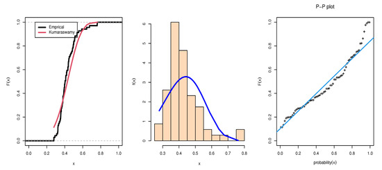
Figure 1. Plots of estimated pdfs of distributions for first Data set.

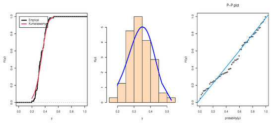
Figure 2. Plots of estimated pdfs of distributions for second Data set.

Table 5, Figure 1 and Figure 2, confirmed the fitting of the KuD to the data.

The MLE and Bayesian estimation method for stress-strength reliability model are obtain for parameters of the model based on progressive first-failure in Table 6. $k=3$ The scheme 1 is Type-II first failure where $R_1=(0^{**17},5)$ and $R_2=(0^{**17},3)$, where ${}^{**}$ point to replication of censored scheme.

Table 6. MLE and Bayesian estimation method for stress-strength reliability.

		MLE			Bayesian
Scheme		Estimates	SE	R	Estimates	SE	R
Complelet	${\alpha }_1$	3.9891	0.3556	0.7344	4.0046	0.3115	0.7418
	${\lambda }_1$	19.7760	5.2003		20.3114	4.6123
	${\alpha }_2$	5.1278	0.4444		5.3213	0.4118
	${\lambda }_2$	169.5333	71.7588		218.8506	68.1867
1	${\alpha }_1$	6.3335	1.2231	0.7487	5.9833	0.7817	0.7723
	${\lambda }_1$	59.9327	61.2251		49.1219	29.0219
	${\alpha }_2$	5.6170	0.9304		5.7488	0.7462
	${\lambda }_2$	100.6982	94.3161		137.1196	87.5453
2	${\alpha }_1$	4.5667	0.7452	0.7802	4.7140	0.5886	0.8055
	${\lambda }_1$	10.8924	6.1630		12.8144	5.4122
	${\alpha }_2$	5.1437	0.6808		5.4287	0.6144
	${\lambda }_2$	60.6901	39.9974		95.0598	31.6362

x1 is 0.279, 0.309, 0.324, 0.332, 0.351, 0.356, 0.361, 0.373, 0.380, 0.389, 0.394, 0.402, 0.411, 0.420, 0.435, 0.441, 0.450, 0.477. x2 is 0.199, 0.248, 0.257, 0.276, 0.283, 0.291, 0.299, 0.306, 0.309, 0.318, 0.330, 0.340, 0.343, 0.365, 0.381, 0.383, 0.396, 0.404.

The scheme 2 is Progressive first failure where $R_1=(5,0^{**17})$ and $R_2=(3,0^{**17})$. x1 is 0.279, 0.324, 0.332, 0.351, 0.373, 0.380, 0.389, 0.394, 0.402, 0.411, 0.420, 0.435, 0.441, 0.450, 0.477, 0.493, 0.501, 0.514. x2 is 0.199, 0.248, 0.257, 0.276, 0.283, 0.291, 0.299, 0.306, 0.309, 0.318, 0.330, 0.343, 0.365, 0.381, 0.383, 0.396, 0.417, 0.426.

Table 6 show Bayesian estimation is the best estimation method according to SE and reliability. Furthermore, we show scheme 2 has the reliability of 0.7803 for ML and 0.8055 for Bayesian which is a better scheme than other schemes. Figure 3 and Figure 4 show convergence plots of MCMC for parameter estimates of KuD for different schemes.

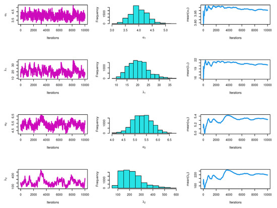
Figure 3. Convergence plots of MCMC for parameter estimates of this model when complete sample.

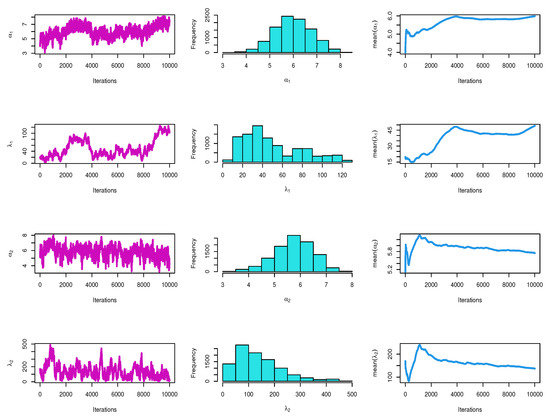
Figure 4. Convergence plots of MCMC for parameter estimates of this model when scheme 1.

6. Conclusions

In this article, we have considered estimation of the reliability R when the observed data are progressive first failure censored coming from KuD distribution. For comparing the results obtained using various methods, we have obtained the MSEs for the reliability R. In the case of Bayesian estimation, looking at the limitation of Lindley estimation to point and interval estimation, we perform the approximation using the MCMC technique also. For different censoring schemes, for comparison of point estimates, we list the MSEs from the ML and Bayesian methods in Table 1 and Table 2. Further, for interval estimation, comparison criteria are set as the interval length and coverage probability of the estimates and are tabulated in Table 3 and Table 4. The performance of the unknown parameters ${\alpha }_1$, ${\lambda }_1$, ${\alpha }_2$, and ${\lambda }_2$ and the system of stress-strength reliability in practical applications were demonstrated using two real data sets. The goodness of fit of the methods estimators for each real data set was examined using the KS, and the results were sufficient and satisfactory. The balanced loss functions give an efficient Bayesian estimator, as shown by the experimental findings. The ML estimates are compared by Bayesian estimates which seem to be better. For the Bayesian estimates, when two approximation methods namely Lindley and MCMC methods are compared, the performance of the two methods are quite close in terms of estimated MSEs.

References

- Weerahandi, S.; Johnson, R.A. Testing reliability in a stress-strength model when X and Y are normally distributed. Technometrics 1992, 34, 83–91. [Google Scholar] [CrossRef]
- Surles, J.G.; Padgett, W.J. Inference for reliability and stress-strength for a scaled Burr Type X distribution. Lifetime Data Anal. 2001, 7, 187–200. [Google Scholar] [CrossRef]
- Al-Mutairi, D.K.; Ghitany, M.E.; Kundu, D. Inferences on stress-strength reliability from Lindley distributions. Commun. Stat.-Theory Methods 2013, 42, 1443–1463. [Google Scholar] [CrossRef]
- Rao, G.S.; Aslam, M.; Kundu, D. Burr-XII distribution parametric estimation and estimation of reliability of multicomponent stress-strength. Commun. Stat.-Theory Methods 2015, 44, 4953–4961. [Google Scholar] [CrossRef]
- Singh, S.K.; Singh, U.; Yaday, A.; Viswkarma, P.K. On the estimation of stress strength reliability parameter of inverted exponential distribution. Int. J. Sci. World 2015, 3, 98–112. [Google Scholar] [CrossRef][Green Version]
- Almetwally, E.M.; Almongy, H.M. Parameter estimation and stress-strength model of Power Lomax distribution: Classical methods and Bayesian estimation. J. Data Sci. 2020, 18, 718–738. [Google Scholar] [CrossRef]
- Alshenawy, R.; Sabry, M.A.; Almetwally, E.M.; Almongy, H.M. Product Spacing of Stress–Strength under Progressive Hybrid Censored for Exponentiated-Gumbel Distribution. Comput. Mater. Contin. 2021, 66, 2973–2995. [Google Scholar] [CrossRef]
- Alamri, O.A.; Abd El-Raouf, M.M.; Ismail, E.A.; Almaspoor, Z.; Alsaedi, B.S.; Khosa, S.K.; Yusuf, M. Estimate stress-strength reliability model using Rayleigh and half-normal distribution. Comput. Intell. Neurosci. 2021, 2021. [Google Scholar] [CrossRef] [PubMed]
- Sabry, M.A.; Almetwally, E.M.; Alamri, O.A.; Yusuf, M.; Almongy, H.M.; Eldeeb, A.S. Inference of fuzzy reliability model for inverse Rayleigh distribution. AIMS Math. 2021, 6, 9770–9785. [Google Scholar] [CrossRef]
- Abu El Azm, W.S.; Almetwally, E.M.; Alghamdi, A.S.; Aljohani, H.M.; Muse, A.H.; Abo-Kasem, O.E. Stress-Strength Reliability for Exponentiated Inverted Weibull Distribution with Application on Breaking of Jute Fiber and Carbon Fibers. Comput. Intell. Neurosci. 2021, 2021. [Google Scholar] [CrossRef]
- Okabe, T.; Otsuka, Y. Proposal of a Validation Method of Failure Mode Analyses based on the Stress-Strength Model with a Support Vector Machine. Reliab. Eng. Syst. Saf. 2021, 205, 107247. [Google Scholar] [CrossRef]
- Bhattacharyya, G.K.; Johnson, R.A. Estimation of reliability in a multicomponent stress-strength model. J. Am. Stat. Assoc. 1974, 69, 966–970. [Google Scholar] [CrossRef]
- Kotb, M.S.; Raqab, M.Z. Estimation of reliability for multi-component stress–strength model based on modified Weibull distribution. Stat. Pap. 2020, 2020, 1–35. [Google Scholar] [CrossRef]
- Maurya, R.K.; Tripathi, Y.M. Reliability estimation in a multicomponent stress-strength model for Burr XII distribution under progressive censoring. Braz. J. Probab. Stat. 2020, 34, 345–369. [Google Scholar] [CrossRef]
- Mahto, A.K.; Tripathi, Y.M.; Kızılaslan, F. Estimation of Reliability in a Multicomponent Stress–Strength Model for a General Class of Inverted Exponentiated Distributions Under Progressive Censoring. J. Stat. Theory Pract. 2020, 14, 1–35. [Google Scholar] [CrossRef]
- Mahto, A.K.; Tripathi, Y.M. Estimation of reliability in a multicomponent stress-strength model for inverted exponentiated Rayleigh distribution under progressive censoring. OPSEARCH 2020, 57, 1043–1069. [Google Scholar] [CrossRef]
- Wang, L.; Dey, S.; Tripathi, Y.M.; Wu, S.J. Reliability inference for a multicomponent stress–strength model based on Kumaraswamy distribution. J. Comput. Appl. Math. 2020, 376, 112823. [Google Scholar] [CrossRef]
- Wang, L.; Wu, K.; Tripathi, Y.M.; Lodhi, C. Reliability analysis of multicomponent stress–strength reliability from a bathtub-shaped distribution. J. Appl. Stat. 2020, 1–21. [Google Scholar] [CrossRef]
- Jha, M.K.; Dey, S.; Alotaibi, R.M.; Tripathi, Y.M. Reliability estimation of a multicomponent stress-strength model for unit Gompertz distribution under progressive Type II censoring. Qual. Reliab. Eng. Int. 2020, 36, 965–987. [Google Scholar] [CrossRef]
- Rasekhi, M.; Saber, M.M.; Yousof, H.M. Bayesian and classical inference of reliability in multicomponent stress-strength under the generalized logistic model. Commun. Stat.-Theory Methods 2020, 1–12. [Google Scholar] [CrossRef]
- Alotaibi, R.M.; Tripathi, Y.M.; Dey, S.; Rezk, H.R. Bayesian and non-Bayesian reliability estimation of multicomponent stress–strength model for unit Weibull distribution. J. Taibah Univ. Sci. 2020, 14, 1164–1181. [Google Scholar] [CrossRef]
- Maurya, R.K.; Tripathi, Y.M.; Kayal, T. Reliability Estimation in a Multicomponent Stress-Strength Model Based on Inverse Weibull Distribution. Sankhya B 2021, 1–38. [Google Scholar] [CrossRef]
- Kohansal, A.; Shoaee, S. Bayesian and classical estimation of reliability in a multicomponent stress-strength model under adaptive hybrid progressive censored data. Stat. Pap. 2021, 62, 309–359. [Google Scholar] [CrossRef]
- Jana, N.; Bera, S. Interval estimation of multicomponent stress–strength reliability based on inverse Weibull distribution. Math. Comput. Simul. 2022, 191, 95–119. [Google Scholar] [CrossRef]
- Chandra, S.; Owen, D.B. On estimating the reliability of a component subject to several different stresses (strengths). Nav. Res. Logist. Quart. 1975, 22, 31–39. [Google Scholar] [CrossRef]
- Hlawka, P. Estimation of the Parameter p = P(X < Y < Z); No.11, Ser. Stud. i Materiaty No. 10 Problemy Rachunku Prawdopodobienstwa; Prace Nauk. Inst. Mat. Politechn.: Wroclaw, Poland, 1975; pp. 55–65. (In Polish) [Google Scholar]
- Singh, N. On the estimation of Pr(X1 < Y < X2). Commun. Statist. Theory Meth. 1980, 9, 1551–1561. [Google Scholar]
- Dutta, K.; Sriwastav, G.L. An n-standby system with P(X < Y < Z). IAPQR Trans. 1986, 12, 95–97. [Google Scholar]
- Ivshin, V.V. On the estimation of the probabilities of a double linear inequality in the case of uniform and two-parameter exponential distributions. J. Math. Sci. 1998, 88, 819–827. [Google Scholar] [CrossRef]
- Hanagal, D.D. Estimation of system reliability in multicomponent series stress—strength model. J. Indian Statist. Assoc. 2003, 41, 1–7. [Google Scholar]
- Waegeman, W.; De Baets, B.; Boullart, L. On the scalability of ordered multi-class ROC analysis. Comput. Statist. Data Anal. 2008, 52, 33–71. [Google Scholar] [CrossRef]
- Chumchum, D.; Munindra, B.; Jonali, G. Cascade System with Pr(X < Y < Z). J. Inform. Math. Sci. 2013, 5, 37–47. [Google Scholar]
- Pan, G.; Wang, X.; Zhou, W. Nonparametric statistical inference for P(X < Y < Z). Indian J. Stat. 2013, 75, 118–138. [Google Scholar]
- Patowary, A.N.; Sriwastav, G.L.; Hazarika, J. Inference of R = P(X < Y < Z) for n-Standby System: A Monte-Carlo Simulation Approach. J. Math. 2016, 12, 18–22. [Google Scholar]
- Saini, S.; Tomer, S.; Garg, R. On the reliability estimation of multicomponent stress–strength model for Burr XII distribution using progressively first-failure censored samples. J. Stat. Comput. Simul. 2021, 1–38. [Google Scholar] [CrossRef]
- Kohansal, A.; Fernández, A.J.; Pérez-González, C.J. Multi-component stress–strength parameter estimation of a non-identical-component strengths system under the adaptive hybrid progressive censoring samples. Statistics 2021, 1–38. [Google Scholar] [CrossRef]
- Hassan, M.K. On Estimating Standby Redundancy System in a MSS Model with GLFRD Based on Progressive Type II Censoring Data. Reliab. Theory Appl. 2021, 16, 206–219. [Google Scholar]
- Wu, S.J.; Kus, C. On estimation based on progressive first-failure-censored sampling. Comput. Stat. Data Anal. 2009, 53, 3659–3670. [Google Scholar] [CrossRef]
- Balakrishnan, N.; Aggarwala, R. Progressive Censoring: Theory, Methods, and Applications; Springer Science & Business Media Birkhauser Boston: Cambridge, MA, USA, 2000. [Google Scholar]
- Kumaraswamy, P. A generalized probability density function for double-bounded random processes. J. Hydrol. 1980, 46, 79–88. [Google Scholar] [CrossRef]
- Jones, M.C. Kumaraswamy’s distribution: A beta-type distribution with some tractability advantages. J. Statist. Methodol. 2009, 6, 70–81. [Google Scholar] [CrossRef]
- Golizadeh, A.; Sherazi, M.A.; Moslamanzadeh, S. Classical and Bayesian estimation on Kumaraswamy distribution using grouped and ungrouped data under difference of loss functions. J. Appl. Sci. 2011, 11, 2154–2162. [Google Scholar] [CrossRef]
- Sindhu, T.N.; Feroze, N.; Aslam, M. Bayesian analysis of the Kumaraswamy distribution under failure censoring sampling scheme. Int. J. Adv. Sci. Technol. 2013, 51, 39–58. [Google Scholar]
- Sharaf EL-Deen, M.M.; AL-Dayian, G.R.; EL-Helbawy, A.A. Statistical inference for Kumaraswamy distribution based on generalized order statistics with applications. J. Adv. Math. Comput. Sci. 2014, 4, 1710–1743. [Google Scholar]
- Wang, L. Inference for the Kumaraswamy distribution under -record values. J. Comput. Appl. Math. 2017, 321, 246–260. [Google Scholar] [CrossRef]
- Kumar, M.; Singh, S.K.; Singh, U.; Pathak, A. Empirical Bayes estimator of parameter, reliability and hazard rate for Kumaraswamy distribution. Life Cycle Reliab. Saf. Eng. 2019, 8, 243–256. [Google Scholar] [CrossRef]
- Fawzy, M.A. Prediction of Kumaraswamy distribution in constant-stress model based on type-I hybrid censored data. Stat. Anal. Data Min. ASA Data Sci. J. 2020, 13, 205–215. [Google Scholar] [CrossRef]
- Ferguson, T. A Course in Large Sample Theory. In Chapman & Hall Texts in Statistical Science Series; Taylor & Francis: Milton Park, VA, USA, 1996. [Google Scholar]
- Efron, B. The Jackknife, the Bootstrap and other Resampling Plans. In CBMS-NSF Regional Conference Series in Applied Mathematics; SIAM: Philadelphia, PA, USA, 1982; Volume 38. [Google Scholar]
- Hall, P. Theoretical comparison of bootstrap confidence intervals. Ann. Stat. 1988, 16, 927–953. [Google Scholar] [CrossRef]
- Zellner, A. Bayesian and non-Bayesian estimation using balanced loss functions. In Statistical Decision Theory and Methods; Berger, J.O., Gupta, S.S., Eds.; Springer: New York, NY, USA, 1994; pp. 337–390. [Google Scholar]
- Ahmadi, J.; Jozani, M.J.; Marchand, E.; Parsian, A. Bayes estimation based on k- record data from a general class of distributions under balanced Type loss functions. J. Stat. Plan. Inference 2009, 139, 1180–1189. [Google Scholar] [CrossRef]
- Lindley, D.V. Approximate Bayesian method. Trab. Estad. 1980, 31, 223–237. [Google Scholar] [CrossRef]
- Chen, M.H.; Shao, Q.M. Monte Carlo estimation of Bayesian credible and HPD intervals. J. Comput. Graph. Stat. 1999, 8, 69–92. [Google Scholar]
- Balakrishnan, N.; Sandhu, R.A. A simple simulational algorithm for generating progressive Type-II censored samples. Am. Stat. 1995, 49, 229–230. [Google Scholar]
- Kundu, D.; Gupta, R.D. Estimation of P[Y < X] for Weibull distributions. IEEE Trans. Reliab. 2016, 55, 270–280. [Google Scholar]
Publisher’s Note: MDPI stays neutral with regard to jurisdictional claims in published maps and institutional affiliations. |
© 2021 by the authors. Licensee MDPI, Basel, Switzerland. This article is an open access article distributed under the terms and conditions of the Creative Commons Attribution (CC BY) license (https://creativecommons.org/licenses/by/4.0/).