Abstract
Recent advances in experimental biology studies have produced large amount of molecular activity data. In particular, individual patient data provide non-time series information for the molecular activities in disease conditions. The challenge is how to design effective algorithms to infer regulatory networks using the individual patient datasets and consequently address the issue of network symmetry. This work is aimed at developing an efficient pipeline to reverse-engineer regulatory networks based on the individual patient proteomic data. The first step uses the SCOUT algorithm to infer the pseudo-time trajectory of individual patients. Then the path-consistent method with part mutual information is used to construct a static network that contains the potential protein interactions. To address the issue of network symmetry in terms of undirected symmetric network, a dynamic model of ordinary differential equations is used to further remove false interactions to derive asymmetric networks. In this work a dataset from triple-negative breast cancer patients is used to develop a protein-protein interaction network with 15 proteins.
1. Introduction
Recent advances in experimental biology studies have produced large amount of molecular activity data [1]. In particular, the single-cell experiments are able to quantify gene expression activities or protein abundances in a large number of single cells in a single experiment, which provides rich information to study the cellular heterogeneity [2]. A similar datum type is the individual patient data that measure the cellular information from the cell lines of each patients [3]. An important question is how to analyse the individual patient datasets and derive biological information from the datasets [4]. A further related question is how to reconstruct gene/protein connection networks and address the issue of directed regulations in the developed asymmetric networks [5,6,7,8].
The inference methods for constructing regulatory networks can be mainly classified into three major types, namely the correlation-based methods, dynamic model methods and machine learning methods [9,10,11]. The correlation-based methods use one or more statistical qualities to measure the relationship between pairs of variables in a network. Several statistical measure have been used to calculate the distances between the variables using the omics datasets [12,13,14]. The correlation-based methods have also been used to find the connections between various types of molecules in cells [15,16,17]. An alternative approach is mutual information, which can measure the nonlinear relationships between pairs of variables [18]. In addition, the regression-based methods are able to establish the systematic regulations between all the variables in the system [19]. LASSO and ridge regression are two major techniques used in the regression-based methods to construct sparse system models [19,20]. A broader category of these methods is called the causal network methods that also contain the Bayesian network methods and path-consistency methods [21,22]. The path-consistency algorithms have been designed by the combination of mutual information, conditional mutual information or part mutual information [23,24,25]. Due to the computing efficiency, the correlation-based methods are able to develop large-scale regulatory network models.
The widely used dynamic models are based on differential equation systems that describe the detailed dynamics of regulatory networks and make testable predictions [26,27,28,29]. Due to the computing time for simulating models, the differential equation models normally are limited to small-scale systems. Another issue in dynamic modelling is the inference of model parameters. If the network model is large, the parameter space is complex and it is difficult to deal with a large number of unknown parameters of the model [30]. To address this issue, it is proposed to use the hybrid-methods that combine the statistical methods to design a static model and the differential equation methods for a dynamic model together [31,32,33]. In recent years, machine learning algorithms have been used to infer regulatory networks using omics datasets and single-cell data [34,35,36,37].
Since the Monocle algorithm was first proposed to infer the pseudo-time trajectories of single cells [38], several methods were developed to determine the positions of single cells during the cellular processes. The algorithms for constructing pseudo-time trajectories normally have two major steps. The first step reduces the dimension of the dataset for visualisation and the second step builds the trajectories based on the low-dimensional dataset. Several algorithms use the minimum-spanning tree (MST) or shortest path to build the major structure of the trajectory. Then each cell will be projected to the major structure to form the trajectory in the second step [39,40]. In recent years, manifold learning has also been used for pseudo-time inference of single-cell data [41]. Diffusion map has been used to explore the developmental continuum of cell-fate transitions [42]. A recent comparison study have tested the effectiveness and efficiency of several major algorithms [43]. In addition, several pipelines have been developed for reconstructing the genetic regulatory networks using single-cell data [32,44,45]
Individual patient data are collections of raw data from several patients with a certain disease [3]. Although substantial studies have been conducted for the statistical analysis of the individual patient data, limited attempts have been conducted so far to reconstruct regulatory networks using this type of datasets. In this work we propose a general pipeline to use individual patient data to infer protein-protein interaction networks. We first select several important proteins in an individual patient dataset and use a statistical package to interpolate the missing values. Then we use the SCOUT algorithm to construct the pseudo-time trajectory of individual patients. The Gaussian process regression method is used to smooth the expression data. The path-consistency algorithm is applied to infer the structure of protein-protein interaction network. To obtain the model dynamics, the ordinary differential equation model was used to remove the false regulations from the static network.
2. Materials and Methods
2.1. Experimental Data
Breast cancer is one of the most common types of life-threatening disease in females worldwide [46]. Although more than 80 percent of breast cancers can be treated by targeted therapies, triple-negative breast cancer (TNBC) is an important unmet clinical problem. Recently, Lawrence et al. conducted a deep proteomic characterisation of TNBC cell lines and tissues using mass spectrometry [47]. This individual patient dataset includes 40 breast cancer lines and four primary breast tumour cell lines, resulting in peptides of around 12,000 distinct proteins. Among them, at least 9000 proteins have been found in each cell line [47]. In this study, we use this dataset to infer the protein-protein interaction network. To generate a manageable sample size, we concentrate on proteins from cell signalling pathways whose functions are connected to cell proliferation. The mitogen-activated protein (MAP) kinase pathway is an important pathway to control cell proliferation. This pathway includes three parallel pathways, namely the ERK pathway, JNK pathway and p38 pathway [48]. The pathway maps from Kyoto Encyclopedia of Genes and Genomes (KEGG) is employed as the reference for selecting proteins [49].
2.2. Static Network Development
Let X be a random variable with density function . Entropy in statistical mechanics is a measure of thermal energy per unit temperature that is unavailable for doing useful work in a system, defined by.
for the discrete random variables. Here are samples of random variable X. In addition, the joint entropy of two discrete random variables X and Y, which have joint density function , is defined by
where are samples of random variable Y.
Mutual information is an alternative approach to measure the relationship of two random variables. Compared with the correlation coefficient, this method is able to measures the nonlinear relationship of two random variables. Consider random variables with marginal density functions and for X and Y, respectively. We can calculate mutual information using
Alternatively, the entropies of X, Y and can also be used to calculate mutual information using
Unlike correlation coefficient, two random variables are independent of each other if the mutual information value is zero [23]. Since the value of mutual information is non-negative, a larger value of mutual information normally means these two random variables have closer relationship.
When a system contains more random variables, we can calculate the mutual information of each pair of random variables for measuring the relationship. In this case, a large value of mutual information may not be the indicator of close relationship. For example, random variables X and Y as well as Y and Z have close relationship, which may lead to a large value of mutual information between X and Z that actually have not close relationship. To avoid such false relationship, conditional mutual information is defined for the conditional relationship of two random variables X and Y in the presence of the third variable Z, given by
where is defined as the joint entropy of these three random variables. Based on the joint density function of these three random variables, the joint entropy is defined by
where , and are samples of random variables X, Y and Z, respectively.
Although mutual information may lead to false close relationship, the problem of the conditional mutual information is that this measure may underestimate the relationship of two random variable, which may ignore the true relationship between random variables. To solve this problem, part mutual information is proposed to measure the relationship of two random variables X and Y in the presence of the third random variable Z [25]. We first give the definition of partial independence of the random variables, given by
where
Based on the partial independence (7), the definition of part mutual information is given by
where is the marginal density function of Z.
The path-consistency algorithm is used to develop a static network using the threshold method. Instead of selecting edges that have larger correlation measures, this algorithm remove edges whose correlation measure values are smaller than the threshold value. The threshold value is determined based on the required sparsity of the developed network. In this work, both the MI values and higher order PMI are used to remove edges. If the MI values are used only, the developed network is termed of zero-order PMI network. Based on two proteins that are adjacent in the zero-order network, we then find stock k that is connected to both proteins i and j. If this protein k does not exist, no first-order PMI exists for edge that connects proteins i and j, and this edge remains in the first-order PMI network. If one or more proteins exist, we need to calculate the first order PMI values and then determine whether to remove edge if all PMI values are less then the threshold value or keep that edge if one of the PMI values is larger than the threshold value. A similar procedure is applied to higher order PMI values. The detailed process of the path-consistency algorithm can be found in reference [23].
2.3. Data Processing
To reconstruct a dynamic network, the individual patient data need to be transformed into time series data. In this work we use our recently proposed SCOUT algorithm for the pseudo-time ordering of individual patient data to find the pseudo-ordering of patients [40]. This algorithm includes two major steps. In the first step, the modified local linear embedding method is applied for dimensional reduction, which project each cell in the high-dimensional space into a low-dimensional embedding space for data visualisation. The second step infers the trajectory based on the low dimensional dataset. We first use the Gaussian mixture model to find the landmarks based on the densities of individual patients in the low-dimensional space. Then MST is developed that connects all landmarks. To reduce the uncertainties in the MST, we use 15 landmarks for this dataset. We also determine the starting landmark based on the distances between these landmarks. This MST determines the structure of the inferred trajectory. We then project each cell to a point on the edge of the MST. We use the Apollonian score to determine the relative positions of each patient.
The activities of each protein in the inferred pseudo-time trajectory is quite noisy and it is difficult to simulate these experimental data using mathematical model directly. Thus, in the next step, the Gaussian process regression method is used to smooth the pseudo-time data. Assume that protein i has activities , and the activity can be represented by the Gaussian noise model
where is the non-polynomial smoothing result representing underlying expression value of protein i at time t, and is the irreducible noises.
2.4. Mathematical Modelling
We recently proposed a mathematical model to simulate the protein activities based on the omics dataset [31]. For a network with N proteins, the kinase activities of the i-th protein are denoted as at time t. Generally, for a regulatory network, the dynamic protein activities is modelled by the following differential equations
where is model parameters, is the degradation rate. The regulatory function represents positive and/or negative regulations from other proteins to protein i. The key issue is how to design this regulatory function. Instead of using the summation of positive and negative regulatory functions in our previous study [33], this work proposes to use the following regulatory function
where , and will be estimated by matching the experimental data using the approximate Bayesian computation (ABC) method. If and , protein j positively regulates protein i; if and , protein j negatively regulates protein i; if and , protein j has no regulatory relationship with protein i. Since it is rare to generate a sample with value of exact zero, we use the following indicator function, defined by
where is a sample generated from the uniformly distributed random variable . Thus, for a network with N proteins, the number of the unknown parameters is , namely , , and . Using the static network derived from the path-consistency algorithm, the number of unknown parameters can be reduced substantially.
The absolute error is used to quantify the error between the simulated protein activities and experimental data, given by
where and are the simulated data and observation data of protein i at time point j, respectively.
2.5. Robustness Analysis
Since we can obtain different estimates of model parameters in different implementations of the ABC algorithm, we use the robustness property as an additional criterion to select the estimated model parameters. We used the definition by Kitano [50] to quantify the robustness of a network model. For the given model parameter , we consider a set of perturbations P. For each perturbation, we simulate the model and derive the simulation which is called the perturbed system over the perturbation. The average simulation is measured by
where is the probability of perturbation p. If perturbations have the same probability, it is the average of all the perturbed simulations. Thus, the average behaviour (AB) is defined by
where is the unperturbed simulation using the estimated parameters at time point j. Please note that is a vector of all variables. In addition, we define the nominal behaviour (NB) as
For each rate constant , the perturbation is set to with a Gaussian distribution. Here is the perturbation strength and the value of is determined by simulations. For each set of estimate, we generate 1000 sets of perturbed parameters. The system with a particular set of estimate is more robust if the difference between the perturbed 1000 simulations and unperturbed simulation is smaller.
3. Results
3.1. Pseudo-Time Trajectory Inference
Based on the Uniprot Entry of each gene, we first find the corresponding proteins in the TNBC proteome excel which represents intensity-based absolute protein abundance (iBAQ) profile of each sample. We initially select 60 important proteins from the MAP kinase pathway from the 1200 proteins sampled in the database showing large variations [47]. We also include the upstream protein PCK and the down-stream transcriptional factor MSK1/2. In addition, AKT is also included for testing the cross-talk between the MAP kinase pathway and Akt-PI3K pathway. For these 60 proteins, there are quite several missing values because of experimental conditions. There are 30 proteins that have more than 50% missing values. Thus, we choose 27 proteins that have more than 50% observation values.
For these 27 proteins, we use an R package missMDA [51] which use the principal component methods to deal with incomplete data sets. For this dataset, we use the regularised iterative PCA algorithm. First, the means of the variables change after each imputation. Next, the algorithm use cross-validation to tune the number of dimensions as a priori. We implement leave-one-out, k-fold and generalised cross-validation to obtain the dimension that minimises the mean square error of prediction. Finally, we choose the imputed matrix which falls a predefined threshold. Finally, we selected 15 proteins by excluding a few protein isoforms and proteins whose smoothed data still have large variations. These 15 proetins are PKC, Ras, Raf1, RafB, MEK1, MKK3, MKK4, MKK6, ERK, P38, JNK, MSK1/2, Akt, TAB, and DAXX.
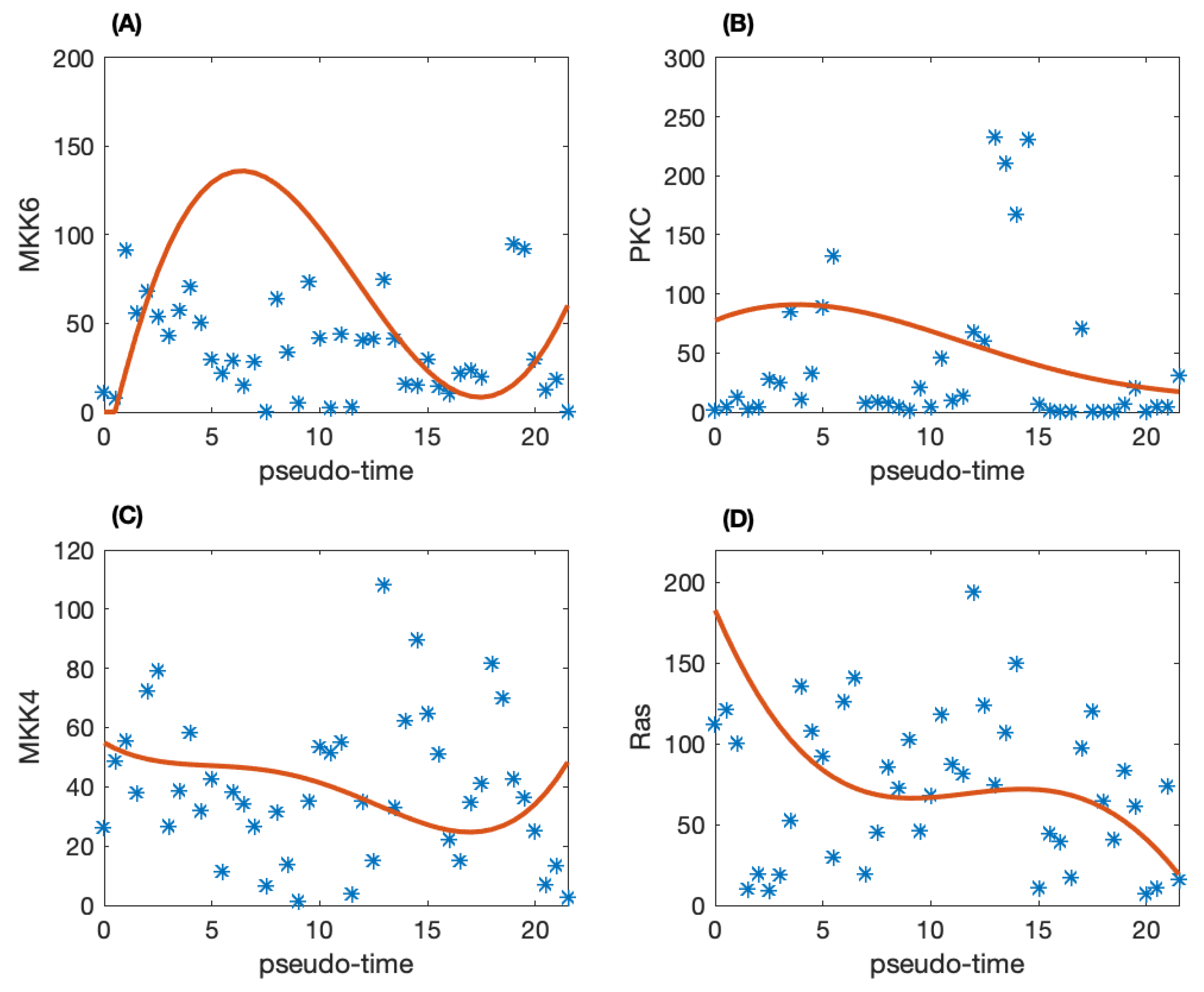
To construct dynamic network, the pseudo-trajectory is inferred for the time dependent model. We use the SCOUT algorithm to infer the pseudo-time trajectory of the individual patients to obtain the developmental process of TNBC. Figure 1 shows the raw data for the pseudo-time trajectory of four proteins. It is clear that there is much noise in the raw pseudo-time trajectory. Thus, the Gaussian process regression method is employed to remove the noise in the data. The solid-line in Figure 1 is the smoothed protein activity data. Compared with the raw data shown as star in Figure 1, the smoothed data can be used for mathematical modeling.
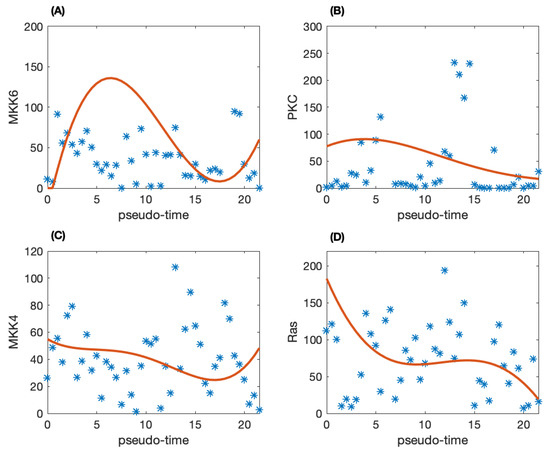
Figure 1.
The pseudo-time trajectory of four proteins and the corresponding smoothed proteomic data. (A) Protein MKK6; (B) PKC; (C) MKK4; (D) Ras.
3.2. Static Networks Construction
After the selection of 15 proteins, we use the Path-consistency algorithm using PMI to reconstruct the static regulatory network. Since the network density is determined by the threshold value, we use the algorithm with different threshold values to obtain networks with different number of edges. Our experience in gene network construction shows that, when the number of edges is relatively small, several regulations are not included in the developed static network. Thus, we use a relatively small threshold values to select the top undirected 50 edges. Since one edge represents two directed regulations, the total potential regulations in the developed network is 100.
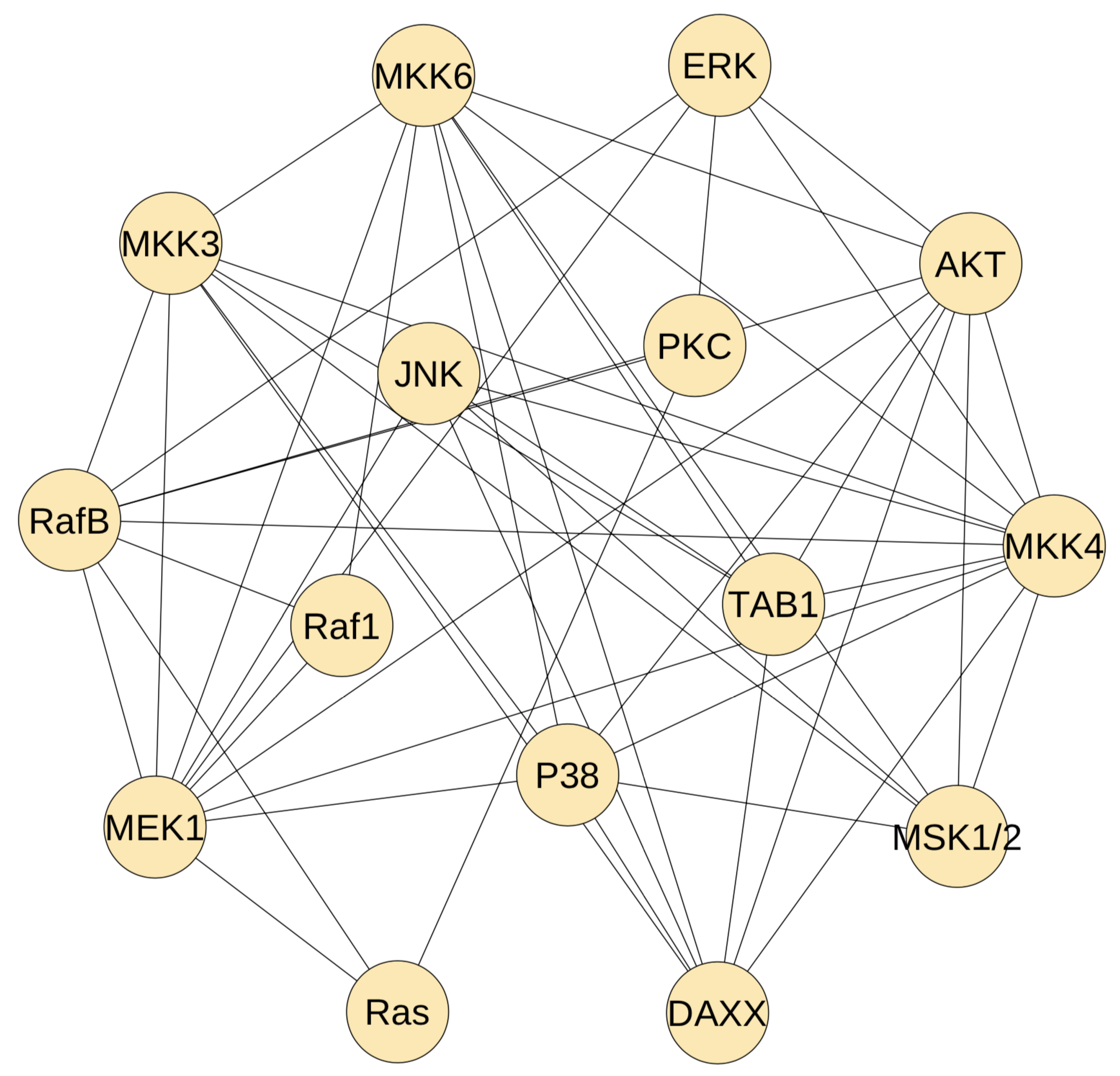
Figure 2 gives the developed static network. Each protein on average has 6.7 edges to connect the other proteins. It shows that the proteins in the upstream pathway has less connections. For example, Ras protein has only three connections, and a similar observation is applied to protein Raf1. However, the MAP kinase kinase proteins have much more regulations. For example, MEK1 has 10 connections and MKK4 has 11 regulations. These observations are consistent with the regulation complexity of the MAP kinase signalling pathway, namely there are more cross-talk in the MAP kinase modules. However, the selected regulations in Figure 2 are much more than the real regulations in the MAP kinase pathway. We need to use the dynamic model to delete false regulations from the developed static network.
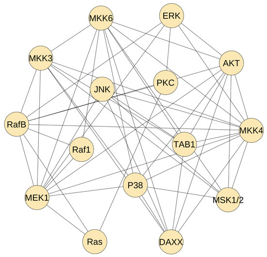
Figure 2.
The inferred static network using the path-consistency algorithm with PMI. This network has 15 proteins in the MAP kinase pathway and 50 mutual regulations.
3.3. Inference of Model Parameters
Based on the static network in Figure 2 with 15 proteins and 50 mutual regulations, we first use the Approximate Bayesian Computation (ABC) rejection method to estimate the unknown model parameters. Since the protein activities of different proteins have large variations, we normalise the activities of protein i using
where are the smoothed protein activities at time j. In this way, we can compare the coefficient values under the same condition. That is also why the absolute error (12) is used to quantify the simulation error. Instead of simulating the model in the whole time period using one initial condition at , we use the smoothed protein activities at time point as the initial condition to simulate the model in the time period , and then calculate the simulation error at [52]. For model parameters , and , it is assumed that the prior distribution follows the uniform distribution in the interval . We test the different values of B for achieving better accuracy of the simulations. The final value used in the simulation is .
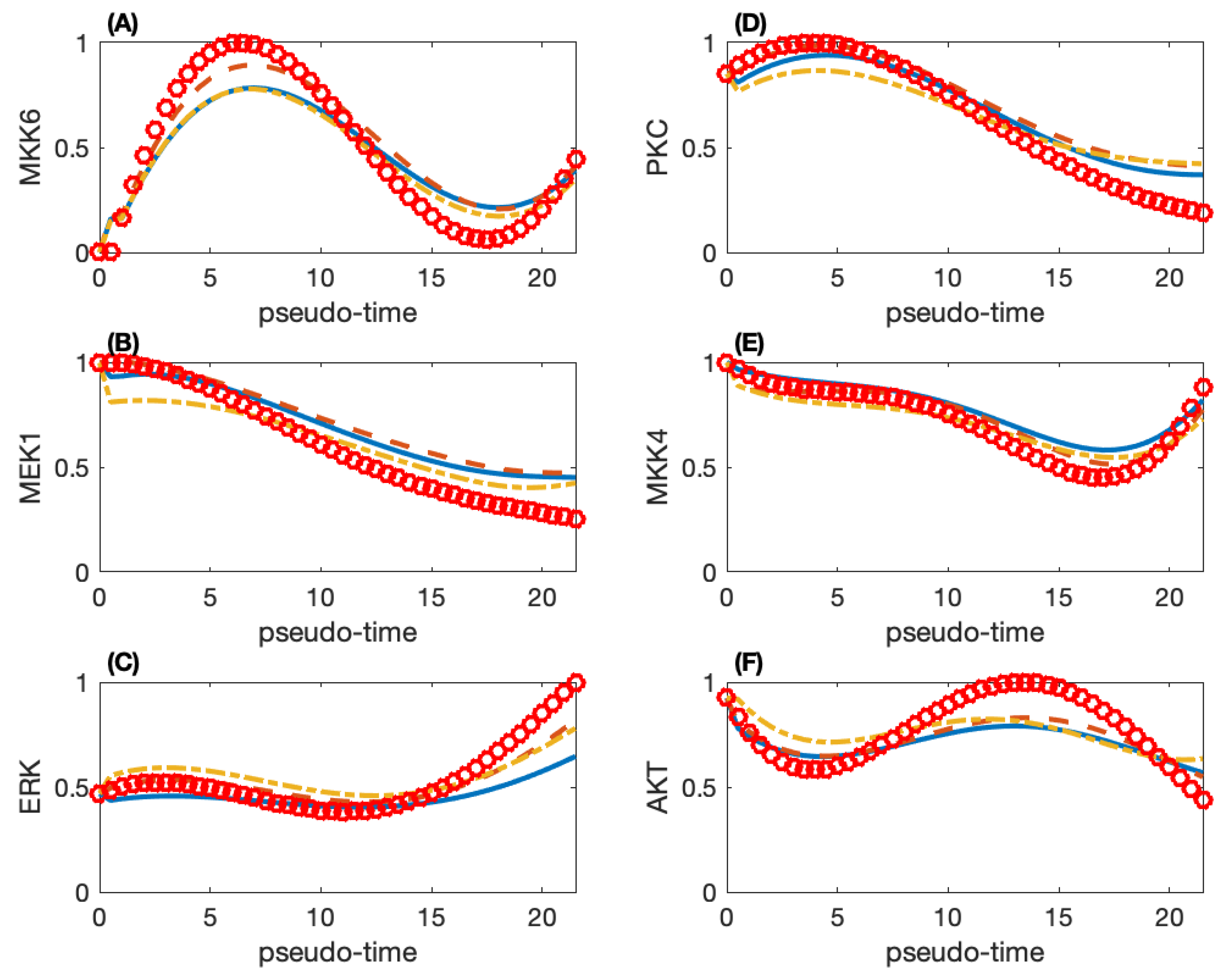
We use the ABC rejection algorithm to obtain 10,000 sets of parameter estimates and select the top 100 sets with smaller simulation errors for further analysis. We calculate the model robustness using the top 10 sets of parameters and determine the final set from these 10 sets based on the robustness property. Figure 3 gives the simulated and smoothed observed protein activities of six proteins. These six proteins have different trends in protein activities. The other proteins have a trend that is close to one of the patterns in Figure 3. For example, MKK3 has a quite close trend to that of MKK6 in Figure 3A, and RafB has similar protein activities as those ERK in Figure 3C. However, AKT in Figure 3F has a unique pattern, and whose activities reach the peak at , possibly because AKT is not a protein in the MAP kinase pathway.
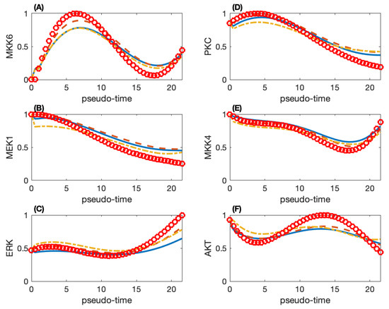
Figure 3.
Simulated protein activities and smoothed experimental data of six proteins in the MAP kinase pathway. (A) Protein MKK6; (B) MEK1; (C) ERK; (D) PKC; (E) MKK4; (F) AKT. (Red circle: smoothed observation data; solid-line: simulation of the network with 100 directed regulations; dash-line: simulation of the network with 70 directed regulations; dash-dot line: simulation of the network with 35 directed regulations.
3.4. Inference Network with Less Regulations
The inferred network in the previous subsection has 100 directed regulations that is much larger than the regulations in the signal transduction pathway. Thus, a large number of regulations should be removed from the derived network. We next use the dynamic model (9) with function (10) to remove regulations that has less impact on the system dynamics. With such a large number of regulations in the network, the removal of one or two regulations has limited effects on the system dynamics. So we choose 15 regulations in one test initially. The key criterion for removing regulations is the value of coefficients in the estimated model parameters. Since the value of a particular parameter varies in different estimates, we use the average value of the top 100 estimates. In addition, the following factors are also considered. First, if the correlation coefficient of two proteins is large, the edge connecting these two proteins should not be considered. In addition, we try to keep a minimal number of regulations to each protein. For example, more regulations are removed for MEK1 and MKK4 but less regulations are removed for Ras initially. It is relatively easy to select the first ∼10 regulations but the difference between average coefficients of the following regulations are small. Thus, different selections of the removed edges may be tested. If the removed edges have much influence on the system dynamics, we need to test a different set of regulations.
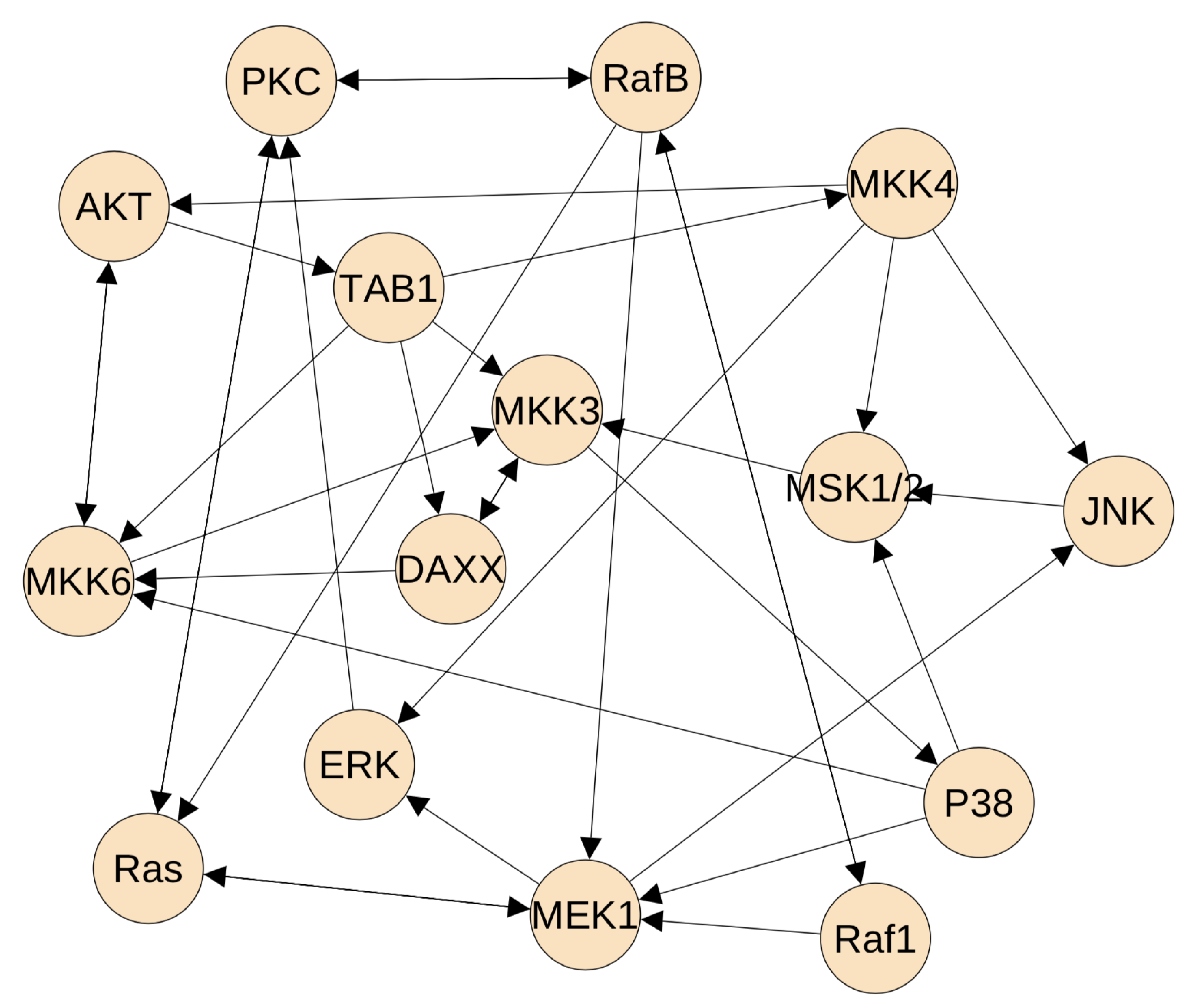
In the five removal tests in Table 1, it is relatively easy to conduct the first two tests. Only one selection is used to determine the removed edges. However, in the following tests, more selections are needed to determine the removed edges. The simulation error and the robustness property are used to determine the different selections. If the derived network has similar simulation error and robustness property as the network before removal, the selected removal is determined. In the final test (namely test 5), it is difficult to select more edges. Thus, we choose only 5 edges to be removed from the network. Figure 3 also gives the simulations of the network with 70 regulations (i.e., Test 2) and that with 35 regulations (i.e., Test 5). Figure 4 gives the final inferred network with 35 regulations.

Table 1.
Simulation error and robustness of the inferred networks in five removal tests. SE: simulation error (12); AB: average behaviour (14); NB: nominal behaviour (15). Test 0: network with 100 directed regulations without any removal; Test 1: network with 85 directed regulations; Test 2: network with 70 directed regulations; Test 3: network with 55 directed regulations; Test 4: network with 40 directed regulations; Test 5: network with 35 directed regulations.
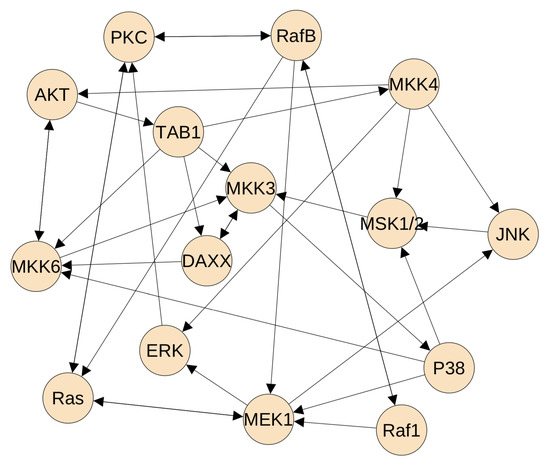
Figure 4.
The final inferred protein regulatory network of the MAP kinase pathway. This network has 35 directed regulations.
4. Conclusions
This work is aimed at designing an integrated pipeline for reconstructing protein-protein interaction networks using individual patient proteomic data. We first use the SCOUT algorithm to infer the pseudo-time trajectory for the individual patients using the proteomic data. Due to the large noise of protein abundance in the pseudo-time trajectory, we use the Gaussian process regression method to smooth the pseudo-time proteomic data. To deal with relatively large networks using dynamic models, we first use the path-consistency algorithm with part mutual information to develop a static protein-protein interaction network in order to reduce the complexity of the regulatory network. Based on the static network, we design a dynamic model of ordinary differential equations to simulate the evolution of protein activities. In this work we use develop a relatively dense static network and then remove false regulations from the developed network. Using the proteomic data of the triple negative breast cancer patients as the test problem, we develop a network model with 15 proteins in the MAP kinase pathway. Numerical results suggest that the proposed method is an effective approach to study the functions and mechanisms of relatively large regulatory networks.
Compared with our previous study [33], the developed static network in this work contains much more possible regulations. Thus, the dynamic modelling step needs to remove more false regulations. Since the removal of one or two regulations in such a large network does not have any impact on the system dynamics, we remove 15 false regulations from the network in one step mainly based on the relatively small values of the inferred model parameters. The simulation error and robustness property are used as the major criteria to remove regulations. In fact, when the regulation number in the network become smaller, it is more difficult to select false regulations. We need to test more possible cases in one test in order to ensure the reliability of the predicted network. However, this proposed framework is a manually controlled method. It would be interesting to design an integrated algorithm by qualifying the additional standard into the method.
Author Contributions
Conceptualization, T.T.; Data curation, Y.Y. and F.J.; Funding acquisition, Y.Y., F.J. and X.Z.; Investigation, Y.Y.; Methodology, X.Z., T.T.; Software, Y.Y.; Supervision, F.J.; Validation, F.J., X.Z.; Writing—original draft, T.T.; Writing—review & editing, Y.Y., F.J., X.Z., T.T. All authors have read and agreed to the published version of the manuscript.
Funding
This research was funded by National Natural Science Foundation of China (11871238, 11931019, 61773401), the Science Foundation of Wuhan Institute of Technology (20QD47), and the Foundation of Zhongnan University of Economics and Law (3173211205).
Institutional Review Board Statement
Not applicable.
Informed Consent Statement
Not applicable.
Data Availability Statement
Data sharing is not applicable to this article.
Conflicts of Interest
The authors declare no conflict of interest.
Abbreviations
The following abbreviations are used in this manuscript:
| MST | Minimum-spanning tree |
| TNBC | Triple-negative breast cancer |
| MAP | Mitogen-activated protein |
| MI | Mutual Information |
| CMI | Conditional mutual information |
| PMI | Part mutual information |
| ABC | Approximate Bayesian computation |
References
- Joyce, A.R.; Palsson, B.Ø. The model organism as a system: Integrating ‘omics’ data sets. Nat. Rev. Mol. Cell Biol. 2006, 7, 198–210. [Google Scholar] [CrossRef]
- Laehnemann, D.; Köster, J.; Szczurek, E.; McCarthy, D.J.; Hicks, S.; Robinson, M.D.; Vallejos, C.A.; Campbell, K.R.; Beerenwinkel, N.; Mahfouz, A.; et al. Eleven grand challenges in single-cell data science. Genome Biol. 2020, 21, 31. [Google Scholar] [CrossRef]
- Riley, R.D.; Lambert, P.C.; Abo-Zaid, G. Meta-analysis of individual participant data: Rationale, conduct, and reporting. BMJ 2010, 340, c221. [Google Scholar] [CrossRef] [Green Version]
- Vogel, C.; Marcotte, E.M. Insights into the regulation of protein abundance from proteomic and transcriptomic analyses. Nat. Rev. Genet. 2012, 13, 227–232. [Google Scholar] [CrossRef]
- Saint-Antoine, M.M.; Singh, A. Network inference in systems biology: Recent developments, challenges, and applications. Curr. Opin. Biotechnol. 2020, 63, 89–98. [Google Scholar] [CrossRef] [PubMed] [Green Version]
- Karlebach, G.; Shamir, R. Modelling and analysis of gene regulatory networks. Nat. Rev. Mol. Cell Biol. 2008, 9, 770–780. [Google Scholar] [CrossRef]
- Sánchez-García, R.J. Exploiting symmetry in network analysis. Commun. Phys. 2020, 3, 87. [Google Scholar] [CrossRef]
- Chen, Y.; Zhao, Y.; Han, X. Characterization of symmetry of complex networks. Symmetry 2019, 11, 692. [Google Scholar] [CrossRef] [Green Version]
- Marbach, D.; Costello, J.C.; Kuner, R.; Vega, N.M.; Prill, R.J.; Camacho, D.M.; Allison, K.R.; Kellis, M.; Collins, J.J.; Stolovitzky, G. Wisdom of crowds for robust gene network inference. Nat. Methods 2012, 9, 796–804. [Google Scholar] [CrossRef] [PubMed] [Green Version]
- Zhao, M.; He, W.; Tang, J.; Zou, Q.; Guo, F. A comprehensive overview and critical evaluation of gene regulatory network inference technologies. Brief. Bioinform. 2021. [Google Scholar] [CrossRef]
- Li, X.; Li, W.; Zeng, M.; Zheng, R.; Li, M. Network-based methods for predicting essential genes or proteins: A survey. Brief. Bioinform. 2020, 21, 556–583. [Google Scholar] [CrossRef]
- Liu, Z. Quantifying gene regulatory relationships with association measures: A comparative study. Front. Genet. 2017, 8, 96. [Google Scholar] [CrossRef] [PubMed] [Green Version]
- Stuart, J.M.; Segal, E.; Koller, D.; Kim, S.K. A gene-coexpression network for global discovery of conserved genetic modules. Science 2003, 302, 249–255. [Google Scholar] [CrossRef] [PubMed] [Green Version]
- Casadiego, J.; Nitzan, M.; Hallerberg, S.; Timme, M. Model-free inference of direct network interactions from nonlinear collective dynamics. Nat. Commun. 2017, 8, 2192. [Google Scholar] [CrossRef] [PubMed]
- Peng, C.; Zou, L.; Huang, D.S. Discovery of relationships between long non-coding rnas and genes in human diseases based on tensor completion. IEEE Access 2018, 6, 59152–59162. [Google Scholar] [CrossRef]
- Yuan, L.; Guo, L.-H.; Yuan, C.-A.; Zhang, Y.; Han, K.; Nandi, A.K.; Honig, B.; Huang, D.-S. Integration of multi-omics data for gene regulatory network inference and application to breast cancer. IEEE/ACM Trans. Comput. Biol. Bioinform. 2018, 16, 782–791. [Google Scholar] [CrossRef] [Green Version]
- Yang, B.; Chen, Y.; Zhang, W.; Lv, J.; Bao, W.; Huang, D. Hscvfnt: Inference of time-delayed gene regulatory network based on complex-valued flexible neural tree model. Int. J. Mol. Sci. 2018, 19, 3178. [Google Scholar] [CrossRef] [PubMed] [Green Version]
- Meyer, P.E.; Kontos, K.; Latte, F.; Bontempi, G. Information-theoretic inference of large transcriptional regulatory networks. EURASIP J. Bioinform. Syst. Biol. 2007, 2007, 1–9. [Google Scholar] [CrossRef] [Green Version]
- Li, C.; Li, H. Network-constrained regularization and variable selection for analysis of genomic data. Bioinformatics 2008, 24, 1175–1182. [Google Scholar] [CrossRef] [PubMed] [Green Version]
- Omranian, N.; Eloundou-Mbebi, J.M.; Mueller-Roeber, B.; Nikoloski, Z. Gene regulatory network inference using fused lasso on multiple data sets. Sci. Rep. 2016, 6, 20533. [Google Scholar] [CrossRef] [Green Version]
- Hill, S.; Lu, Y.; Molina, J.; Heiser, L.; Spellman, P.; Speed, T.; Gray, J.; Mills, G.; Sach, M. Bayesian inference of signaling network topology in a cancer cell line. Bioinformatics 2012, 28, 2804–2810. [Google Scholar] [CrossRef] [PubMed] [Green Version]
- Kalisch, M.; Buhlmann, P. Estimating high-dimensional directed acyclic graphs with the pc-algorithm. J. Mach. Learn. Res. 2007, 8, 613–636. [Google Scholar]
- Zhang, X.; Zhao, X.; He, K.; Lu, L.; Cao, Y.; Liu, J.; Hao, J.; Liu, Z.; Chen, L. Inferring gene regulatory networks from gene expression data by path consistency algorithm based on conditional mutual information. Bioinformatics 2012, 28, 98–104. [Google Scholar] [CrossRef]
- Zhang, X.; Zhao, J.; Hao, J.K.; Zhao, X.M.; Chen, L. Conditional mutual inclusive information enables accurate quantication of associations in gene regulatory networks. Nucleic Acids Res. 2015, 43, 31. [Google Scholar] [CrossRef] [Green Version]
- Zhao, J.; Zhou, Y.; Zhang, X.; Chen, L. Part mutual information for quantifying direct associations in networks. Proc. Natl. Acad. Sci. USA 2016, 113, 5130–5135. [Google Scholar] [CrossRef] [PubMed] [Green Version]
- Yang, B.; Chen, Y. Overview of gene regulatory network inference based on differential equation models. Curr. Protein Pept. Sci. 2020, 21, 1054–1059. [Google Scholar] [CrossRef] [PubMed]
- Cantone, I.; Marucci, L.; Iorio, F.; Ricci, M.A.; Belcastro, V.; Bansal, M.; Santini, S.; Di Bernardo, M.; Di Bernardo, D.; Cosma, M.P. A yeast synthetic network for in vivo assessment of reverse-engineering and modeling approaches. Cell 2009, 137, 172–181. [Google Scholar] [CrossRef] [PubMed] [Green Version]
- Chan, T.E.; Stumpf, M.P.; Babtie, A.C. Gene regulatory network inference from single-cell data using multivariate information measures. Cell Syst. 2017, 5, 251–267. [Google Scholar] [CrossRef] [PubMed] [Green Version]
- Ma, B.; Fang, M.; Jiao, X. Inference of gene regulatory networks based on nonlinear ordinary differential equations. Bioinformatics 2020, 36, 4885–4893. [Google Scholar] [CrossRef]
- Warne, D.J.; Baker, R.E.; Simpson, M.J. Simulation and inference algorithms for stochastic biochemical reaction networks: From basic concepts to state-of-the-art. J. R. Soc. Interface 2019, 16, 20180943. [Google Scholar] [CrossRef] [PubMed] [Green Version]
- Wang, J.; Wu, Q.; Hu, X.; Tian, T. An integrated platform for reverse-engineering protein-gene interaction network. Methods 2016, 110, 3–13. [Google Scholar] [CrossRef] [PubMed]
- Wei, J.; Hu, X.; Zou, X.; Tian, T. Reverse-engineering of gene networks for regulating early blood development from single-cell measurements. BMC Med. Genom. 2017, 10, 72. [Google Scholar] [CrossRef] [PubMed]
- Yan, Y.; Zhang, X.; Tian, T. Inference of protein-protein networks for triple-negative breast cancer using single-patient proteomic data. Proc. BIBM 2018, 2018, 2174–2181. [Google Scholar]
- Yang, B.; Bao, W. Rndetree: Regulatory network with differential equation based on flexible neural tree with novel criterion function. IEEE Access 2019, 7, 58255–58263. [Google Scholar] [CrossRef]
- Yuan, Y.; Bar-Joseph, Z. Deep learning for inferring gene relationships from single-cell expression data. Proc. Natl. Acad. Sci. USA 2019, 116, 27151–27158. [Google Scholar] [CrossRef]
- Kishan, K.; Li, R.; Cui, F.; Yu, Q.; Haake, A.R. Gne: A deep learning framework for gene network inference by aggregating biological information. BMC Syst. Biol. 2019, 13, 38. [Google Scholar]
- Camacho, D.M.; Collins, K.M.; Powers, R.K.; Costello, J.C.; Collins, J.J. Next-generation machine learning for biological networks. Cell 2018, 173, 1581–1592. [Google Scholar] [CrossRef] [Green Version]
- Trapnell, C.; Cacchiarelli, D.; Grimsby, J.; Pokharel, P.; Li, S.; A Morse, M.; Lennon, N.J.; Livak, K.J.; Mikkelsen, T.S.; Rinn, J.L. The dynamics and regulators of cell fate decisions are revealed by pseudotemporal ordering of single cells. Nat. Biotechnol. 2014, 32, 381–386. [Google Scholar] [CrossRef] [Green Version]
- Ji, Z.; Ji, H. TSCAN: Pseudo-time reconstruction and evaluation in single-cell RNA-seq analysis. Nucleic Acids Res. 2016, 44, e117. [Google Scholar] [CrossRef] [Green Version]
- Wei, J.; Zhou, T.; Zhang, X.; Tian, T. SCOUT: A new algorithm for the inference of pseudo-time trajectory using single-cell data. Comput. Biol. Chem. 2019, 80, 111–120. [Google Scholar] [CrossRef]
- Cowen, L.; Ideker, T.; Raphael, B.J.; Sharan, R. Network propagation: A universal amplifier of genetic associations. Nat. Rev. Genet. 2017, 18, 551. [Google Scholar] [CrossRef] [PubMed]
- Haghverdi, L.; Buettner, M.; Wolf, F.A.; Buettner, F.; Theis, F.J. Diffusion pseudotime robustly reconstructs lineage branching. Nat. Methods 2016, 13, 845–848. [Google Scholar] [CrossRef] [PubMed] [Green Version]
- Saelens, W.; Cannoodt, R.; Todorov, H.; Saeys, Y. A comparison of single-cell trajectory inference methods. Nat. Biotechnol. 2019, 37, 547–554. [Google Scholar] [CrossRef] [PubMed]
- Ocone, A.; Haghverdi, L.; Mueller, N.S.; Theis, F.J. Reconstructing gene regulatory dynamics from high-dimensional single-cell snapshot data. Bioinformatics 2015, 31, 89–96. [Google Scholar] [CrossRef] [Green Version]
- Nguyen, H.; Tran, D.; Tran, B.; Pehlivan, B.; Nguyen, T. A comprehensive survey of regulatory network inference methods using single cell RNA sequencing data. Brief. Bioinform. 2021. [Google Scholar] [CrossRef]
- Curtis, C.; Shah, S.P.; Chin, S.-F.; Turashvili, G.; Rueda, O.M.; Dunning, M.J.; Speed, D.; Lynch, A.G.; Samarajiwa, S.A.; Yuan, Y.; et al. The genomic and transcriptomic architecture of 2000 breast tumours reveals novel subgroups. Nature 2012, 486, 346. [Google Scholar] [CrossRef]
- Lawrence, R.T.; Perez, E.; Hernández, D.; Miller, C.P.; Haas, K.M.; Irie, H.Y.; Lee, S.-I.; Blau, C.A.; Villén, J. The proteomic landscape of triple-negative breast cancer. Cell Rep. 2015, 11, 630–644. [Google Scholar] [CrossRef] [Green Version]
- Pearson, G.; Robinson, F.; Gibson, T.B.; Xu, B.-E.; Karandikar, M.; Berman, K.; Cobb, M.H. Mitogen-activated protein (map) kinase pathways: Regulation and physiological functions. Endocr. Rev. 2021, 22, 153–183. [Google Scholar] [CrossRef] [Green Version]
- Kanehisa, M.; Goto, S.; Kawashima, S. The kegg resource for deciphering the genome. Nucleic Acids Res. 2004, 32, D277–D280. [Google Scholar] [CrossRef] [Green Version]
- Kitano, H. Towards a theory of biological robustness. Mol. Syst. Biol. 2007, 3, 137. [Google Scholar] [CrossRef]
- Josse, J.; Husson, F. Missmda: A package for handling missing values in multivariate data analysis. J. Stat. Softw. 2016, 70, 1–31. [Google Scholar] [CrossRef]
- Deng, Z.; Zhang, X.; Tian, T. Inference of Model Parameters Using Particle Filter Algorithm and Copula Distributions. IEEE/ACM Trans Comput. Biol. Bioinform. 2020, 17, 1231–1240. [Google Scholar] [CrossRef] [PubMed]
Publisher’s Note: MDPI stays neutral with regard to jurisdictional claims in published maps and institutional affiliations. |
© 2021 by the authors. Licensee MDPI, Basel, Switzerland. This article is an open access article distributed under the terms and conditions of the Creative Commons Attribution (CC BY) license (https://creativecommons.org/licenses/by/4.0/).