Abstract
Accurate global horizontal irradiance (GHI) forecasting is crucial for efficient management and forecasting of the output power of photovoltaic power plants. However, developing a reliable GHI forecasting model is challenging because GHI varies over time, and its variation is affected by changes in weather patterns. Recently, the long short-term memory (LSTM) deep learning network has become a powerful tool for modeling complex time series problems. This work aims to develop and compare univariate and several multivariate LSTM models that can predict GHI in Guntur, India on a very short-term basis. To build the multivariate time series models, we considered all possible combinations of temperature, humidity, and wind direction variables along with GHI as inputs and developed seven multivariate models, while in the univariate model, we considered only GHI variability. We collected the meteorological data for Guntur from 1 January 2016 to 31 December 2016 and built 12 datasets, each containing variability of GHI, temperature, humidity, and wind direction of a month. We then constructed the models, each of which measures up to 2 h ahead of forecasting of GHI. Finally, to measure the symmetry among the models, we evaluated the performances of the prediction models using root mean square error (RMSE) and mean absolute error (MAE). The results indicate that, compared to the univariate method, each multivariate LSTM performs better in the very short-term GHI prediction task. Moreover, among the multivariate LSTM models, the model that incorporates the temperature variable with GHI as input has outweighed others, achieving average RMSE values 0.74 W/m2–1.5 W/m2.
1. Introduction
Solar energy has emerged as a promising renewable energy source because it is the cleanest and most abundant in nature. This energy is radiant light and heat that is harnessed to generate electric power, such as generating electricity using photovoltaic (PV) power plants. It is observed that PV power output mainly relies on the amount of global horizontal irradiance (GHI) that is incident on the PV plane [1,2]. Therefore, accurate prediction of GHI is important for the efficient management of PV power plants. However, the forecasting procedure of GHI is nontrivial due to its spatial, temporal, and meteorological variability.
Solar irradiance can be defined as the electromagnetic radiation from the sun striking the earth in terms of power per unit area [3], and it is usually measured in W/m. The solar irradiance can be measured in the following four different ways: direct normal irradiance (DNI), diffuse horizontal irradiance (DHI), reflected radiation, and GHI. DNI considers direct sunlight that is perpendicular to the surface. DHI measures the radiation defused from atmospheric elements (e.g., clouds, gas molecules, particulate matter), while reflected irradiance measures the radiation reflected from non atmospheric elements such as the ground. Finally, GHI is the total solar irradiance incident on a horizontal surface [4]. In other words, it is the aggregation of DNI, DHI, and reflected radiation. Since reflected irradiance is insignificant compared to DNI and DHI, it is not considered in GHI measurement. Therefore, GHI received by the surface can be represented in the following Equation (1):
where is global horizontal irradiance, is diffuse horizontal irradiance, is direct normal irradiance, and is the zenith angle.
Until recently, numerous statistical and machine learning methods have been used to address the GHI prediction. Autoregressive integrated moving average (ARIMA) [5], seasonal ARIMA (SARIMA) [6], exponential smoothing (ETS) [7], and generalized autoregressive conditional heteroskedasticity (GARCH) [8] are some examples of the statistical models used for forecasting GHI. Moreover, several potentialities have also been reported in GHI prediction using popular machine learning models such as artificial neural network (ANN) [9], Support vector machine (SVM) [10], K-nearest neighbour (KNN) [11], and random forest (RF) [12]. Recently, deep learning has shown efficient to solve many time series forecasting tasks, and therefore, deep neural network (DNN) [13], convolutional neural network (CNN) [14], recurrent neural network (RNN) [15], long short-term memory (LSTM) [16] have been reported in the literature. As LSTM can retain the information for long periods, it shows better performance in short and long term GHI prediction. While most of the LSTM models that have been used for GHI prediction are univariate [17,18], multivariate LSTM models that take other variables as input, such as GHI, temperature, humidity, and wind direction of a month, have not been properly addressed. Therefore, it is imperative to conduct experiments on whether a multivariate LSTM model can provide better GHI perdition than its univariate counterpart. In addition, large geographical areas of India are in the tropical zone, receiving plenty of sunlight, which is the potential renewable energy source. Hence research related to solar energy is significant for the future energy management of India.
In this study, we have conducted a comparative analysis between univariate and multivariate LSTM approaches to forecast GHI on a very short-term basis. To build the models and observe their performances, we have employed a one-year weather observation from Guntur, India. We have forecasted GHI up to 2 h ahead and analyzed the effect of different input variables in the forecasting task.
Our main contributions of the paper are summarized as follows:
- We have developed two categories of models that include univariate LSTM and multivariate LSTM to predict GHI one to 24 steps ahead.
- We have proposed a univariate model that uses only GHI data for the prediction task. We also have proposed seven multivariate LSTM models in which we examine whether any combination of three other meteorological variables such as temperature, wind direction, and humidity together with GHI variable can improve the forecasting performance.
- We have compared the performance of all models in very short-term GHI forecasting. Experimental results demonstrate the effectiveness of the multivariate LSTM models over the univariate model, meaning that inclusion of additional meteorological variables can improve prediction models. In addition, among the multivariate models, two models have far outperformed others.
The rest of the paper is organized as follows: Section 2 presents the related works on GHI prediction task. Section 3 highlights the theory of LSTM network. Section 4 describes the methodology of GHI prediction in which data collection, data preprocessing, supervised model building using LSTM, and the experimental setup are discussed. The experimental results are shown in Section 5, and finally, the overall conclusion and future direction are presented in Section 6.
2. Literature Review
To date, a considerable amount of research has been conducted for forecasting GHI at various locations on earth, most of which employ statistical models, machine learning algorithms, and deep learning approaches. Wang et al. proposed an ANN based strategy to forecast solar irradiance in which they employed several statistical feature parameters of irradiance and temperature as input vectors [19]. Several ANN models were also proposed in [20] for predicting hourly DNI and GHI from one hour to six hours in a location in Algiers. Furthermore, a multivariate regression model was proposed in [21] for predicting solar irradiance. They developed three regression models comprising relative humidity and temperature as inputs variables and GHI as an output variable. In another similar work, three regression models were proposed for global solar radiation prediction [22], in which three features, namely ambient temperature, relative humidity, and sunshine hours, were taken as independent variables. It is observed that, compared to the linear model, the quadratic model provides better prediction accuracy.
Jadidi et al. [23] proposed a multilayer perceptron (MLP) model to forecast the hourly GHI in North Carolina, USA. In their study, non-dominated sorting genetic algorithm II (NSGA II) was used for feature selection and particle swarm optimization (PSO) algorithm and genetic algorithm (GA) for tuning the MLP. They observed that, in terms of tuning the parameters of neural networks, GA outperformed PSO. To predict GHI, Dash et al. conducted a comparative study among five different machine learning algorithms: Gaussian process regression (GPR), RF, MLP, SVM, and DNN. Their empirical study revealed that DNN exhibited the least prediction error compared to the other four approaches [24]. In [25], an ensemble of XGBoost and DNN was proposed for predicting hourly GHI in three climatic zones in India. Results show that the ensemble approach provides good accuracy compared to support vector regression (SVR), smart persistence, RF, XGBoost, and DNN. However, this ensemble approach is highly complex and takes a longer running time.
In order to predict hourly, daily, and monthly solar irradiance, Yadav et al. developed an RNN model. Results show that RNN with multi-layer adaptive learning exhibits better performance than MLP [26]. Husein and Chung [27] employed LSTM based model to predict GHI in different locations in Germany, U.S.A, Switzerland, and South Korea. They found that the LSTM-based prediction model is superior to the feed-forward neural networks (FFNN) model. A reliable solar irradiance forecasting model based on LSTM was also proposed in [28], in which a Choquet integral is used to aggregate the prediction results of LSTM models. In [29], LSTM was used to predict day-ahead GHI. The empirical results demonstrated that LSTM with proper tuning is more robust than gradient boosting regression (GBR) and FFNN in the prediction task. In another study, Yu et al. [30] reported that ARIMA, SVR, and ANN models were not able to efficiently predict GHI on cloudy or partly cloudy days, but LSTM was able to perform better than those models for predicting GHI in all weather conditions.
In [31], various DNN models have been employed for GHI prediction task, and it is found that LSTM and bidirectional-LSTM (BiLSTM) have the minimum prediction error. In another study, both multivariate gated recurrent units (GRU) and LSTM were developed for forecasting DNI [32]. It was observed that both models showed similar forecasting performance, with GRU taking less computation time. Zang et al. [33] developed a hybrid model combining CNN and LSTM (e.g., CNN-LSTM) to forecast short-term solar irradiance prediction. They also compared this hybrid model with other six models, including persistence model, SVM, ANN, LSTM, CNN-ANN, and ANN-LSTM in GHI prediction task and observed superior forecasting performance of CNN-LSTM in both cloudy and cloudless sky conditions.
From the above discussion, it is evident that deep learning approaches such as the LSTM model perform better than commonly used traditional machine learning models to predict GHI. LSTM can also perform well in multi-step GHI prediction and can better predict GHI in all weather conditions. In this study, we compare multivariate and univariate LSTM approaches for multi-step GHI forecasting and find the effect of various input combinations of meteorological variables in prediction performances.
3. Long Short-Term Memory (LSTM)
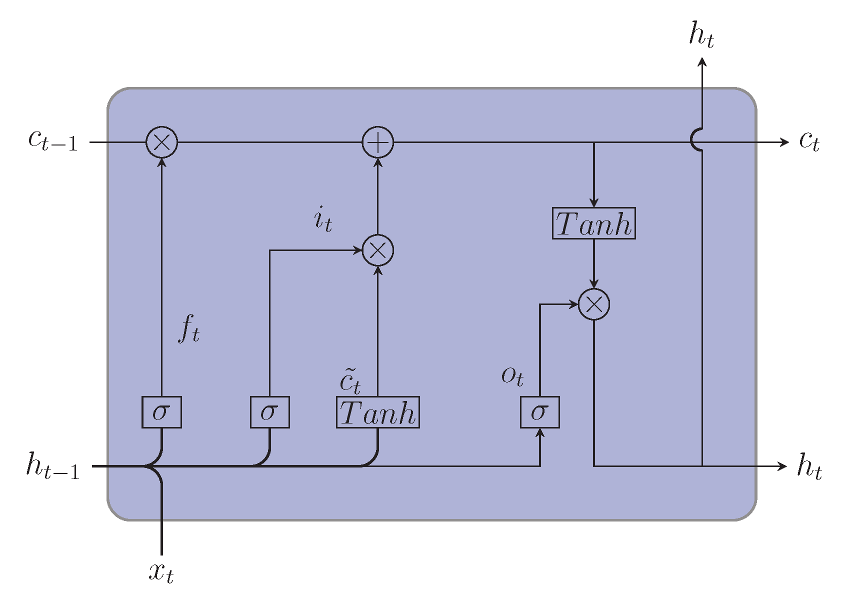
LSTM is a type of RNN that is developed to eradicate the shortcoming of RNN to learn long-term dependencies [34,35]. Due to remembering information for a long time and removing the vanishing gradient problem of RNN, LSTM has appeared to be an effective model in solving problems with sequential data containing long-term dependencies. Some of the examples of LSTM applications are speech recognition [36], machine translation [37], time series forecasting [38,39], and sentiment analysis [40]. Hochreiter and Schmidhuber [41] in 1997 first proposed the LSTM model in which each LSTM unit contains only input and output gates. This model was later refined by Gers et al. [42], who introduced a forget gate in LSTM unit. The components of LSTM unit containing cell state, hidden state, and different gates are illustrated in Figure 1. Cell state carries the relevant information from one LSTM unit to another LSTM unit, while gates are used to regulate the addition and deduction of information to the cell state. First, the forget gate removes unnecessary information from the cell state. Information from the previous hidden state and current input state is passed through sigmoid function, resulting in values between 0 and 1. Next, the input gate determines what new information will be added to the cell state. The old cell state is then updated to a new cell state by combining input and forget gate information. Finally, the output gate returns the new hidden state. The mathematical equation of the input gate , the forget gate , the output gate , the cell state , and the hidden state at time step t are as follows [43]:
where is the input at time step t, is the output at time step , denotes the sigmoid function, and denotes hyperbolic tangent activation function. The weight matrices are , , , and ; corresponding bias vectors are , , , and . Temporary memory cell state at t is , and final cell output is .
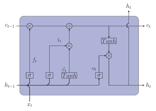
Figure 1.
Architecture of LSTM.
4. Methodology
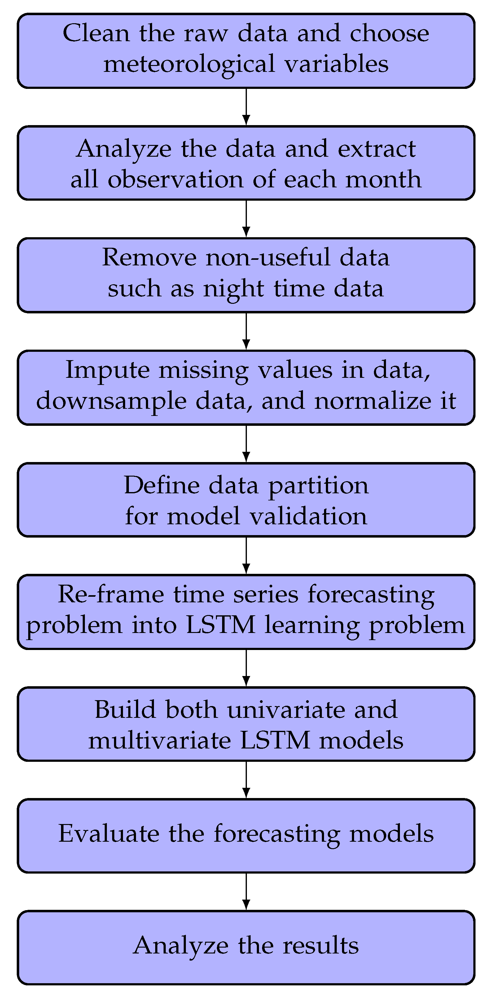
This section describes the methodology of the proposed LSTM framework for very short-term GHI prediction. The overall process flow is shown in Figure 2. At the beginning, the raw data are cleaned, and the observations per second are taken containing GHI and three additional meteorological variables (temperature, wind direction, and humidity) in a year. We then analyze the variation of meteorological variables in each month and create 12 datasets. Following this, we remove the useless data such as nighttime data from the datasets, impute missing data values using interpolation, reduce the number of samples from one-minute intervals to five-minute intervals, and normalize the data. The next step is partitioning the data using cross-validation for model validation techniques, followed by transforming the time series problem into a supervised learning problem. We then construct multivariate and univariate LSTM models. In multivariate case, we consider possible combinations of meteorological variables. Finally, after building the models, we evaluate them and analyze the obtained results. The details are presented below.
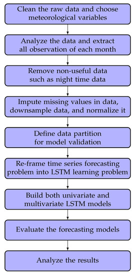
Figure 2.
Process flow of the proposed approach.
4.1. Data Collection
Our selected data contain weather observation from 1 January 2016 to 31 December 2016 at Guntur in the Indian state of Andhra Pradesh (latitude [N] 16.37 and longitude [E] 80.53). We have collected the data from the solar radiation resource assessment (SRRA) stations in India (http://niwe.res.in accessed on 1 May 2021) [44]. This time series data has several time-dependent variables observed per minute, from which we collect the observations with GHI, temperature, wind direction, and humidity variables.
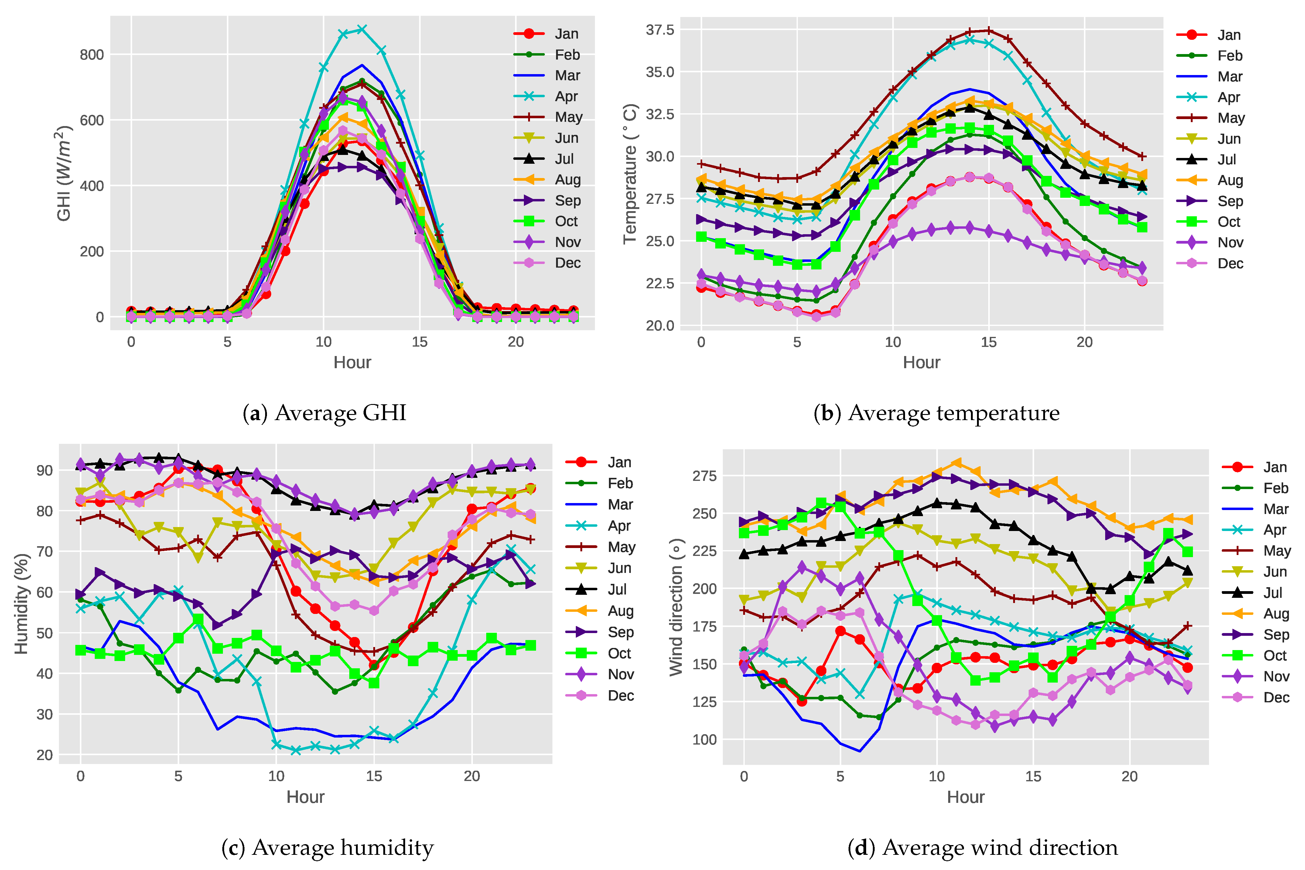
Figure 3 shows the average hourly meteorological values for each month in Guntur in 2016. It is clear from Figure 3a that for all months, the GHI value is near zero before sunrise and after sunset. The GHI values increase gradually from morning to reach their peak at noon, followed by a gradual decrease until evening. The highest GHI variation is observed in April, whereas the lowest GHI is detected in September. The amount of GHI changes in one month can be different from in another month, and these changes may be due to the variation in weather patterns.
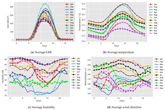
Figure 3.
Average hourly meteorological values for each month in Guntur in 2016.
Figure 3b shows that the temperature is the highest around noon every day because the sun rays fall directly on earth in the middle of the day. It is clear that the temperature is relatively high from April to May due to summer season in Guntur. On the other hand, the temperature in this region is relatively low during the winter season from November to January.
In terms of hourwise average humidity of each of the months, Figure 3c does not show any clear trend, but in general, humidity is relatively low during daytime compared to nighttime. The lowest humidity is found in April, whereas July and November have the highest humidity value.
Similarly, hourwise wind direction does not show any clear pattern (Figure 3d). Some months, such as August and September, have less fluctuation of wind direction. On the other hand, in November, December, March, and April, wind direction varied throughout the day.
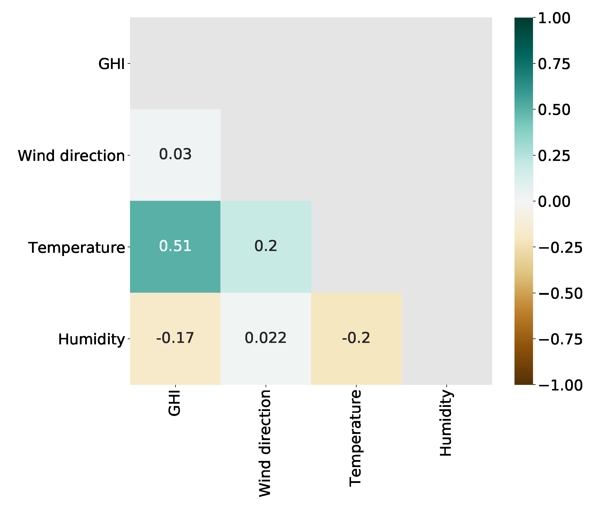
Moreover, the correlation among the variables is shown in Figure 4. It shows that there is a positive correlation exists between GHI and temperature. Moreover, GHI has a weak negative correlation with humidity and almost no correlation with wind direction. Similarly, there is little correlation can be found between wind direction and humidity. The temperature, on the other hand, is positively correlated with wind direction but negatively correlated with humidity.

Figure 4.
Correlation matrix among the variables.
4.2. Data Prepossessing
The raw data that we obtained contain observations with four variables. The first step was to clean up the data by deleting ambiguous or irrelevant records. The data also include some missing values, which were processed by the linear interpolation method. Then we create 12 datasets from the processed data so that each data set contains all the observations for a specific month. In the original dataset, observations were recorded at one-minute intervals. Therefore, the total number of observations for a month with 31 days is 44,640, for a month with 30 days is 43,200, and for a month with 29 days is 41,760. As the variations of consecutive GHI values are relatively close, we use the mean of 5 min intervals as a new single observation. We have deleted all observations with zero GHI values at the beginning and end of the day since the GHI values after sunset are zero. However, we have not omitted any observations with a zero GHI value after obtaining at least one non-zero GHI value. Table 1 shows the description of all 12 datasets, which includes the name of the months, duration of data, the total number of samples (after downsampling and removing nighttime data), and the number of input variables.

Table 1.
Description of the data.
We also normalized the data set using Min–Max normalization, which scales the data between 0 and 1 so that all variables are processed similarly for machine learning model building. The formula of Min–Max normalization is as follows:
where v indicates normalized value of a variable, and are one and zero, respectively. The current, minimum and maximum value of the variable before normalization are x, and , respectively.
4.3. Data Partitioning
To evaluate the performance of the models, we have used ten-fold cross-validation. First, we divided each dataset into ten equal subsets, each of which contains 10% of data. Next, we selected nine subsets to train the models and another subset to test the models. We then repeated the process ten times to ensure that all folds were included as a test set. Finally, we find the performance metric for the model by averaging the results obtained in these ten iterations.
4.4. Proposed Univariate vs. Multivariate LSTM Models
In this subsection, we propose predictive frameworks to forecast GHI using the univariate and multivariate LSTM models. After the completion of preprocessing and data partitioning, the time series data contained observations of GHI, temperature, humidity, and wind direction features at each time step. To perform GHI prediction, we had to re-frame the time series data into supervised learning datasets. This process was performed by a sliding window method in which future time steps are predicted using prior time steps. As we consider very short-term GHI prediction, we have used a multi-step forecast, which means predicting a few future times-steps. To predict GHI, we have built one univariate and seven multivariate LSTM models. In the univariate model, the input vector considers only the GHI variable. On the other hand, each multivariate LSTM input vector contains GHI variable along with a possible combination of temperature, humidity, and wind direction variable. Except for these differences, the structure of all the models is the same. Table 2 shows the name of each model, its type, and input and output vectors. In this table, t indicates the current time step, where n is the lag values or window size, and m indicates the future steps. Furthermore, , , , and represent global horizontal irradiance, temperature, humidity, and wind direction, respectively.
Table 2.
Input and output vector of univariate and different multivariate LSTM models.
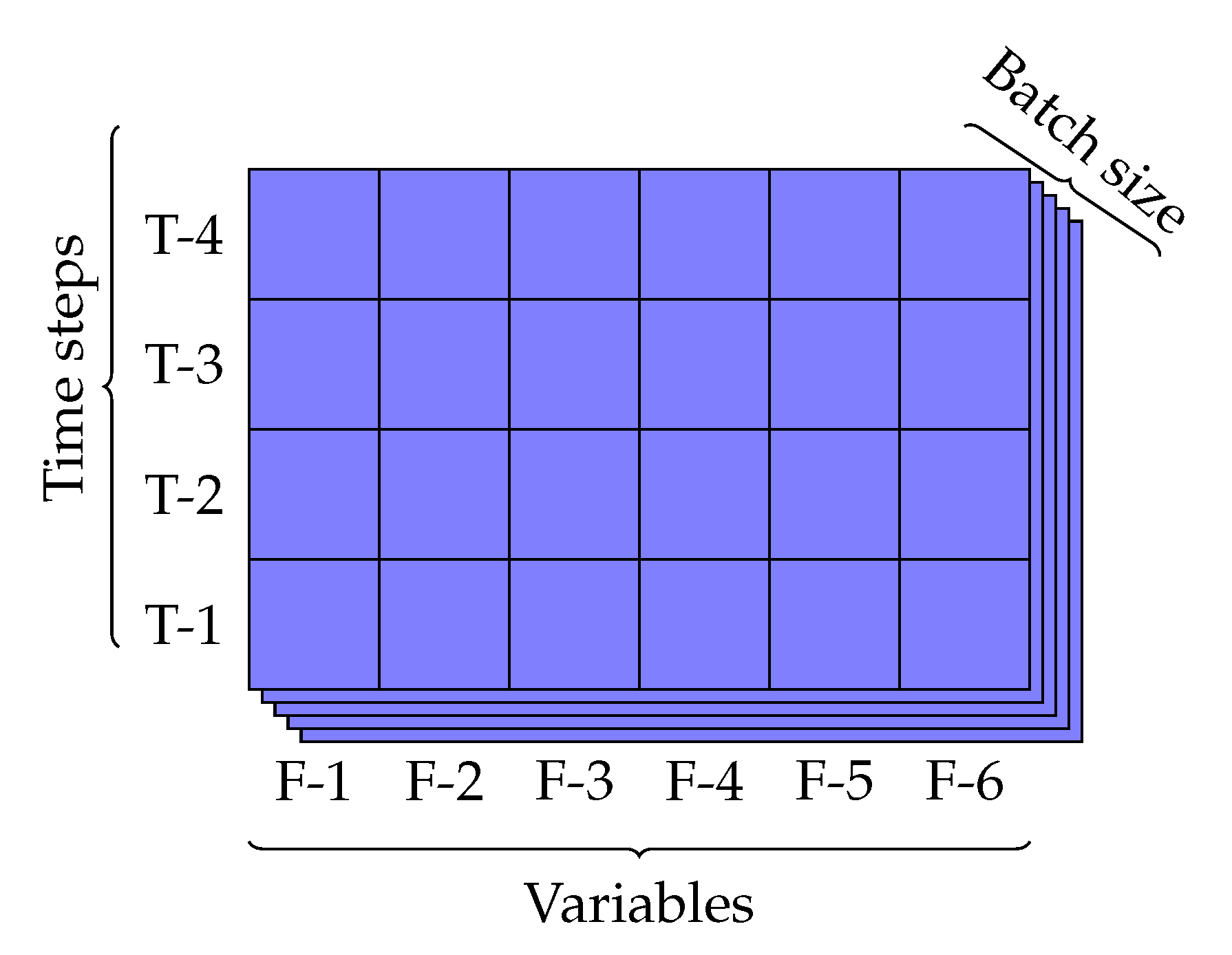
To build the LSTM models, we needed to restructure data into a three-dimensional array. These three dimensions are the number of input variables, the number of time-steps (window size), and the number of samples (batch size). For example, a 3D array that has shape (72, 2, 25) means that input data has a batch size of 72 (72 observations for each batch), two variables, and 25 time-steps. Figure 5 shows the 3D input structure with shape (5, 6, 4).
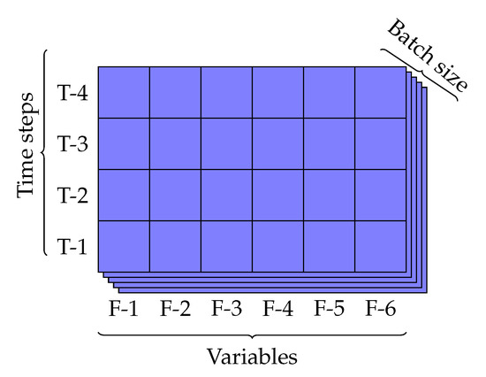
Figure 5.
3D input in a LSTM model.
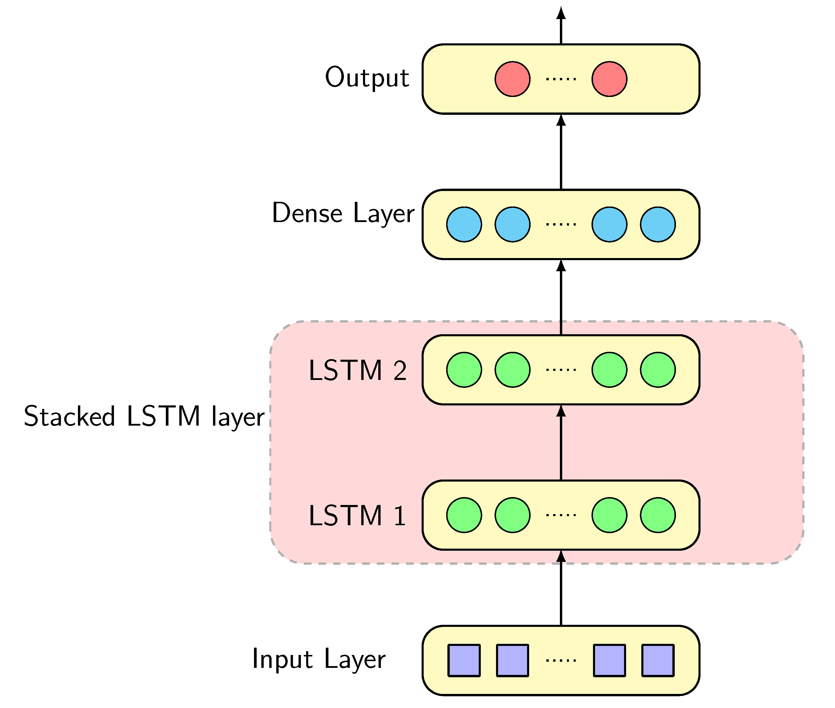
Figure 6 shows the architecture of each of the models in which we employ a stacked LSTM. First, 3D input vectors are fed into the input layer. Following this, the input layer passes the data into a stacked LSTM layer that consists of two hidden layers, each containing 50 LSTM neurons. After taking the output of the first LSTM layer as its input, the second LSTM layer is then connected to the dense layer, a fully connected neural network. Finally, the output of the dense layer produces the forecast values. Our output node varies from 1 to 24 based on desired future time-steps, which means that we can predict GHI up to 2 h ahead. It is noted that one step ahead prediction means five minute ahead prediction. In these models, is used as an activation function for each hidden layer, Adam is used as a gradient optimization algorithm, and mean square error (MSE) is used as a loss function.
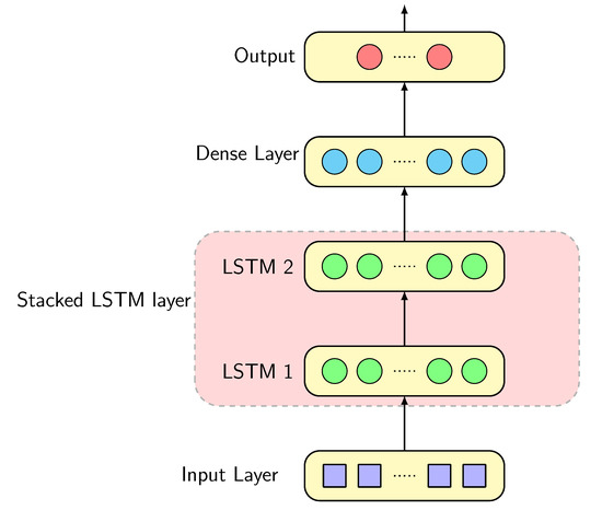
Figure 6.
Proposed LSTM architecture.
In the LSTM models, we used the training dataset to build each model and testing dataset to predict, with the number of epochs being set to 100. We also initialized the batch size as 32 and fixed the window size at 35 to perform the short-term GHI prediction. Table 3 shows the hyper-parameters we set for both univariate and multivariate LSTM models. Hyper-parameters such as batch size, number of epoch, window size, and number of hidden layer were defined based on some preliminary experiments. To tune these hyper-parameters, we tried ten probable candidate values and finally choose the value that produces the best result. For other hyper-parameters, we adopted the values from [45].
Table 3.
Hyper-parameters used for univariate and multivariate LSTM models.
We used the Root Mean Squared Error (RMSE) and MAE to evaluate the prediction performances of the models.
where and y represent the ith forecasted and measured values, respectively, and N is the total number of observations.
To identify any correlation between variables of the dataset, we used Pearson correlation coefficient. If the number of samples is n, then the correlation coefficient r between two variables x and y is measured with the following equation:
where and represent mean values of feature x and y, respectively.
We did the simulation with AMD Ryzen 9 processor, 128 GB RAM, Unbuntu 20.4 64-bit OS, using Python 3.7.1. In addition, we employed SKlearn library for several data preprocessing tasks and Keras library for implementing LSTM network. To obtain reliable results, we ran the simulation twenty times with twenty random seeds and recorded the average, minimum, and maximum RMSE along with MAE for each LSTM model in forecasting GHI.
5. Result Analysis and Discussion
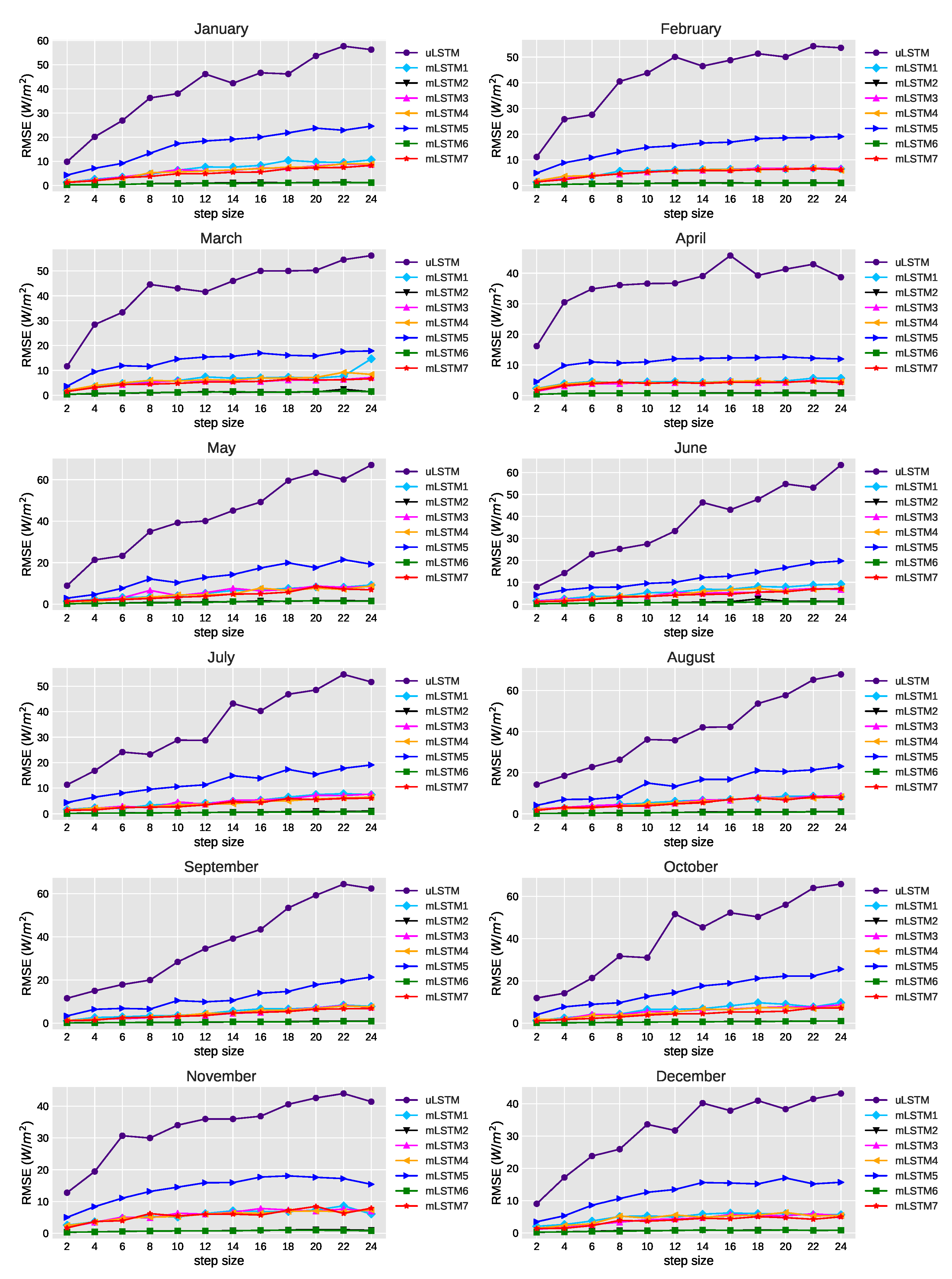
Figure 7 shows the changes of average RMSE values of the univariate and multivariate models where the future step size is increased from 2 to 24. Considering the multi-step ahead forecasting for all models, we found that errors increased as the number of steps increased. The univariate model performed worse than others with the increase of step size for all of the months. Moreover, among the multivariate approaches, mLSTM2 and mLSTM6 exhibited lower average RMSE values compared to other multivariate models. In these two models, average RMSE did not increase significantly with the increase of step size. In addition, mLSTM5 did not perform as good as other multivariate models for all the months.
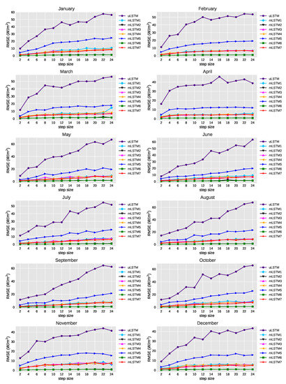
Figure 7.
Average RMSE (W/m) for different steps-ahead prediction of GHI using the selected models.
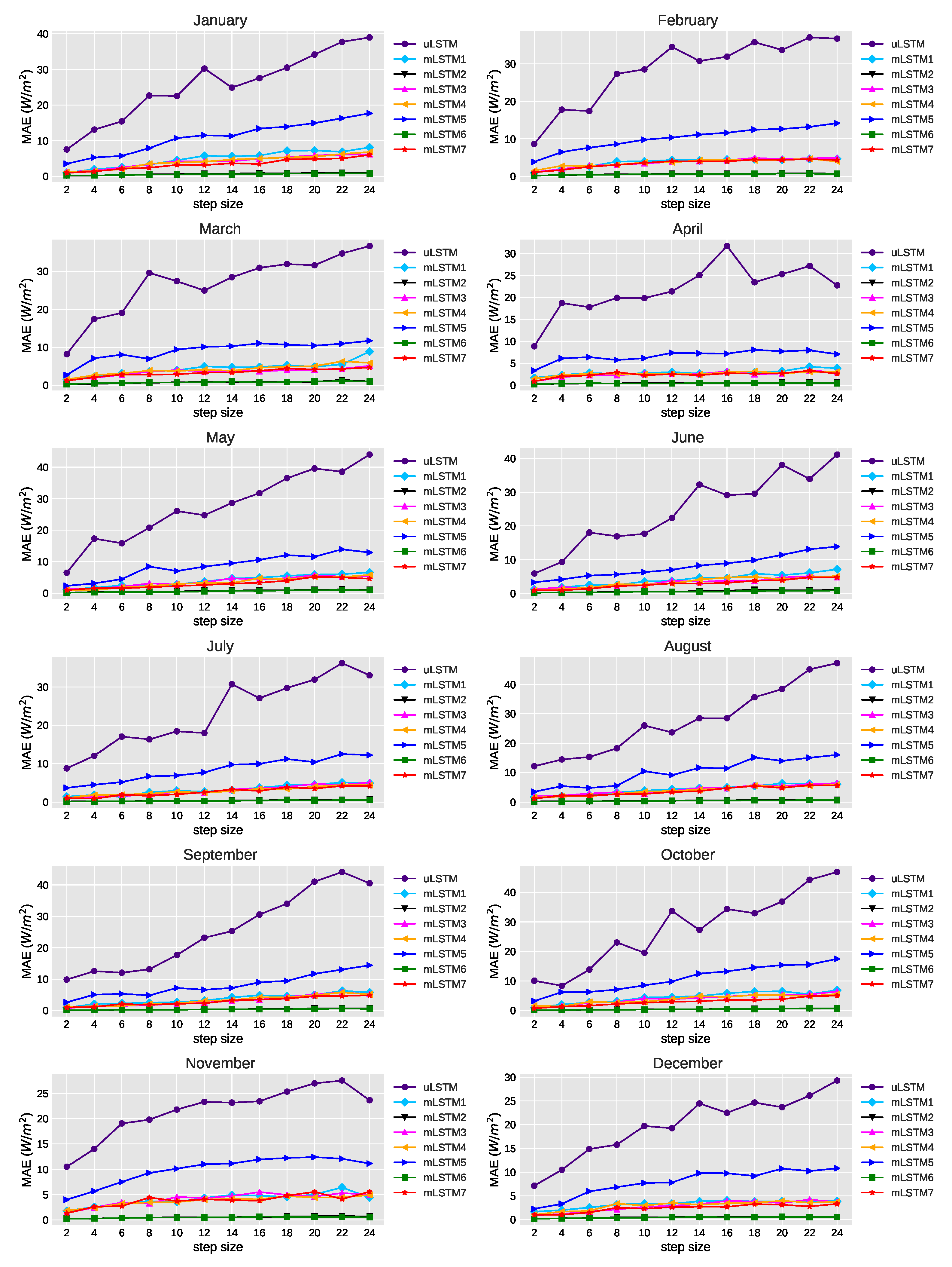
Figure 8 illustrates the effect of average MAE values when step size was increased from 2 to 24. It is clearly shown that average MAE of the univariate model for any step size is far higher than average MAE of any of the multivariate models. Moreover, mLSTM5 has a higher average MAE than other multivariate models. We also see that regarding average MAE, mLSTM2 and mLSTM6 have reported relatively small errors.
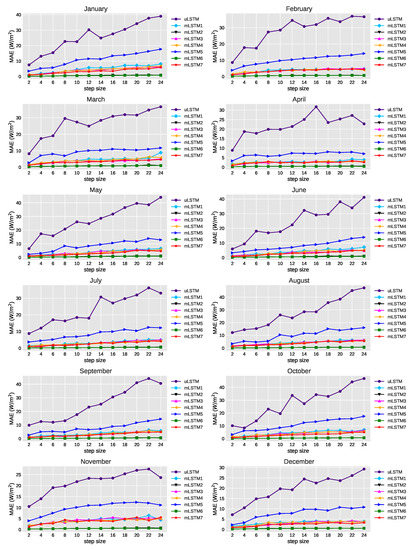
Figure 8.
Average MAE (W/m) for different steps-ahead prediction of GHI using the selected models.
Table 4 shows the average, minimum, and maximum RMSE for the proposed models in predicting short-term GHI (24 future steps). It is obvious that for the long term GHI, the uLSTM model outperforms mLSTM models. This is because in all months, average RMSE values for uLSTM are 67.91 W/m to 38.69 W/m, which are much higher than the average RMSE values of any other multivariate model. The best performing model is mLSTM6, producing average RMSE ranging 0.74 W/m–1.150 W/m followed by mLSTM2, which shows competitive average RMSE values with mLSTM6 (0.87 W/m–1.53 W/m). The average RMSE values of mLSTM5, which is from 11.96 W/m to 25.56 W/m, is the highest among the multivariate models, whereas the other four models mLSTM1, mLSTM3, mLSTM4, and mLSTM7 show moderate performances.
Table 4.
Average, minimum, and maximum RMSE (W/m) for LSTM models during very short-term GHI prediction (24 future steps or 2 h ahead).
Table 5 summarizes the average, minimum and maximum MAE of the approaches regarding very short-term prediction. The average MAE values also indicate that uLSTM becomes the worst among the models, obtaining average MAE scores of 22.78 W/m–47.31 W/m, much higher compared to its multivariate counterparts. Among the multivariate LSTM models, mLSTM5 is not as effective as other models, producing higher average MAE values (7.09 W/m–17.71 W/m) compared to other multivariate methods. In terms of MAE, the two best performing models are mLSTM6 and MLSTM2, having the MAE scores of 0.45 W/m–1.01 W/m and 0.56 W/m–1.11 W/m, respectively. Reset of the multivariate models shows slightly worse performance.
Table 5.
Average, minimum, and maximum MAE (W/m) for LSTM models during very short-term prediction (24 future steps or 2 h ahead).
The boxplot in Figure 9 shows the overall RMSE obtained by uLSTM and seven mLSTM (mLSTM1-mLSTM7) models for the very short-term prediction task, with only average RMSE considered. We can observe from the median value that model mLSTM6 and mLSTM2 yield the best forecasting results compared to other multivariate models. In addition, the variation of RMSE for these two is much lower than that of other approaches. The univariate model uLSTM has the largest median values of RMSE, and the variation in RMSE is also the highest. The relatively lower inter-quartile range regarding RMSE for mLSTM2 and mLSTM6 suggest that both are stable in predicting GHI in all weather condition (i.g., over the year).
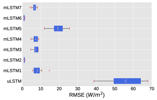
Figure 9.
RMSE (W/m) boxplot for both univariate and multivariate models for very short-term prediction.
Based on the experimental results, it is evident that multivariate models are better than the univariate model. However, not all multivariate LSTM models perform equally better when we compared among them. The best-performing model mLSTM6 contains temperature with GHI as an input variable. Its best performance ability might be attributed to the relatively better positive correlation between these two variables. The second-best-performing model mLSTM2 has GHI and temperature along with wind direction as input. Here, temperate is positively correlated with both GHI and wind direction. Among the multivariate models, mLSTM5 is the worst-performing model, and it has GHI and wind direction as input variables. One possible explanation for the performance degradation of this model is that there is little correlation between the two variables.
6. Conclusions and Future Work
This paper has presented a comparative analysis between univariate and multivariate LSTM models for predicting very short-term GHI. To validate our proposed approaches, we collected time-variant data of GHI and other weather variables from Guntur in India from 1 January 2016 to 31 December 2016. We split the data and built 12 datasets, with each dataset containing minutewise observations of a month. The univariate LSTM considered only GHI variable for input data. On the other hand, multivariate LSTM models used GHI variable and all possible combinations of other meteorological variables (temperature, wind direction and humidity), thus producing seven multivariate models. Before building the models, we pre-processed the datasets and transformed them to supervise learning problem datasets. As a result, each LSTM model can adequately use the datasets to build a prediction model. Furthermore, to achieve very short-term GHI prediction, we considered multi-step forecasting to predict up to 24 steps in the future.
Our experimental result shows that each multivariate model outperforms the univariate model in predicting very short-term GHI. Among the multivariate models, mLSTM6 shows the lowest forecasting error, followed by mLSM2. These two multivariate models perform much better than the other five models because the integration of temperature data with GHI as input and both wind direction and temperature data with GHI as input tends to be effective for multi-step ahead GHI prediction. Although multivariate models exhibit better performance than the univariate model, they take more time for training due to added input variables.
In the experiments, we set the hyper-parameters of the models based on some preliminary experiments. However, considering grid search or other optimization algorithms to find the appropriate parameters might improve the performance of the models. Furthermore, we employed data from one station for evaluating the model due to the availability of the data, but we will use data from other stations for different months in future study. We will also investigate the viability of other deep learning models such as CNN and GRU for the very short-term GHI prediction.
Author Contributions
Conceptualization, A.K.M., R.S., S.G. and B.C.; methodology, A.K.M. and R.S.; software, A.K.M.; validation, A.K.M., R.S. and B.C.; writing—original draft preparation, A.K.M.; writing—review and editing, B.C.; supervision, B.C.; funding acquisition, B.C. All authors have read and agreed to the published version of the manuscript.
Funding
This research was supported by Iwate Prefectural University general research fund.
Institutional Review Board Statement
Not applicable.
Informed Consent Statement
Not applicable.
Data Availability Statement
The data that support the findings of this study are available on request from the corresponding author.
Acknowledgments
The authors acknowledge the resources and support provided by Pattern Recognition and Machine Learning laboratory, Department of Software and Information Science, Iwate Prefectural University. The authors also thank anonymous referees for their valuable comments.
Conflicts of Interest
The authors declare no conflict of interest.
Abbreviations
The following abbreviations are used in this manuscript:
| ANN | Artificial neural network |
| ARIMA | Autoregressive integrated moving average |
| CNN | Convolutional neural network |
| DHI | Diffuse horizontal irradiance |
| DNI | Direct normal irradiance |
| DNN | Deep neural network |
| ETS | Exponential smoothing |
| GA | Genetic algorithm |
| GARCH | Generalized autoregressive conditional heteroskedasticity |
| GBR | Gradient boosting regression |
| GHI | Global horizontal irradiance |
| GPR | Gaussian process regression |
| GRU | Gated recurrent units |
| KNN | K-nearest neighbour |
| LSTM | Long short-term memory |
| MAE | Mean absolute error |
| MSE | Mean squared error |
| MLP | Multilayer perceptron |
| NSGA II | Non-dominated sorting genetic algorithm II |
| PV | Photovoltaic |
| PSO | Particle swarm optimization |
| ReLU | Rectified linear unit |
| RF | Random forest |
| RMSE | Root mean square error |
| RNN | Recurrent neural network |
| SRRA | Solar radiation resource assessment |
| SVM | Support vector machine |
| SVR | Support vector regression |
| XGBoost | Extreme gradient boosting |
References
- Bot, K.; Ruano, A.; Ruano, M.D.G. Short-Term Forecasting Photovoltaic Solar Power for Home Energy Management Systems. Inventions 2021, 6, 12. [Google Scholar] [CrossRef]
- Kallio-Myers, V.; Riihelä, A.; Lahtinen, P.; Lindfors, A. Global horizontal irradiance forecast for Finland based on geostationary weather satellite data. Sol. Energy 2020, 198, 68–80. [Google Scholar] [CrossRef]
- Panda, M.; Das, B.; Pati, B.B. A Hybrid Approach for Path Planning of Multiple AUVs. In Innovation in Electrical Power Engineering, Communication, and Computing Technology; Springer: Berlin, Germany, 2020; pp. 327–338. [Google Scholar]
- Nespoli, L.; Medici, V. An unsupervised method for estimating the global horizontal irradiance from photovoltaic power measurements. Sol. Energy 2017, 158, 701–710. [Google Scholar] [CrossRef] [Green Version]
- Alsharif, M.H.; Younes, M.K.; Kim, J. Time Series ARIMA Model for Prediction of Daily and Monthly Average Global Solar Radiation: The Case Study of Seoul, South Korea. Symmetry 2019, 12, 240. [Google Scholar] [CrossRef] [Green Version]
- Kumar Barik, A.; Malakar, S.; Goswami, S.; Ganguli, B.; Sen Roy, S.; Chakrabarti, A. Analysis of GHI Forecasting Using Seasonal ARIMA. In Data Management, Analytics and Innovation; Sharma, N., Chakrabarti, A., Balas, V.E., Martinovic, J., Eds.; Springer: Singapore, 2021; pp. 55–69. [Google Scholar]
- Dong, Z.; Yang, D.; Reindl, T.; Walsh, W.M. Short-term solar irradiance forecasting using exponential smoothing state space model. Energy 2013, 55, 1104–1113. [Google Scholar] [CrossRef]
- Sun, H.; Yan, D.; Zhao, N.; Zhou, J. Empirical investigation on modeling solar radiation series with ARMA–GARCH models. Energy Convers. Manag. 2015, 92, 385–395. [Google Scholar] [CrossRef]
- Mellit, A.; Pavan, A.M. A 24-h forecast of solar irradiance using artificial neural network: Application for performance prediction of a grid-connected PV plant at Trieste, Italy. Sol. Energy 2010, 84, 807–821. [Google Scholar] [CrossRef]
- Zendehboudi, A.; Baseer, M.; Saidur, R. Application of support vector machine models for forecasting solar and wind energy resources: A review. J. Clean. Prod. 2018, 199, 272–285. [Google Scholar] [CrossRef]
- Chen, C.R.; Kartini, U.T. K-Nearest neighbor neural network models for very short-term global solar irradiance forecasting based on meteorological data. Energies 2017, 10, 186. [Google Scholar] [CrossRef] [Green Version]
- Benali, L.; Notton, G.; Fouilloy, A.; Voyant, C.; Dizene, R. Solar radiation forecasting using artificial neural network and random forest methods: Application to normal beam, horizontal diffuse and global components. Renew. Energy 2019, 132, 871–884. [Google Scholar] [CrossRef]
- Alzahrani, A.; Shamsi, P.; Dagli, C.; Ferdowsi, M. Solar irradiance forecasting using deep neural networks. Procedia Comput. Sci. 2017, 114, 304–313. [Google Scholar] [CrossRef]
- Dong, N.; Chang, J.F.; Wu, A.G.; Gao, Z.K. A novel convolutional neural network framework based solar irradiance prediction method. Int. J. Electr. Power Energy Syst. 2020, 114, 105411. [Google Scholar] [CrossRef]
- Li, G.; Wang, H.; Zhang, S.; Xin, J.; Liu, H. Recurrent Neural Networks Based Photovoltaic Power Forecasting Approach. Energies 2019, 12, 2538. [Google Scholar] [CrossRef] [Green Version]
- Yu, X.; Ho, H.; Hung, V.; Lee, G.; Jung, S. Application of Long Short-Term Memory (LSTM) Neural Network for Flood Forecasting. Water 2019, 11, 1387. [Google Scholar] [CrossRef] [Green Version]
- Brahma, B.; Wadhvani, R. Solar Irradiance Forecasting Based on Deep Learning Methodologies and Multi-Site Data. Symmetry 2020, 12, 1830. [Google Scholar] [CrossRef]
- Jeon, B.k.; Kim, E.J. Next-Day Prediction of Hourly Solar Irradiance Using Local Weather Forecasts and LSTM Trained with Non-Local Data. Energies 2020, 13, 5258. [Google Scholar] [CrossRef]
- Wang, F.; Mi, Z.; Su, S.; Zhao, H. Short-Term Solar Irradiance Forecasting Model Based on Artificial Neural Network Using Statistical Feature Parameters. Energies 2012, 5, 1355–1370. [Google Scholar] [CrossRef] [Green Version]
- Notton, G.; Voyant, C.; Fouilloy, A.; Duchaud, J.L.; Nivet, M.L. Some Applications of ANN to Solar Radiation Estimation and Forecasting for Energy Applications. Appl. Sci. 2019, 9, 209. [Google Scholar] [CrossRef] [Green Version]
- Nalina, U.; Prema, V.; Smitha, K.; Rao, K.U. Multivariate regression for prediction of solar irradiance. In Proceedings of the 2014 International Conference on Data Science Engineering (ICDSE), Kochi, India, 26–28 August 2014; pp. 177–181. [Google Scholar] [CrossRef]
- Mujabar, S.; Chintaginjala Venkateswara, R. Empirical models for estimating the global solar radiation of Jubail Industrial City, the Kingdom of Saudi Arabia. SN Appl. Sci. 2021, 3, 95. [Google Scholar] [CrossRef]
- Jadidi, A.; Menezes, R.; De Souza, N.; De Castro Lima, A.C. A Hybrid GA–MLPNN Model for One-Hour-Ahead Forecasting of the Global Horizontal Irradiance in Elizabeth City, North Carolina. Energies 2018, 11, 2641. [Google Scholar] [CrossRef] [Green Version]
- Dash, S.; Satpathy, P.R.; Panda, S.; Sharma, R. Global Horizontal Irradiance Prediction Using Deep Neural Network Framework. In Innovation in Electrical Power Engineering, Communication, and Computing Technology; Springer: Berlin, Germany, 2020; pp. 317–326. [Google Scholar]
- Kumari, P.; Toshniwal, D. Extreme gradient boosting and deep neural network based ensemble learning approach to forecast hourly solar irradiance. J. Clean. Prod. 2021, 279, 123285. [Google Scholar] [CrossRef]
- Yadav, A.P.; Kumar, A.; Behera, L. RNN based solar radiation forecasting using adaptive learning rate. In International Conference on Swarm, Evolutionary, and Memetic Computing; Springer: Berlin, Germany, 2013; pp. 442–452. [Google Scholar]
- Husein, M.; Chung, I.Y. Day-Ahead Solar Irradiance Forecasting for Microgrids Using a Long Short-Term Memory Recurrent Neural Network: A Deep Learning Approach. Energies 2019, 12, 1856. [Google Scholar] [CrossRef] [Green Version]
- Abdel-Nasser, M.; Mahmoud, K.; Lehtonen, M. Reliable Solar Irradiance Forecasting Approach Based on Choquet Integral and Deep LSTMs. IEEE Trans. Ind. Inform. 2021, 17, 1873–1881. [Google Scholar] [CrossRef]
- Srivastava, S.; Lessmann, S. A comparative study of LSTM neural networks in forecasting day-ahead global horizontal irradiance with satellite data. Sol. Energy 2018, 162, 232–247. [Google Scholar] [CrossRef]
- Yu, Y.; Cao, J.; Zhu, J. An LSTM Short-Term Solar Irradiance Forecasting Under Complicated Weather Conditions. IEEE Access 2019, 7, 145651–145666. [Google Scholar] [CrossRef]
- Boubaker, S.; Benghanem, M.; Mellit, A.; Lefza, A.; Kahouli, O.; Kolsi, L. Deep Neural Networks for Predicting Solar Radiation at Hail Region, Saudi Arabia. IEEE Access 2021, 9, 36719–36729. [Google Scholar] [CrossRef]
- Hosseini, M.; Katragadda, S.; Wojtkiewicz, J.; Gottumukkala, R.; Maida, A.; Chambers, T.L. Direct Normal Irradiance Forecasting Using Multivariate Gated Recurrent Units. Energies 2020, 13, 3914. [Google Scholar] [CrossRef]
- Zang, H.; Liu, L.; Sun, L.; Cheng, L.; Wei, Z.; Sun, G. Short-term global horizontal irradiance forecasting based on a hybrid CNN-LSTM model with spatiotemporal correlations. Renew. Energy 2020, 160, 26–41. [Google Scholar] [CrossRef]
- Yu, Y.; Si, X.; Hu, C.; Zhang, J. A review of recurrent neural networks: LSTM cells and network architectures. Neural Comput. 2019, 31, 1235–1270. [Google Scholar] [CrossRef]
- Kratzert, F.; Klotz, D.; Brenner, C.; Schulz, K.; Herrnegger, M. Rainfall–Runoff modelling using Long Short-Term Memory (LSTM) networks. Hydrol. Earth Syst. Sci. 2018, 22, 6005–6022. [Google Scholar] [CrossRef] [Green Version]
- Jo, J.; Kung, J.; Lee, Y. Approximate LSTM Computing for Energy-Efficient Speech Recognition. Electronics 2020, 9, 2004. [Google Scholar] [CrossRef]
- Su, C.; Huang, H.; Shi, S.; Jian, P.; Shi, X. Neural machine translation with Gumbel Tree-LSTM based encoder. J. Vis. Commun. Image Represent. 2020, 71, 102811. [Google Scholar] [CrossRef]
- Chimmula, V.K.R.; Zhang, L. Time series forecasting of COVID-19 transmission in Canada using LSTM networks. Chaos Solitons Fractals 2020, 135, 109864. [Google Scholar] [CrossRef]
- Sezer, O.B.; Gudelek, M.U.; Ozbayoglu, A.M. Financial time series forecasting with deep learning: A systematic literature review: 2005–2019. Appl. Soft Comput. 2020, 90, 106181. [Google Scholar] [CrossRef] [Green Version]
- Huang, F.; Li, X.; Yuan, C.; Zhang, S.; Zhang, J.; Qiao, S. Attention-Emotion-Enhanced convolutional LSTM for sentiment analysis. IEEE Trans. Neural Netw. Learn. Syst. 2021. [Google Scholar] [CrossRef] [PubMed]
- Hochreiter, S.; Schmidhuber, J. Long short-Term memory. Neural Comput. 1997, 9, 1735–1780. [Google Scholar] [CrossRef]
- Gers, F.A.; Schmidhuber, J.; Cummins, F. Learning to forget: Continual prediction with LSTM. Neural Comput. 2000, 12, 2451–2471. [Google Scholar] [CrossRef]
- Li, T.; Hua, M.; Wu, X. A Hybrid CNN-LSTM Model for Forecasting Particulate Matter (PM2.5). IEEE Access 2020, 8, 26933–26940. [Google Scholar] [CrossRef]
- Kumar, A.; Gomathinayagam, S.; Giridhar, G.; Mitra, I.; Vashistha, R.; Meyer, R.; Schwandt, M.; Chhatbar, K. Field Experiences with the Operation of Solar Radiation Resource Assessment Stations in India. Energy Procedia 2014, 49, 2351–2361. [Google Scholar] [CrossRef] [Green Version]
- Malakar, S.; Goswami, S.; Ganguli, B.; Chakrabarti, A.; Roy, S.S.; Boopathi, K.; Rangaraj, A.G. Designing a long short-term network for short-term forecasting of global horizontal irradiance. SN Appl. Sci. 2021, 3, 477. [Google Scholar] [CrossRef]

Publisher’s Note: MDPI stays neutral with regard to jurisdictional claims in published maps and institutional affiliations. |
© 2021 by the authors. Licensee MDPI, Basel, Switzerland. This article is an open access article distributed under the terms and conditions of the Creative Commons Attribution (CC BY) license (https://creativecommons.org/licenses/by/4.0/).