Some Identities Involving Degenerate q-Hermite Polynomials Arising from Differential Equations and Distribution of Their Zeros

Abstract

This paper intends to define degenerate q-Hermite polynomials, namely degenerate q-Hermite polynomials by means of generating function. Some significant properties of degenerate q-Hermite polynomials such as recurrence relations, explicit identities and differential equations are established. Many mathematicians have been studying the differential equations arising from the generating functions of special numbers and polynomials. Based on the results so far, we find the differential equations for the degenerate q-Hermite polynomials. We also provide some identities for the degenerate q-Hermite polynomials using the coefficients of this differential equation. Finally, we use a computer to view the location of the zeros in degenerate q-Hermite equations. Numerical experiments have confirmed that the roots of the degenerate q-Hermit equations are not symmetric with respect to the imaginary axis.

1. Introduction

Hermite polynomials are classic orthogonal polynomials, and many studies have been conducted by various mathematicians. These Hermite polynomials also have many applications such as in physics and probability theory (see [1,2,3,4,5,6,7,8,9,10,11]). Throughout this paper, $\mathbb{C}$ indicates the set of complex numbers and $\mathbb{R}$ designates a set of real numbers. Furthermore, the variable $q\in \mathbb{C}$, such that $\left|q\right|<1$. q-analogues of $x\in \mathbb{C}$ is specified as

$${\left[x\right]}_q=\frac{1-q^x}{1-q}.$$

Note that ${lim}_{q\to 1}{\left[x\right]}_q=x.$

The q-Hermite polynomials ${\mathbf{H}}_{n,q}\left(x\right)$ [11,12] are defined by

$${\mathbf{H}}_{n,q}\left(x\right)=n!{\displaystyle \sum _{k=0}^{\left[\frac{n}{2}\right]}}{\displaystyle \frac{{(-1)}^k{2}^{n-2k}{\left[x\right]}_q^{n-2k}}{k!(n-2k)!}}.$$

The differential equation and the generating function for ${\mathbf{H}}_{n,q}\left(x\right)$ are given by

$$\begin{array}{l}\left({\displaystyle \frac{q-1}{q^{x}logq}}{\displaystyle \frac{d^2}{d{x}^2}}+\left({\displaystyle \frac{1-q}{q^x}}-{\displaystyle \frac{2(1-q^x)}{1-q}}\right){\displaystyle \frac{d}{dx}}+2n{\displaystyle \frac{logq}{q-1}}{q}^x\right){\mathbf{H}}_{n,q}\left(x\right)=0,\\ {\mathbf{H}}_{n,q}\left(0\right)=\left\{\begin{array}{cc}{(-1)}^k{\displaystyle \frac{\left(2k\right)!}{k!}},\hfill & \mathrm{if}n=2k,\hfill \\ 0,\hfill & \mathrm{otherwise},\hfill \end{array}\right.\end{array}$$

and

$${\displaystyle \sum _{n=0}^{\infty }}{\mathbf{H}}_{n,q}\left(x\right){\displaystyle \frac{t^n}{n!}}=e^{2{\left[x\right]}_{q}t-t^2},$$

(1)

respectively.

Additionally, the polynomials ${\mathbf{H}}_{n,q}\left(x\right)$ satisfy the following differential equation

$$\begin{array}{l}\left({\left({\displaystyle \frac{d}{d{\left[x\right]}_q}}\right)}^2-2{\left[x\right]}_q\left({\displaystyle \frac{d}{d{\left[x\right]}_q}}\right)+2n\right){\mathbf{H}}_{n,q}\left(x\right)=0,\\ {\mathbf{H}}_{n,q}\left(0\right)=\left\{\begin{array}{cc}{(-1)}^k{\displaystyle \frac{\left(2k\right)!}{k!}},\hfill & \mathrm{if}n=2k,\hfill \\ 0,\hfill & \mathrm{otherwise}.\hfill \end{array}\right.\end{array}$$

Mathematicians have studied the differential equations arising from the generating functions of special numbers and polynomials (see [12,13,14]). Based on the results so far, in this work, we can derive the differential equations generated from the generating function of degenerate q-Hermite polynomials ${\mathcal{H}}_{n,q}\left(x\right|\lambda )$. By using the coefficients of this differential equation, we obtain explicit identities for the degenerate q-Hermite polynomials ${\mathcal{H}}_{n,q}\left(x\right|\lambda ).$ The rest of the paper is organized as follows. In Section 2, we derive the differential equations generated from the generating function of degenerate q-Hermite polynomials ${\mathcal{H}}_{n,q}\left(x\right|\lambda ).$ Using the coefficients of this differential equation, we obtain explicit identities for the degenerate q-Hermite polynomials ${\mathcal{H}}_{n,q}\left(x\right|\lambda ).$ In Section 3, we use the software to check the zeros of the degenerate q-Hermite equations. In addition, we observe the pattern of scattering phenomenon about the zeros of degenerate q-Hermite equations.

2. Basic Properties for the Degenerate $\mathit{q}$-Hermite Polynomials

In this section, we construct the degenerate q-Hermite polynomials ${\mathcal{H}}_{n,q}\left(x\right|\lambda )$. We obtain some properties of the degenerate q-Hermite polynomials ${\mathcal{H}}_{n,q}\left(x\right|\lambda )$.

Definition 1.

The degenerate q-Hermite polynomials ${\mathcal{H}}_{n,q}\left(x\right|\lambda )$ and degenerate q-Hermite numbers ${\mathcal{H}}_{n,q}\left(\lambda \right)$ are usually defined by the generating functions

$${(1+\lambda )}^{{\displaystyle \frac{2{\left[x\right]}_{q}t-t^2}{\lambda }}}={\displaystyle \sum _{n=0}^{\infty }}{\mathcal{H}}_{n,q}\left(x\right|\lambda ){\displaystyle \frac{t^n}{n!}},$$

(2)

and

$${(1+\lambda )}^{{\displaystyle \frac{-t^2}{\lambda }}}={\displaystyle \sum _{n=0}^{\infty }}{\mathcal{H}}_n\left(\lambda \right){\displaystyle \frac{t^n}{n!}},$$

respectively.

Clearly, ${\mathcal{H}}_n\left(\lambda \right)={\mathcal{H}}_{n,q}\left(0\right|\lambda )$.

Since ${(1+\lambda )}^{\frac{t}{\lambda }}\to e^t$ as $\lambda \to 0$, it is evident that (2) reduces to (1). We recall that the classical Stirling numbers of the first kind $S_1(n,k)$ and the second kind $S_2(n,k)$ are defined by the relations

$${\left(x\right)}_n={\displaystyle \sum _{k=0}^n}{S}_1(n,k)x^k$$

and

$$x^n={\displaystyle \sum _{k=0}^n}{S}_2(n,k){\left(x\right)}_k,$$

respectively (see [15]). Here ${\left(x\right)}_n=x(x-1)\dots (x-n+1)$ denotes the falling factorial polynomial of order n. We also have

$${\displaystyle \sum _{n=m}^{\infty }}{S}_2(n,m){\displaystyle \frac{t^n}{n!}}={\displaystyle \frac{{(e^t-1)}^m}{m!}}\mathrm{and}{\displaystyle \sum _{n=m}^{\infty }}{S}_1(n,m){\displaystyle \frac{t^n}{n!}}={\displaystyle \frac{{(log(1+t))}^m}{m!}}.$$

We also need the binomial theorem: for a variable x,

$$\begin{array}{l}{(1+\lambda )}^{{\left[x\right]}_{q}t/\lambda }={\displaystyle \sum _{m=0}^{\infty }}{\left({\displaystyle \frac{t{\left[x\right]}_q}{\lambda }}\right)}_m{\displaystyle \frac{{\lambda }^m}{m!}}\\ ={\displaystyle \sum _{m=0}^{\infty }}\left({\displaystyle \sum _{l=0}^m}{S}_1(m,l){\left({\displaystyle \frac{t{\left[x\right]}_q}{\lambda }}\right)}^l{\displaystyle \frac{{\lambda }^m}{m!}}\right)\\ ={\displaystyle \sum _{l=0}^{\infty }}\left({\displaystyle \sum _{m=l}^{\infty }}{S}_1(m,l){\left[x\right]}_q^l{\lambda }^{m-l}{\displaystyle \frac{l!}{m!}}\right){\displaystyle \frac{t^l}{l!}}.\end{array}$$

(3)

By (2) and (3), we have

$$\begin{array}{l}{\displaystyle \sum _{n=0}^{\infty }}{\mathcal{H}}_{n,q}\left(x\right|\lambda ){\displaystyle \frac{t^n}{n!}}\\ ={(1+\lambda )}^{{\displaystyle \frac{2{\left[x\right]}_{q}t}{\lambda }}}{(1+\lambda )}^{-{\displaystyle \frac{t^2}{\lambda }}}\\ ={\displaystyle \sum _{k=0}^{\infty }}{\left({\displaystyle \frac{-log(1+\lambda )}{\lambda }}\right)}^k{\displaystyle \frac{t^{2k}}{k!}}{\displaystyle \sum _{l=0}^{\infty }}\left({\displaystyle \sum _{m=l}^{\infty }}{S}_1(m,l)2^l{\left[x\right]}_q^l{\lambda }^{m-l}{\displaystyle \frac{l!}{m!}}\right){\displaystyle \frac{t^l}{l!}}\\ ={\displaystyle \sum _{n=0}^{\infty }}\left({\displaystyle \sum _{k=0}^{\left[\frac{n}{2}\right]}}{\displaystyle \sum _{m=n-k}^{\infty }}{(-1)}^k{\left[x\right]}_q^{n-2k}{\displaystyle \frac{2^{n-2k}n!S_1(m,n-k){\lambda }^{m+k-n}(n-k)!}{k!m!(n-2k)!}}\right){\displaystyle \frac{t^n}{n!}}.\end{array}$$

(4)

By comparing of the coefficients $\frac{t^n}{n!}$ on the both sides of (4), the following representation of ${\mathcal{H}}_{n,q}\left(x\right|\lambda )$ is obtained

$${\mathcal{H}}_{n,q}\left(x\right|\lambda )={\displaystyle \sum _{k=0}^{\left[\frac{n}{2}\right]}}{\displaystyle \sum _{m=n-k}^{\infty }}{(-1)}^k{\left[x\right]}_q^{n-2k}{\displaystyle \frac{2^{n-2k}n!S_1(m,n-k){\lambda }^{m+k-n}(n-k)!}{k!m!(n-2k)!}},$$

and $\left[\right]$ denotes use of the integer part.

The following elementary properties of the degenerate q-Hermite polynomials ${\mathcal{H}}_{n,q}\left(x\right|\lambda )$ are readily derived form (2). We, therefore, choose to omit the details involved.

Theorem 1.

For any positive integer n, we have

$$\begin{array}{l}\left(1\right){\mathcal{H}}_{n,q}\left(x\right|\lambda )=n!{\displaystyle \sum _{k=0}^{\left[\frac{n}{2}\right]}}{\left({\displaystyle \frac{log(1+\lambda )}{\lambda }}\right)}^{n-k}{\displaystyle \frac{{(-1)}^k{\left[x\right]}_q^{n-2k}}{k!(n-2k)!}}.\\ \left(2\right){\mathcal{H}}_{n,q}\left(x\right|\lambda )={\displaystyle \sum _{k=0}^n}\left(\genfrac{}{}{0pt}{}{n}{k}\right){\mathcal{H}}_{k,q}\left(x\right|\lambda ){(-1)}^k{4}^{n-k}{\left[x\right]}_q^{n-k}{\left({\displaystyle \frac{log(1+\lambda )}{\lambda }}\right)}^{n-k}.\\ \left(3\right){\mathcal{H}}_{n,q}\left(x\right|\lambda )={\displaystyle \sum _{k=0}^n}\left(\genfrac{}{}{0pt}{}{n}{k}\right)2^{n-k}{\left[x\right]}_q^{n-k}{\mathcal{H}}_k\left(\lambda \right){\left({\displaystyle \frac{log(1+\lambda )}{\lambda }}\right)}^{n-k}.\\ \left(4\right){\mathcal{H}}_{n,q}\left(x\right|\lambda )={\displaystyle \sum _{k=0}^n}{\displaystyle \sum _{m=n-k}^{\infty }}\left(\genfrac{}{}{0pt}{}{n}{k}\right)2^{n-k}{\left[x\right]}_q^{n-k}{\mathcal{H}}_k\left(\lambda \right){\displaystyle \frac{S_1(m,n-k){\lambda }^{m+k-n}(n-k)!}{m!}}.\\ \left(5\right){\displaystyle \underset{\lambda \to 0}{lim}}{\mathcal{H}}_{n,q}\left(x\right|\lambda )=n!{\displaystyle \sum _{k=0}^{\left[\frac{n}{2}\right]}}{\displaystyle \frac{{(-1)}^k{2}^{n-2k}{\left[x\right]}_q^{n-2k}}{k!(n-2k)!}}.\\ \left(6\right){\mathcal{H}}_{n,q}(x_1+x_2|\lambda )={\displaystyle \sum _{k=0}^n}\left(\genfrac{}{}{0pt}{}{n}{k}\right){\mathcal{H}}_{k,q}\left(x_1\right)2^{n-k}{q}^{x_1(n-k)}{\left[x_2\right]}_q^{n-k},\end{array}$$

where $\left[\right]$ denotes use of the integer part.

Theorem 2.

The degenerate q-Hermite polynomials ${\mathcal{H}}_{n,q}\left(x\right|\lambda )$ in generating function (2) are the solution of the following equation:

$$\begin{array}{l}\left({\displaystyle \frac{\lambda }{log(1+\lambda )}}{\left({\displaystyle \frac{d}{d{\left[x\right]}_q}}\right)}^2-{\displaystyle \frac{2{\left[x\right]}_{q}log(1+\lambda )}{\lambda }}\left({\displaystyle \frac{d}{d{\left[x\right]}_q}}\right)+{\displaystyle \frac{2nlog(1+\lambda )}{\lambda }}\right){\mathcal{H}}_{n,q}\left(x\right|\lambda )=0,\\ {\mathcal{H}}_{n,q}\left(0\right|\lambda )=\left\{\begin{array}{cc}{(-1)}^k\left({\displaystyle \frac{log(1+\lambda )}{\lambda }}\right){\displaystyle \frac{\left(2k\right)!}{k!}},\hfill & \mathrm{if}n=2k,\hfill \\ 0,\hfill & \mathit{otherwise}.\hfill \end{array}\right.\end{array}$$

Proof. 

Note that

$$\mathcal{G}(t,{\left[x\right]}_q|\lambda )={(1+\lambda )}^{{\displaystyle \frac{2{\left[x\right]}_{q}t-t^2}{\lambda }}}$$

satisfies

$${\displaystyle \frac{\partial \mathcal{G}(t,{\left[x\right]}_q|\lambda )}{\partial t}}-\left({\displaystyle \frac{log(1+\lambda )}{\lambda }}\right)\left(2{\left[x\right]}_q-2t\right)\mathcal{G}(t,{\left[x\right]}_q|\lambda )=0.$$

(5)

Substitute the series in (2) for $\mathcal{G}(t,{\left[x\right]}_q|\lambda )$ to obtain

$${\mathcal{H}}_{n+1,q}\left(x\right|\lambda )-2{\left[x\right]}_q\left({\displaystyle \frac{log(1+\lambda )}{\lambda }}\right){\mathcal{H}}_{n,q}\left(x\right|\lambda )+2n{\mathcal{H}}_{n-1,q}\left(x\right|\lambda )=0,n=1,2,\dots .$$

(6)

This is the recurrence relation for degenerate q-Hermite polynomials. Another recurrence relation comes from

$$\left({\displaystyle \frac{d}{d{\left[x\right]}_q}}\right)\mathcal{G}(t,{\left[x\right]}_q|\lambda )-2\left({\displaystyle \frac{log(1+\lambda )}{\lambda }}\right)t\mathcal{G}(t,{\left[x\right]}_q|\lambda )=0.$$

This implies

$$\left({\displaystyle \frac{d}{d{\left[x\right]}_q}}\right){\mathcal{H}}_{n,q}\left(x\right|\lambda )-2n\left({\displaystyle \frac{log(1+\lambda )}{\lambda }}\right){\mathcal{H}}_{n-1,q}\left(x\right|\lambda )=0,n=1,2,\dots .$$

(7)

Eliminate ${\mathcal{H}}_{n-1,q}\left(x\right|\lambda )$ from (6) and (7) to obtain

$${\mathcal{H}}_{n+1,q}\left(x\right|\lambda )-2{\left[x\right]}_q\left({\displaystyle \frac{log(1+\lambda )}{\lambda }}\right){\mathcal{H}}_{n,q}\left(x\right|\lambda )+\left({\displaystyle \frac{\lambda }{log(1+\lambda )}}\right)\left({\displaystyle \frac{d}{d{\left[x\right]}_q}}\right){\mathcal{H}}_{n,q}\left(x\right|\lambda )=0.$$

Differentiate this equation and use (6) and (7) again to obtain

$$\begin{gathered} \left({\displaystyle \frac{\lambda }{log(1+\lambda )}}\right){\left({\displaystyle \frac{d}{d{\left[x\right]}_q}}\right)}^2{\mathcal{H}}_{n,q}\left(x\right|\lambda )-2{\left[x\right]}_q\left({\displaystyle \frac{log(1+\lambda )}{\lambda }}\right)\left({\displaystyle \frac{d}{d{\left[x\right]}_q}}\right){\mathcal{H}}_{n,q}\left(x\right|\lambda ) \\ +2n\left({\displaystyle \frac{log(1+\lambda )}{\lambda }}\right){\mathcal{H}}_{n,q}\left(x\right|\lambda )=0,n=0,1,2,\dots . \end{gathered}$$

Thus, we obtain the desired result. □

Another application of the differential equation for ${\mathcal{H}}_{n,q}\left(x\right|\lambda )$ is as follows:

Theorem 3.

The degenerate q-Hermite polynomials ${\mathcal{H}}_{n,q}\left(x\right|\lambda )$ in generating function (2) are the solution of the following equation:

$$\begin{array}{l}\left({\displaystyle \frac{\lambda (q-1)}{q^{x}logqlog(1+\lambda )}}{\displaystyle \frac{d^2}{d{x}^2}}+\left({\displaystyle \frac{\lambda (1-q)}{q^{x}log(1+\lambda )}}-{\displaystyle \frac{2(1-q^x)log(1+\lambda )}{\lambda (1-q)}}\right)\right.\\ \left.+{\displaystyle \frac{2nlog(1+\lambda )q^{x}logq}{\lambda (q-1)}}\right){\mathcal{H}}_{n,q}\left(x\right|\lambda )=0,\\ {\mathcal{H}}_{n,q}\left(0\right|\lambda )=\left\{\begin{array}{cc}{(-1)}^k\left({\displaystyle \frac{log(1+\lambda )}{\lambda }}\right){\displaystyle \frac{\left(2k\right)!}{k!}},\hfill & \mathrm{if}n=2k,\hfill \\ 0,\hfill & \mathit{otherwise}.\hfill \end{array}\right.\end{array}$$

Proof. 

Note that

$$\mathcal{G}(t,{\left[x\right]}_q|\lambda )={(1+\lambda )}^{{\displaystyle \frac{2{\left[x\right]}_{q}t-t^2}{\lambda }}}$$

satisfies

$${\displaystyle \frac{d\mathcal{G}(t,{\left[x\right]}_q|\lambda )}{dx}}-{\displaystyle \frac{logq}{q-1}}\left({\displaystyle \frac{log(1+\lambda )}{\lambda }}\right)q^{x}2t\mathcal{G}(t,{\left[x\right]}_q|\lambda )=0.$$

(8)

Substitute the series in (8) for $\mathcal{G}(t,{\left[x\right]}_q|\lambda )$ to obtained

$${\displaystyle \frac{d{\mathcal{H}}_{n,q}\left(x\right|\lambda )}{dx}}-{\displaystyle \frac{2n{q}^{x}log(1+\lambda )logq}{\lambda (q-1)}}{\mathcal{H}}_{n-1,q}\left(x\right|\lambda )=0,n=1,2,\dots .$$

(9)

Differentiate this equation and use (8) and (9) again to derive

$$\begin{array}{l}{\displaystyle \frac{2nlog(1+\lambda )q^{x}logq}{\lambda (q-1)}}{\mathcal{H}}_{n,q}\left(x\right|\lambda )+\left({\displaystyle \frac{\lambda (1-q)}{q^{x}log(1+\lambda )}}-{\displaystyle \frac{2(1-q^x)log(1+\lambda )}{\lambda (1-q)}}\right){\displaystyle \frac{d{\mathcal{H}}_{n,q}\left(x\right|\lambda )}{dx}}\\ +{\displaystyle \frac{\lambda (q-1)}{q^{x}logqlog(1+\lambda )}}{\displaystyle \frac{d^2{\mathcal{H}}_{n,q}\left(x\right|\lambda )}{d{x}^2}}=0.\end{array}$$

Therefore, the proof is complete. □

Recently, many mathematicians have studied differential equations that appeared based on the generative functions of special polynomials (see [12,13,14]). In line with these studies, in this paper, we study the following: We obtain the differential equations generated using the generating function of Hermite polynomials:

$${\left({\displaystyle \frac{\partial }{\partial t}}\right)}^N\mathcal{G}(t,{\left[x\right]}_q|\lambda )-a_0(N,{\left[x\right]}_q|\lambda )\mathcal{G}(t,{\left[x\right]}_q|\lambda )-\cdots -a_N(N,{\left[x\right]}_q|\lambda )t^N\mathcal{G}(t,{\left[x\right]}_q|\lambda )=0.$$

We obtain some identities and properties for the degenerate q-Hermite polynomials using the coefficients of this differential equation in Section 3. In Section 4, we find some figures to explore the zeros of the degenerate q-Hermite equations using numerical methods.

3. Differential Equations Associated with Degenerate $\mathbf{q}$-Hermite Polynomials

Many researchers have studied differential equations arising from the generating functions of special polynomials, since they can find some useful identities and properties for special polynomials (see [12,13,14]). In this section, we introduce differential equations using the generating functions of degenerate q-Hermite polynomials. From these differential equations, we find some significant identities and properties for the degenerate q-Hermite polynomials.

Let

$$\mathcal{G}=\mathcal{G}(t,{\left[x\right]}_q|\lambda )={(1+\lambda )}^{{\displaystyle \frac{2{\left[x\right]}_{q}t-t^2}{\lambda }}}={\displaystyle \sum _{n=0}^{\infty }}{\mathcal{H}}_{n,q}\left(x\right|\lambda ){\displaystyle \frac{t^n}{n!}},x,t\in \mathbb{R}.$$

(10)

Then, by (10), we have

$$\begin{array}{l}{\mathcal{G}}^{\left(1\right)}={\displaystyle \frac{\partial }{\partial t}}\mathcal{G}(t,{\left[x\right]}_q|\lambda )={\displaystyle \frac{\partial }{\partial t}}\left({(1+\lambda )}^{{\displaystyle \frac{2{\left[x\right]}_{q}t-t^2}{\lambda }}}\right)\\ ={(1+\lambda )}^{{\displaystyle \frac{2{\left[x\right]}_{q}t-t^2}{\lambda }}}\left({\displaystyle \frac{log(1+\lambda )}{\lambda }}\right)(2{\left[x\right]}_q-2t)\\ =\left({\displaystyle \frac{log(1+\lambda )}{\lambda }}\right)(2{\left[x\right]}_q-2t)\mathcal{G}(t,{\left[x\right]}_q|\lambda )\\ =\left({\displaystyle \frac{2{\left[x\right]}_{q}log(1+\lambda )}{\lambda }}\right)\mathcal{G}(t,{\left[x\right]}_q|\lambda )+\left({\displaystyle \frac{-2log(1+\lambda )}{\lambda }}\right)t\mathcal{G}(t,{\left[x\right]}_q|\lambda ),\end{array}$$

$$\begin{array}{ll}{\mathcal{G}}^{\left(2\right)}& ={\displaystyle \frac{\partial }{\partial t}}{\mathcal{G}}^{\left(1\right)}(t,{\left[x\right]}_q|\lambda )\\ & =\left({\displaystyle \frac{-2log(1+\lambda )}{\lambda }}\right)\mathcal{G}(t,{\left[x\right]}_q|\lambda )+\left({\displaystyle \frac{log(1+\lambda )}{\lambda }}\right)(2{\left[x\right]}_q-2t){\mathcal{G}}^{\left(1\right)}(t,{\left[x\right]}_q|\lambda )\\ & =\left({\displaystyle \frac{-2log(1+\lambda )}{\lambda }}+{\left({\displaystyle \frac{log(1+\lambda )}{\lambda }}\right)}^{2}4{\left[x\right]}_q^2\right)\mathcal{G}(t,{\left[x\right]}_q|\lambda )\\ & +\left(-8{\left({\displaystyle \frac{log(1+\lambda )}{\lambda }}\right)}^2{\left[x\right]}_q\right)t\mathcal{G}(t,{\left[x\right]}_q|\lambda )\\ & +\left({(-2)}^2{\left({\displaystyle \frac{log(1+\lambda )}{\lambda }}\right)}^2\right)t^2\mathcal{G}(t,{\left[x\right]}_q|\lambda ).\end{array}$$

If we continue this process, we can make the following guess.

$${\mathcal{G}}^{\left(N\right)}={\left({\displaystyle \frac{\partial }{\partial t}}\right)}^N\mathcal{G}(t,{\left[x\right]}_q|\lambda )={\displaystyle \sum _{i=0}^N}{a}_i(N,{\left[x\right]}_q|\lambda )t^i\mathcal{G}(t,{\left[x\right]}_q|\lambda ),(N=0,1,2,\dots ).$$

(11)

Differentiating (11) with respect to t, we have

$$\begin{array}{ll}{\mathcal{G}}^{(N+1)}& ={\displaystyle \frac{\partial {\mathcal{G}}^{\left(N\right)}}{\partial t}}\\ & ={\displaystyle \sum _{i=0}^N}{a}_i(N,{\left[x\right]}_q|\lambda )i{t}^{i-1}\mathcal{G}(t,{\left[x\right]}_q|\lambda )+{\displaystyle \sum _{i=0}^N}{a}_i(N,{\left[x\right]}_q|\lambda )t^i{\mathcal{G}}^{\left(1\right)}(t,{\left[x\right]}_q|\lambda )\\ & ={\displaystyle \sum _{i=0}^N}{a}_i(N,{\left[x\right]}_q|\lambda )i{t}^{i-1}\mathcal{G}(t,{\left[x\right]}_q|\lambda )\\ & \hspace{1em}\hspace{1em}+{\displaystyle \sum _{i=0}^N}{a}_i(N,{\left[x\right]}_q|\lambda )t^i\left(2{\left[x\right]}_q\left({\displaystyle \frac{log(1+\lambda )}{\lambda }}\right)-2\left({\displaystyle \frac{log(1+\lambda )}{\lambda }}\right)t\right)\mathcal{G}(t,{\left[x\right]}_q|\lambda )\\ & ={\displaystyle \sum _{i=0}^N}i{a}_i(N,{\left[x\right]}_q|\lambda )t^{i-1}\mathcal{G}(t,{\left[x\right]}_q|\lambda )\\ & \hspace{1em}\hspace{1em}\hspace{1em}\hspace{1em}+{\displaystyle \sum _{i=0}^N}\left({\displaystyle \frac{2{\left[x\right]}_{q}log(1+\lambda )}{\lambda }}\right)a_i(N,{\left[x\right]}_q|\lambda )t^i\mathcal{G}(t,{\left[x\right]}_q|\lambda )\\ & \hspace{1em}\hspace{1em}\hspace{1em}\hspace{1em}+{\displaystyle \sum _{i=0}^N}\left({\displaystyle \frac{-2log(1+\lambda )}{\lambda }}\right)a_i(N,{\left[x\right]}_q|\lambda )t^{i+1}\mathcal{G}(t,{\left[x\right]}_q|\lambda )\\ & ={\displaystyle \sum _{i=0}^{N-1}}(i+1)a_{i+1}(N,{\left[x\right]}_q|\lambda )t^i\mathcal{G}(t,{\left[x\right]}_q|\lambda )\\ & \hspace{1em}\hspace{1em}\hspace{1em}\hspace{1em}+{\displaystyle \sum _{i=0}^N}\left({\displaystyle \frac{2{\left[x\right]}_{q}log(1+\lambda )}{\lambda }}\right)a_i(N,{\left[x\right]}_q|\lambda )t^i\mathcal{G}(t,{\left[x\right]}_q|\lambda )\\ & \hspace{1em}\hspace{1em}\hspace{1em}\hspace{1em}+{\displaystyle \sum _{i=1}^{N+1}}\left({\displaystyle \frac{-2log(1+\lambda )}{\lambda }}\right)a_{i-1}(N,{\left[x\right]}_q|\lambda )t^i\mathcal{G}(t,{\left[x\right]}_q|\lambda ).\end{array}$$

(12)

Now, replacing N by $N+1$ in (11), we find

$${\mathcal{G}}^{(N+1)}={\displaystyle \sum _{i=0}^{N+1}}{a}_i(N+1,{\left[x\right]}_q|\lambda )t^i\mathcal{G}(t,{\left[x\right]}_q|\lambda ).$$

(13)

Comparing the coefficients on both sides of (12) and (13), we obtain

$$\begin{array}{l}{a}_0(N+1,{\left[x\right]}_q)=a_1(N,{\left[x\right]}_q|\lambda )+\left({\displaystyle \frac{2{\left[x\right]}_{q}log(1+\lambda )}{\lambda }}\right)a_0(N,{\left[x\right]}_q|\lambda ),\\ a_N(N+1,{\left[x\right]}_q|\lambda )=\left({\displaystyle \frac{2{\left[x\right]}_{q}log(1+\lambda )}{\lambda }}\right)a_N(N,{\left[x\right]}_q|\lambda )\\ +\left({\displaystyle \frac{-2log(1+\lambda )}{\lambda }}\right)a_{N-1}(N,{\left[x\right]}_q|\lambda ),\\ a_{N+1}(N+1,{\left[x\right]}_q|\lambda )=\left({\displaystyle \frac{-2log(1+\lambda )}{\lambda }}\right)a_N(N,{\left[x\right]}_q|\lambda ),\end{array}$$

(14)

and, for $1\le i\le N-1$,

$$\begin{gathered} a_i(N+1,{\left[x\right]}_q|\lambda )=(i+1)a_{i+1}(N,{\left[x\right]}_q|\lambda ) \\ +\left({\displaystyle \frac{2{\left[x\right]}_{q}log(1+\lambda )}{\lambda }}\right)a_i(N,{\left[x\right]}_q|\lambda )+\left({\displaystyle \frac{-2log(1+\lambda )}{\lambda }}\right)a_{i-1}(N,{\left[x\right]}_q|\lambda ). \end{gathered}$$

(15)

In addition, by (11), we have

$$\mathcal{G}(t,{\left[x\right]}_q|\lambda )={\mathcal{G}}^{\left(0\right)}(t,{\left[x\right]}_q|\lambda )=a_0(0,{\left[x\right]}_q|\lambda )\mathcal{G}(t,{\left[x\right]}_q|\lambda ),$$

(16)

which gives

$$a_0(0,{\left[x\right]}_q|\lambda )=1.$$

(17)

It is not difficult to show that

$$\begin{array}{l}\left({\displaystyle \frac{2{\left[x\right]}_{q}log(1+\lambda )}{\lambda }}\right)\mathcal{G}(t,{\left[x\right]}_q|\lambda )+\left({\displaystyle \frac{-2log(1+\lambda )}{\lambda }}\right)t\mathcal{G}(t,{\left[x\right]}_q|\lambda )\\ ={\mathcal{G}}^{\left(1\right)}(t,{\left[x\right]}_q|\lambda )\\ ={\displaystyle \sum _{i=0}^1}{a}_i(1,{\left[x\right]}_q|\lambda )\mathcal{G}(t,{\left[x\right]}_q|\lambda )\\ =a_0(1,{\left[x\right]}_q|\lambda ))\mathcal{G}(t,{\left[x\right]}_q|\lambda )+a_1(1,{\left[x\right]}_q|\lambda )t\mathcal{G}(t,{\left[x\right]}_q|\lambda ).\end{array}$$

(18)

Thus, by (13), we also find

$$a_0(1,{\left[x\right]}_q|\lambda )=2{\left[x\right]}_q\left({\displaystyle \frac{log(1+\lambda )}{\lambda }}\right),a_1(1,{\left[x\right]}_q|\lambda )=-2\left({\displaystyle \frac{log(1+\lambda )}{\lambda }}\right).$$

(19)

From (14), we note that

$$\begin{array}{l}{a}_0(N+1,{\left[x\right]}_q|\lambda )=a_1(N,{\left[x\right]}_q|\lambda )+\left({\displaystyle \frac{2{\left[x\right]}_{q}log(1+\lambda )}{\lambda }}\right)a_0(N,{\left[x\right]}_q|\lambda ),\\ a_0(N,{\left[x\right]}_q|\lambda )=a_1(N-1,{\left[x\right]}_q|\lambda )+\left({\displaystyle \frac{2{\left[x\right]}_{q}log(1+\lambda )}{\lambda }}\right)a_0(N-1,{\left[x\right]}_q|\lambda ),\dots ,\\ a_0(N+1,{\left[x\right]}_q|\lambda )={\displaystyle \sum _{i=0}^N}{\left({\displaystyle \frac{2{\left[x\right]}_{q}log(1+\lambda )}{\lambda }}\right)}^i{a}_1(N-i,{\left[x\right]}_q|\lambda )+{\left({\displaystyle \frac{2{\left[x\right]}_{q}log(1+\lambda )}{\lambda }}\right)}^{N+1},\end{array}$$

(20)

$$\begin{array}{l}{a}_N(N+1,{\left[x\right]}_q|\lambda )=\left({\displaystyle \frac{2{\left[x\right]}_{q}log(1+\lambda )}{\lambda }}\right)a_N(N,{\left[x\right]}_q)+\left({\displaystyle \frac{-2log(1+\lambda )}{\lambda }}\right)a_{N-1}(N,{\left[x\right]}_q|\lambda ),\\ a_{N-1}(N,{\left[x\right]}_q|\lambda )=\left({\displaystyle \frac{2{\left[x\right]}_{q}log(1+\lambda )}{\lambda }}\right)a_{N-1}(N-1,{\left[x\right]}_q)\\ +\left({\displaystyle \frac{-2log(1+\lambda )}{\lambda }}\right)a_{N-2}(N-1,{\left[x\right]}_q|\lambda ),\dots ,\\ a_N(N+1,{\left[x\right]}_q|\lambda )={\left({\displaystyle \frac{-2log(1+\lambda )}{\lambda }}\right)}^N(N+1)\left({\displaystyle \frac{2{\left[x\right]}_{q}log(1+\lambda )}{\lambda }}\right),\end{array}$$

(21)

and

$$\begin{array}{l}{a}_{N+1}(N+1,{\left[x\right]}_q|\lambda )=\left({\displaystyle \frac{-2log(1+\lambda )}{\lambda }}\right)a_N(N,{\left[x\right]}_q|\lambda ),\\ a_N(N,{\left[x\right]}_q|\lambda )=\left({\displaystyle \frac{-2log(1+\lambda )}{\lambda }}\right)a_{N-1}(N-1,{\left[x\right]}_q|\lambda ),\dots ,\\ a_{N+1}(N+1,{\left[x\right]}_q|\lambda )={\left({\displaystyle \frac{-2log(1+\lambda )}{\lambda }}\right)}^{N+1}.\end{array}$$

(22)

For $i=1$ in (15), we have

$$\begin{array}{l}{a}_1(N+1,{\left[x\right]}_q|\lambda )=2{\displaystyle \sum _{k=0}^N}{\left({\displaystyle \frac{2{\left[x\right]}_{q}log(1+\lambda )}{\lambda }}\right)}^k{a}_2(N-k,{\left[x\right]}_q|\lambda )\\ +\left({\displaystyle \frac{-2log(1+\lambda )}{\lambda }}\right){\displaystyle \sum _{k=0}^N}{\left({\displaystyle \frac{2{\left[x\right]}_{q}log(1+\lambda )}{\lambda }}\right)}^k{a}_0(N-k,{\left[x\right]}_q|\lambda ),\end{array}$$

(23)

Continuing this process, we can deduce that, for $1\le i\le N-1,$

$$\begin{array}{c}{a}_i(N+1,{\left[x\right]}_q|\lambda )=(i+1){\displaystyle \sum _{k=0}^N}{\left({\displaystyle \frac{2{\left[x\right]}_{q}log(1+\lambda )}{\lambda }}\right)}^k{a}_{i+1}(N-k,{\left[x\right]}_q|\lambda )\\ +\left({\displaystyle \frac{-2log(1+\lambda )}{\lambda }}\right){\displaystyle \sum _{k=0}^N}{\left({\displaystyle \frac{2{\left[x\right]}_{q}log(1+\lambda )}{\lambda }}\right)}^k{a}_{i-1}(N-k,{\left[x\right]}_q|\lambda ).\end{array}$$

(24)

Note that, here, the matrix $a_i{(j,{\left[x\right]}_q|\lambda )}_{0\le i,j\le N+1}$ is given by

$$\left(\begin{array}{ccccc}1& 2{\left[x\right]}_q\left({\displaystyle \frac{log(1+\lambda )}{\lambda }}\right)& -2\left({\displaystyle \frac{log(1+\lambda )}{\lambda }}\right)+4{\left[x\right]}_q^2{\left({\displaystyle \frac{log(1+\lambda )}{\lambda }}\right)}^2& \cdots & ·\\ \\ 0& \left({\displaystyle \frac{-2log(1+\lambda )}{\lambda }}\right)& (-2)2\left(2{\left[x\right]}_q\right){\left({\displaystyle \frac{log(1+\lambda )}{\lambda }}\right)}^2& \cdots & ·\\ \\ 0& 0& {\left({\displaystyle \frac{-2log(1+\lambda )}{\lambda }}\right)}^2& \cdots & ·\\ \\ 0& 0& 0& \cdots & ·\\ \\ ⋮& ⋮& ⋮& \ddots & ⋮\\ \\ 0& 0& 0& 0& {\left({\displaystyle \frac{-2log(1+\lambda )}{\lambda }}\right)}^{N+1}\end{array}\right)$$

Therefore, by (14)–(24), we obtain the following theorem.

Theorem 4.

For $N=0,1,2,\dots ,$ the differential equation

$${\mathcal{G}}^{\left(N\right)}={\left({\displaystyle \frac{\partial }{\partial t}}\right)}^N\mathcal{G}(t,{\left[x\right]}_q|\lambda )=\left({\displaystyle \sum _{i=0}^N}{a}_i(N,{\left[x\right]}_q|\lambda )t^i\right)\mathcal{G}(t,{\left[x\right]}_q|\lambda )$$

(25)

has a solution

$$\mathcal{G}=\mathcal{G}(t,{\left[x\right]}_q|\lambda )={(1+\lambda )}^{{\displaystyle \frac{2{\left[x\right]}_{q}t-t^2}{\lambda }}},$$

where

$$\begin{array}{l}{a}_0(N,{\left[x\right]}_q|\lambda )={\displaystyle \sum _{k=0}^{N-1}}{\left({\displaystyle \frac{2{\left[x\right]}_{q}log(1+\lambda )}{\lambda }}\right)}^k{a}_1(N-1-k,{\left[x\right]}_q)+{\left({\displaystyle \frac{2{\left[x\right]}_{q}log(1+\lambda )}{\lambda }}\right)}^N,\\ a_{N-1}(N,{\left[x\right]}_q|\lambda )={\left({\displaystyle \frac{-2log(1+\lambda )}{\lambda }}\right)}^{N-1}N\left({\displaystyle \frac{2{\left[x\right]}_{q}log(1+\lambda )}{\lambda }}\right),\\ a_N(N,{\left[x\right]}_q|\lambda )={\left({\displaystyle \frac{-2log(1+\lambda )}{\lambda }}\right)}^N,\\ a_i(N+1,{\left[x\right]}_q|\lambda )=(i+1){\displaystyle \sum _{k=0}^N}{\left({\displaystyle \frac{2{\left[x\right]}_{q}log(1+\lambda )}{\lambda }}\right)}^k{a}_{i+1}(N-k,{\left[x\right]}_q|\lambda )\\ +\left({\displaystyle \frac{-2log(1+\lambda )}{\lambda }}\right){\displaystyle \sum _{k=0}^N}{\left({\displaystyle \frac{2{\left[x\right]}_{q}log(1+\lambda )}{\lambda }}\right)}^k{a}_{i-1}(N-k,{\left[x\right]}_q|\lambda ),(1\le i\le N-2).\end{array}$$

Theorem 5.

For $N=0,1,2,\dots ,$ we have

$${\mathcal{H}}_{m+N,q}\left(x\right|\lambda )={\displaystyle \sum _{i=0}^m}{\displaystyle \frac{{\mathcal{H}}_{m-i,q}\left(x\right|\lambda )a_i(N,{\left[x\right]}_q|\lambda )m!}{(m-i)!}}.$$

where

$$\begin{array}{l}{a}_0(N,{\left[x\right]}_q|\lambda )={\displaystyle \sum _{k=0}^{N-1}}{\left({\displaystyle \frac{2{\left[x\right]}_{q}log(1+\lambda )}{\lambda }}\right)}^k{a}_1(N-1-k,{\left[x\right]}_q)+{\left({\displaystyle \frac{2{\left[x\right]}_{q}log(1+\lambda )}{\lambda }}\right)}^N,\\ a_{N-1}(N,{\left[x\right]}_q|\lambda )={\left({\displaystyle \frac{-2log(1+\lambda )}{\lambda }}\right)}^{N-1}N\left({\displaystyle \frac{2{\left[x\right]}_{q}log(1+\lambda )}{\lambda }}\right),\\ a_N(N,{\left[x\right]}_q|\lambda )={\left({\displaystyle \frac{-2log(1+\lambda )}{\lambda }}\right)}^N,\\ a_i(N+1,{\left[x\right]}_q|\lambda )=(i+1){\displaystyle \sum _{k=0}^N}{\left({\displaystyle \frac{2{\left[x\right]}_{q}log(1+\lambda )}{\lambda }}\right)}^k{a}_{i+1}(N-k,{\left[x\right]}_q|\lambda )\\ +\left({\displaystyle \frac{-2log(1+\lambda )}{\lambda }}\right){\displaystyle \sum _{k=0}^N}{\left({\displaystyle \frac{2{\left[x\right]}_{q}log(1+\lambda )}{\lambda }}\right)}^k{a}_{i-1}(N-k,{\left[x\right]}_q|\lambda ),(1\le i\le N-2).\end{array}$$

Proof. 

Making N-times derivative for (2) with respect to t, we have

$${\left({\displaystyle \frac{\partial }{\partial t}}\right)}^N\mathcal{G}(t,{\left[x\right]}_q|\lambda )={\left({\displaystyle \frac{\partial }{\partial t}}\right)}^N{(1+\lambda )}^{{\displaystyle \frac{2{\left[x\right]}_{q}t-t^2}{\lambda }}}={\displaystyle \sum _{m=0}^{\infty }}{\mathcal{H}}_{m+N,q}\left(x\right|\lambda ){\displaystyle \frac{t^m}{m!}}.$$

(26)

By (25) and (26), we have

$$a_0(N,{\left[x\right]}_q|\lambda )\mathcal{G}(t,{\left[x\right]}_q|\lambda )+\cdots +a_1(N,{\left[x\right]}_q|\lambda )t^N\mathcal{G}(t,{\left[x\right]}_q|\lambda )={\displaystyle \sum _{m=0}^{\infty }}{\mathcal{H}}_{m+N,q}\left(x\right|\lambda ){\displaystyle \frac{t^m}{m!}}.$$

Hence, we obtain the desired result. □

Corollary 1.

For $N=0,1,2,\dots ,$ we have

$${\mathcal{H}}_{N,q}\left(x\right|\lambda )=a_0(N,{\left[x\right]}_q|\lambda ),$$

where

$$\begin{array}{l}{a}_0(N,{\left[x\right]}_q|\lambda )={\displaystyle \sum _{k=0}^{N-1}}{\left({\displaystyle \frac{2{\left[x\right]}_{q}log(1+\lambda )}{\lambda }}\right)}^k{a}_1(N-1-k,{\left[x\right]}_q|\lambda )+{\left({\displaystyle \frac{2{\left[x\right]}_{q}log(1+\lambda )}{\lambda }}\right)}^N,\\ a_1(N,{\left[x\right]}_q|\lambda )=2{\displaystyle \sum _{k=0}^{N-1}}{\left({\displaystyle \frac{2{\left[x\right]}_{q}log(1+\lambda )}{\lambda }}\right)}^k{a}_2(N-k-1,{\left[x\right]}_q|\lambda )\\ +\left({\displaystyle \frac{-2log(1+\lambda )}{\lambda }}\right){\displaystyle \sum _{k=0}^{N-1}}{\left({\displaystyle \frac{2{\left[x\right]}_{q}log(1+\lambda )}{\lambda }}\right)}^k{a}_0(N-k-1,{\left[x\right]}_q|\lambda ).\end{array}$$

Proof. 

If we take $m=0$ in Theorem 5, then we have the desired result. □

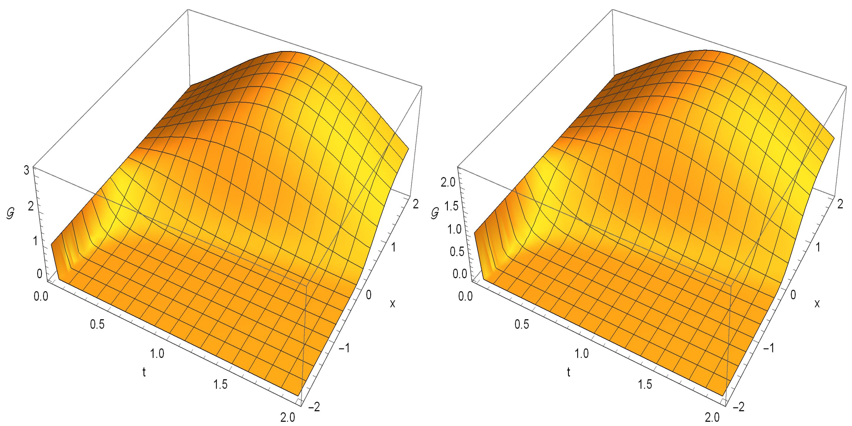
For $N=0,1,2,\dots ,$ the differential equation

$${\mathcal{G}}^{\left(N\right)}={\left({\displaystyle \frac{\partial }{\partial t}}\right)}^N\mathcal{G}(t,{\left[x\right]}_q|\lambda )=\left({\displaystyle \sum _{i=0}^N}{a}_i(N,{\left[x\right]}_q|\lambda )t^i\right)\mathcal{G}(t,{\left[x\right]}_q|\lambda )$$

has a solution

$$\mathcal{G}=\mathcal{G}(t,{\left[x\right]}_q|\lambda )={(1+\lambda )}^{{\displaystyle \frac{2{\left[x\right]}_{q}t-t^2}{\lambda }}}.$$

This is a plot of the surface for this solution.

In Figure 1 (left), we choose $-2\le x\le 2,q=1/10,\lambda =1/10,$ and $0\le t\le 2.$ In Figure 1 (right), we choose $-2\le x\le 2,q=1/10,\lambda =9/10,$ and $0\le t\le 2.$

Figure 1. Surface for the solution $\mathcal{G}(t,{\left[x\right]}_q|\lambda )$.

4. Zeros of the Degenerate $\mathbf{q}$-Hermite Polynomials

Recently, mathematicians have used software because it makes many concepts easier. These studies have allowed mathematicians to generate and visualize new ideas, to examine the properties of shapes, to create many conjectures. Based on this trend, we investigate the distribution and pattern of zeros of degenerate q-Hermite polynomials ${\mathcal{H}}_{n,q}\left(x\right|\lambda )$ according to the change of degree n in this section.

First, a few examples of the specific polynomials of ${\mathcal{H}}_{n,q}\left(x\right|\lambda )$ defined in Section 2 are shown below:

$$\begin{array}{l}{\mathcal{H}}_{0,q}\left(x\right|\lambda )=1,\\ {\mathcal{H}}_{1,q}\left(x\right|\lambda )={\displaystyle \frac{2log(1+\lambda )}{\lambda (1-q)}}-{\displaystyle \frac{2q^{x}log(1+\lambda )}{\lambda (1-q)}},\\ {\mathcal{H}}_{2,q}\left(x\right|\lambda )=-{\displaystyle \frac{2log(1+\lambda )}{\lambda }}+{\displaystyle \frac{4log{(1+\lambda )}^2}{{\lambda }^2{(1-q)}^2}}-{\displaystyle \frac{8q^{x}log{(1+\lambda )}^2}{{\lambda }^2{(1-q)}^2}}+{\displaystyle \frac{4q^{2x}log{(1+\lambda )}^2}{{\lambda }^2{(1-q)}^2}},\\ {\mathcal{H}}_{3,q}\left(x\right|\lambda )=-{\displaystyle \frac{12log{(1+\lambda )}^2}{{\lambda }^2(1-q)}}+{\displaystyle \frac{12q^{x}log{(1+\lambda )}^2}{{\lambda }^2(1-q)}}+{\displaystyle \frac{8log{(1+\lambda )}^3}{{\lambda }^3{(1-q)}^3}}-{\displaystyle \frac{24q^{x}log{(1+\lambda )}^3}{{\lambda }^3{(1-q)}^3}}\\ +{\displaystyle \frac{24q^{2x}log{(1+\lambda )}^3}{{\lambda }^3{(1-q)}^3}}-{\displaystyle \frac{8q^{3x}log{(1+\lambda )}^3}{{\lambda }^3{(1-q)}^3}}.\end{array}$$

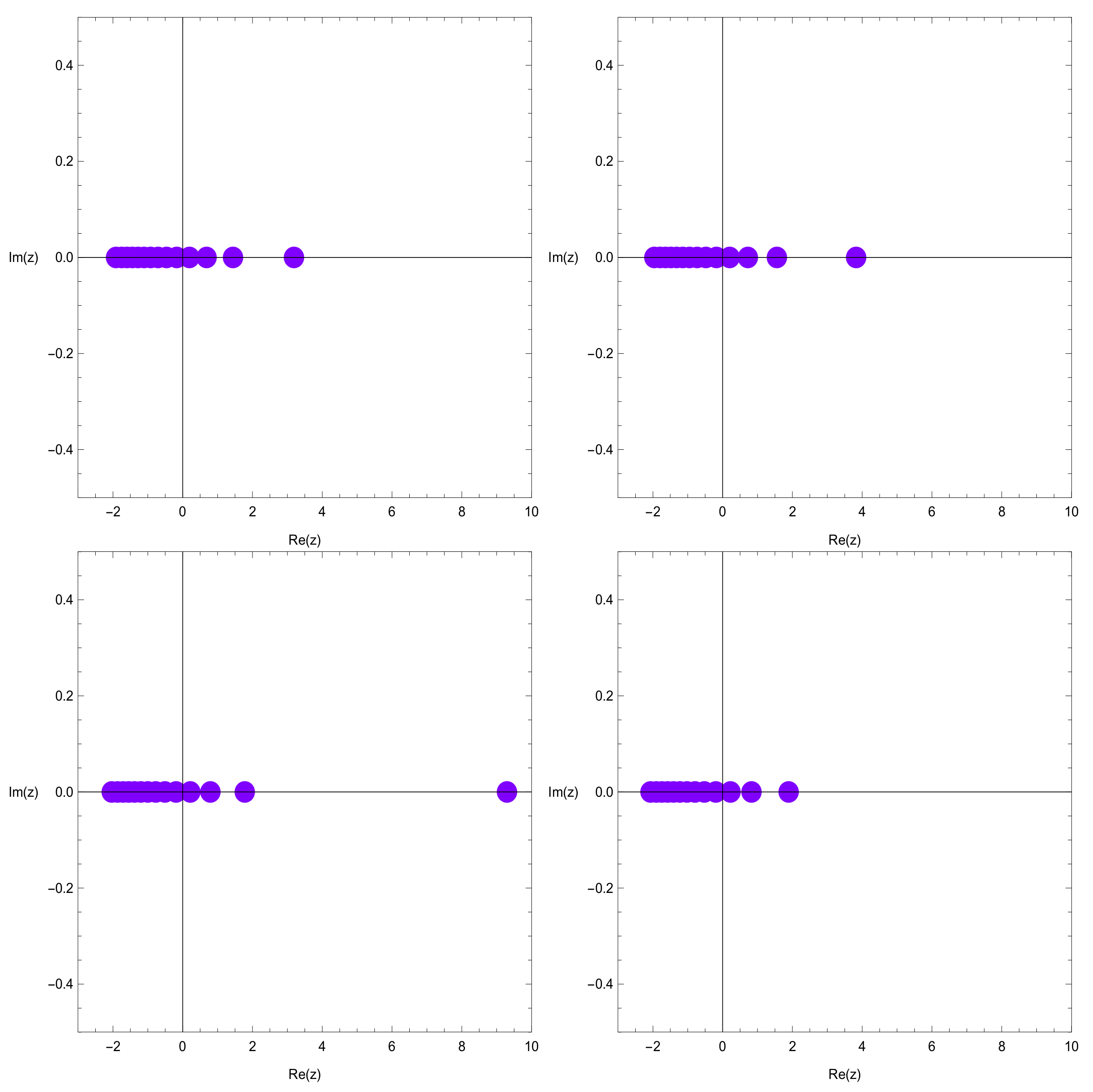
Using a computer, we investigate the distribution of zeros of the degenerate q-Hermite polynomials ${\mathcal{H}}_{n,q}\left(x\right|\lambda )=0$. Plots of the zeros of the degenerate q-Hermite polynomials ${\mathcal{H}}_{n,q}\left(x\right|\lambda )$ for $n=20$ and $x\in \mathbb{R}$ are as follows (Figure 2).

Figure 2. $\mathrm{Zeros} \mathrm{of} {\mathcal{H}}_{n,q}\left(x\right|\lambda )$.

In the top-left picture of Figure 2, we chose $n=20,q=1/10$ and $\lambda =1/10$. In the top-right picture of Figure 2, we chose $n=20,q=1/10$ and $\lambda =3/10$. In the bottom-left picture of Figure 2, we chose $n=20,q=1/10$ and $\lambda =7/10$. In the bottom-right picture of Figure 2, we chose $n=20,q=1/10$ and $\lambda =9/10$.

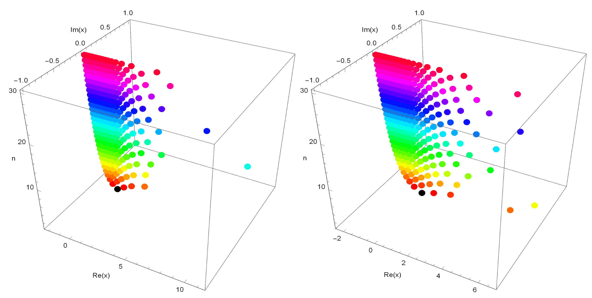
Stacks of zeros of the degenerate q-Hermite polynomials ${\mathcal{H}}_{n,q}\left(x\right|\lambda )$ for $1\le n\le 30$ from a 3-D structure are presented (Figure 3).

Figure 3. $\mathrm{Stacks} \mathrm{of} \mathrm{zeros} \mathrm{of} {\mathcal{H}}_{n,q}\left(x\right|\lambda ),1\le n\le 30$.

In the left picture of Figure 3, we chose $q=5/10$ and $\lambda =1/10$. In the right picture of Figure 3, we chose $q=5/10$ and $\lambda =9/10$.

Our numerical results for approximate solutions of real zeros of the degenerate q-Hermite polynomials ${\mathcal{H}}_{n,q}\left(x\right|\lambda ),q=1/2,\lambda =1/10,x\in \mathbb{R}$ are displayed (Table 1).

Table 1. Numbers of real and complex zeros of ${\mathcal{H}}_{n,q}\left(x\right|\lambda ),q=1/2,\lambda =1/10$.

Degree n	Real Zeros
1	1
2	2
3	3
4	4
5	4
6	5
7	6
8	6
9	7
10	8
11	8
12	9
13	10
14	10

We can see a regular pattern of the complex roots of the degenerate q-Hermite polynomials ${\mathcal{H}}_{n,q}\left(x\right|\lambda )=0$ and hope to verify the same kind of regular structure of the complex roots of the degenerate q-Hermite polynomials ${\mathcal{H}}_{n,q}\left(x\right|\lambda )=0$ (Table 1).

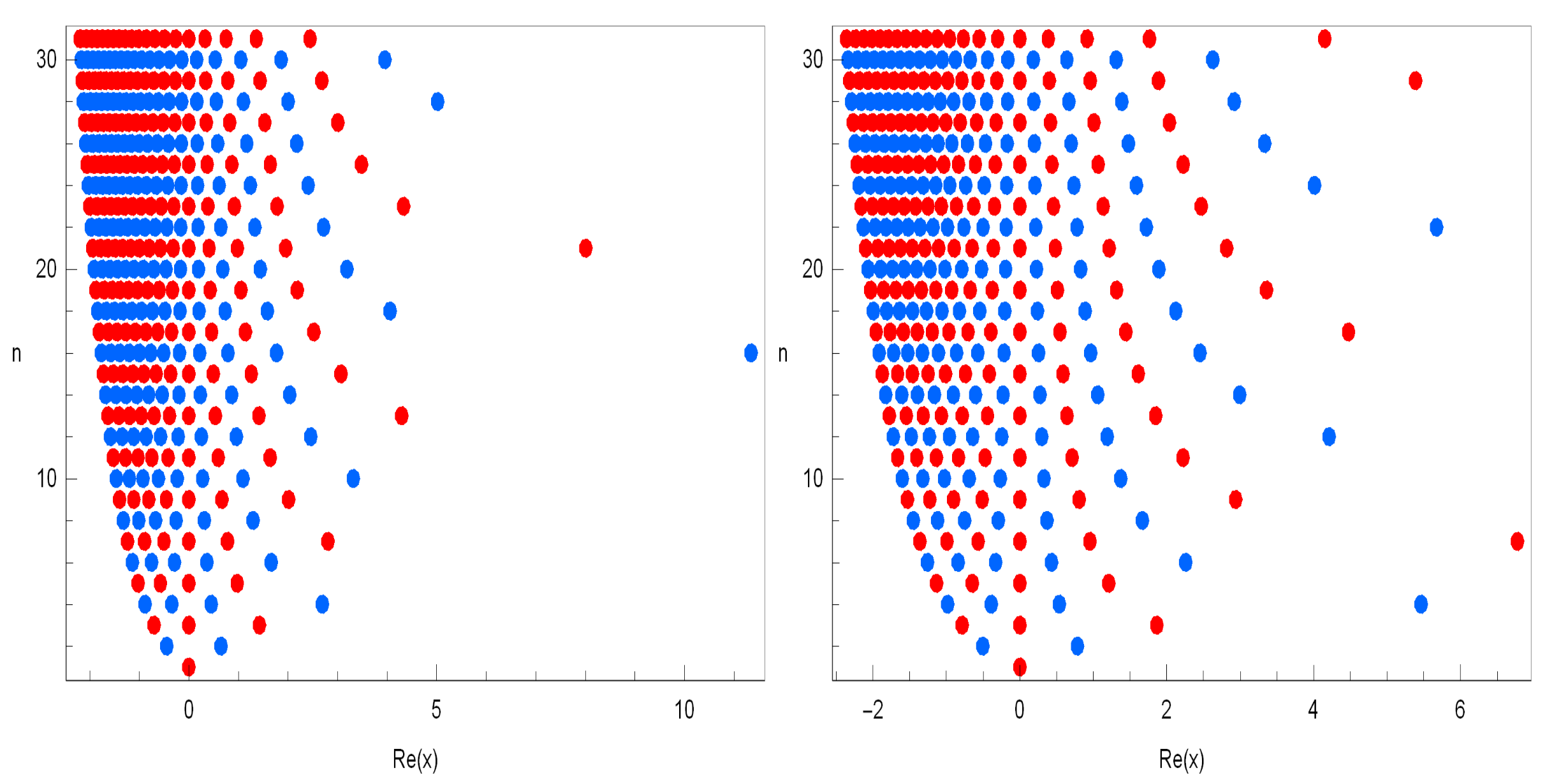
The plot of real zeros of the degenerate q-Hermite polynomials ${\mathcal{H}}_{n,q}\left(x\right|\lambda )$ for $q=1/2,1\le n\le 30$ structure are presented (Figure 4).

Figure 4. $\mathrm{Stacks} \mathrm{of} \mathrm{zeros} \mathrm{of} {\mathcal{H}}_{n,q}\left(x\right|\lambda ),1\le n\le 30$.

In the left picture of Figure 4, we chose $\lambda =1/10$. In the right picture of Figure 4, we chose $\lambda =9/10$.

Next, we calculated an approximate solution that satisfies ${\mathcal{H}}_{n,q}\left(x\right|\lambda )=0,q=1/2,\lambda =9/10,x\in \mathbb{R}$. The results are shown in Table 2.

Table 2. Approximate solutions of ${\mathcal{H}}_{n,q}\left(x\right|\lambda )=0,q=1/2,\lambda =9/10,x\in \mathbb{R}$.

Degree n	x
1	0
2	−0.504526,    0.782538
3	−0.786709,    0,    1.8632
4	−0.983545,    −0.390258,    0.536646,    5.46234
5	−1.13494,    −0.648504,    0,    1.20937
6	−1.25805,    −0.840698,    −0.331348,    0.430875,    2.25785
7	−1.36185,    −0.993392,    −0.56881,    0,    0.9526 ,    6.77359
8	−1.45162,    −1.11987,    −0.752868,    −0.293593
	0.369016,    1.66722

5. Conclusions

This paper focused on some explicit identities, recurrence relations and differential equations for c. Thus, we defined the degenerate q-Hermite polynomials ${\mathcal{H}}_{n,q}\left(x\right|\lambda )$ in Definition 1 and obtained their formulas (Theorem 1), including explicit formulae (Theorem 5 and Corollary 1) and differential equations (Theorems 2–4). Finally, we examined the distribution and pattern of zeros of degenerate q-Hermite polynomials ${\mathcal{H}}_{n,q}\left(x\right|\lambda )$ according to the change in degree n. We expect that research in this direction will be a new approach to using numerical methods for the study of degenerate q-Hermite polynomials ${\mathcal{H}}_{n,q}\left(x\right|\lambda )=0$.

References

1. Andrews, G.E.; Askey, R.; Roy, R. Special Functions; Cambridge University Press: Cambridge, UK, 1999. [Google Scholar]
2. Louisell, W.H. Quantum Statistical Properties of Radiation; Wiley: New York, NY, USA, 1973. [Google Scholar]
3. Dattoli, G.; Ottaviani, P.L.; Torre, A.; Vazquez, L. Evolution operator equations, integration with algebraic and finite difference methods: Applications to physical problems in classical and quantum mechanics. Riv. Nuovo Cimento 1997, 20, 1–133. [Google Scholar]
4. Haimo, D.T.; Markett, C. A representation theory for solutions of a higher-order heat equation II. J. Math. Anal. Appl. 1992, 168, 289–305. [Google Scholar] [CrossRef] [Green Version]
5. Andrews, L.C. Special Functions for Engineers and Mathematicians; Macmillan. Co.: New York, NY, USA, 1985. [Google Scholar]
6. Appell, P.; Hermitt, J. Fonctions Hyperge´ome´triques et Hypersphe´riques: Polynomes d Hermite; Gauthier-Villars: Paris, France, 1926. [Google Scholar]
7. Erdelyi, A.; Magnus, W.; Oberhettinger, F.; Tricomi, F.G. Higher Transcendental Functions; Krieger: New York, NY, USA, 1981; Volume 3. [Google Scholar]
8. Hwang, K.W.; Ryoo, C.S. Differential equations associated with two variable degenerate Hermite polynomials. Mathematics 2020, 8, 228. [Google Scholar] [CrossRef] [Green Version]
9. Riyasat, M.; Khan, S. Some results on q-Hermite based hybrid polynomials. Glas. Mat. 2018, 53, 9–31. [Google Scholar] [CrossRef]
10. Khan, S.; Nahid, T. Determinant Forms, Difference Equations and Zeros of the q-Hermite-Appell Polynomials. Mathematics 2018, 6, 258. [Google Scholar] [CrossRef] [Green Version]
11. Kim, T.; Choi, J.; Kim, Y.H.; Ryoo, C.S. On q-Bernstein and q-Hermite polynomials. Proceeding Jangjeon Math. Soc. 2011, 14, 215–221. [Google Scholar]
12. Ryoo, C.S.; Kang, J.Y. Some properties involving q-Hermite polynomials arising from differential equations and location of their zeros. Mathematics 2021, 7, 1168. [Google Scholar] [CrossRef]
13. Ryoo, C.S. Some identities involving the generalized polynomials of derangements arising from differential equation. J. Appl. Math. Inform. 2020, 38, 159–173. [Google Scholar]
14. Ryoo, C.S.; Agarwal, R.P.; Kang, J.Y. Differential equations associated with Bell-Carlitz polynomials and their zeros. Neural Parallel Sci. Comput. 2016, 24, 453–462. [Google Scholar]
15. Young, P.T. Degenerate Bernoulli polynomials, generalized factorial sums, and their applications. J. Number Theorey 2008, 128, 738–758. [Google Scholar] [CrossRef] [Green Version]
Publisher’s Note: MDPI stays neutral with regard to jurisdictional claims in published maps and institutional affiliations.
Article Metrics
Citations
Article Access Statistics
Multiple requests from the same IP address are counted as one view.