Sandstone Modeling under Axial Compression and Axisymmetric Lateral Pressure

Abstract

The problems of the mechanical state of rocks and other brittle materials are studied from different sides in a large number of publications, the flow of which does not weaken with time, which is explained by the relevance and complexity of these problems. Quantitative values of strength and other characteristics of such materials can be obtained experimentally or using numerical and analytical models. This work is aimed at developing an analytical model for analyzing the state of brittle material on the example of sandstone under axial compression and axisymmetric proportional lateral pressure. The research uses methods of modeling mechanical systems based on the basic ideas of fracture mechanics. For axial compression with proportional lateral pressure, the equation of the load–strain curve is obtained, and the functions of residual life and damage are justified; effective stresses and effective modulus of elasticity are determined; a calculation algorithm and examples of its application are given. The results of the simulation are consistent with the experimental data known from the literature. The results obtained to a certain extent clarify the understanding of the mechanism of rock damage and destruction under axial compression with lateral pressure.

1. Introduction

An analysis of the literature has shown that a large amount of research is focused on solving problems of analyzing the mechanical state of rocks and other brittle materials. The volume of research in this area does not decrease over time, which is explained by the relevance and complexity of the problems. Characteristics such as stresses, strains, damages and residual strength are necessary when designing new and predicting the condition of existing terrestrial and underground artificial and natural objects. Quantitative values of these characteristics for sandstone and other materials can be obtained experimentally; experimental data are needed not only to assess the technical condition of existing facilities, but are also used to test mathematical models designed to predict the state of brittle materials in natural objects and engineering structures, which is reflected in the reviews [1,2,3,4].

The standard way to obtain reliable strength characteristics of rocks, concrete and other brittle materials is a uniaxial compression test [5]. However, in real objects, brittle materials often function under conditions of triaxial loading, which is technically more difficult to reproduce in laboratory conditions. Nevertheless, these difficulties are gradually being overcome with the advent of new testing machines [6], and by now a fairly large array of experimental data on the behavior of sandstone and other rocks under triaxial loading has already been obtained. Progress in the field of experimental studies of brittle materials [7,8] has expanded the possibilities of verifying theoretical results and thereby stimulated the development of numerical, statistical and analytical mathematical models of the behavior of materials under various influences [9,10,11].

Numerical methods for modeling the behavior of brittle materials under load [8,12] are in a certain sense similar to the methods of testing real samples [7,8,13], since digital models and real tests allow obtaining data only for a discrete set of objects. When using numerical methods and computer technologies, there are practically no restrictions on the number and complexity of the objects under study, which makes it possible to study any of their states (albeit with a large expenditure of time and computer resources [14]), but a certain amount of experimental data is needed to verify the results of numerical modeling.

Statistical models, also called stochastic models, reflect the probabilistic nature of the interaction of material particles after the empirical selection of parameters of suitable distributions and their interpretation from a physical point of view. Many statistical models of the mechanical state of a brittle material are based on the use of the Weibull distribution [15] as a law postulating the law of damage accumulation [16]. It is known that a model of damage accumulation of brittle materials can be obtained without postulating the law of damage evolution; however, modeling in accordance with the logic of fracture mechanics leads to an equation [17] that corresponds to the Weibull distribution law, which confirms the fundamental importance and advantages of this law [18,19,20,21]. At the same time, in specific problems of fracture mechanics, certain limitations may arise in determining the coefficients of this distribution, which are overcome by clarifying the scope of its application [16].

Analytical models reflect, as a rule, the relationship between the fundamental physical and mechanical characteristics of a material not only in a certain set of its states but also with a continuous change in these characteristics over the entire range of values acceptable from a physical point of view, and therefore such models are an effective tool for predicting the behavior of brittle material under loading. However, it is hardly possible to build a fully analytical model of a complex object within the framework of applied research. Therefore, analytical and numerical methods are used together within the same model. For example, in the work of W.J. Drugan [22], two simple models of the fragmentation process of brittle material based on analytical mechanics were constructed; at the same time, this work was aimed both at obtaining an analytical result to the maximum extent possible and at minimizing the volume of numerical analysis. Thus, the use of analytical relations simplifies the mathematical description of the physical model and reduces the amount of calculations, and numerical methods provide sufficient versatility of the model.

The current work is aimed at developing a fully analytical model of the behavior of brittle material under axial compression and proportional axisymmetric lateral pressure. In addition, it was assumed to use only the necessary and sufficient initial data, which are the main characteristics of brittle materials for which there is an extremum point on the load–displacement curve. Thus, the scope of the model is limited, but it covers materials such as sandstone, marble, concrete and some other similar materials. Modeling of the load–displacement dependence in this paper is carried out by generalizing the well-known approach, which was theoretically justified only for uniaxial compression [17,23], as well as taking into account the results of studies of various aspects of the problem from articles by other authors [24,25,26].

The new results obtained in this work include the following: for axial compression with proportional lateral pressure, the equation of the full curve of the load dependence on strain is obtained; the functions of residual life and damage are justified; effective stresses and effective modulus of elasticity are determined; and a calculation algorithm is given and examples of its application are analyzed. The model was tested using experimental data known from the literature for sandstone. Taking into account the lateral pressure complicates the stage of model justification; since not all problems have been solved, the scope of the model and algorithm is limited to axial compression at proportional lateral pressure without taking into account time and strain rate. However, the result in the form of analytical relations opens up some new opportunities for continuing applied research on the behavior of brittle materials under loading.

2. Methodology

2.1. Compression of Brittle Material with Proportional Lateral Pressure

By analogy with [17], we assume that a brittle material consists of particles that differ in size, shape, strength of the particle material and the strength of the bonds between the particles. The Young’s modulus of the material of all particles is the same and is equal to some average value of $E$. With a sufficiently large load, the particles and the bonds between them are not destroyed simultaneously. If the strain increase, then the weakest particle from the number of intact particles is first destroyed and detached, which step by step reduces the cross-sectional area of the sample from the initial value $A_0$ to some value $\tilde{A}$. The value $\tilde{A}$ is called the effective cross-sectional area [27]. Since the cross-sectional area of the sample decreases with increasing strain, the stiffness of the sample also decreases. For the same reason (reducing the area from $A_0$ to $\tilde{A}$), the bearing capacity of the sample decreases.

Thus, damage to a brittle material during its loading is modeled by an ordered set of discrete states and stages, at each of which the weakest particle of the number of particles remaining intact is destroyed. Accordingly, the effective area $\tilde{A}$ gradually decreases. It is logical to assume that the decrease in area $\tilde{A}$ at each step is proportional to the change in the energy of elastic strain. The adequacy of this assumption is confirmed by the consistency of the simulation results with experiments known in the literature when solving problems of statics and kinematics of uniaxial compression of brittle material without lateral pressure [23]. Consider the application of this (energy) approach to the analysis of brittle material under compression with proportional lateral pressure (Figure 1a). A typical load–displacement plot for such cases is shown in Figure 1b, which also shows the geometric value of the tangent ($E$) and secant ($E_{secant}$) modulus of elasticity. These modules can also be formally defined for other points of the plot; however, the interpretation shown in Figure 1b is used from here on forward.

Let’s use Hooke’s law (1):

$$\begin{gathered} {\epsilon }_1=\left(1/E\right)\left({\sigma }_1-\nu \left({\sigma }_2+{\sigma }_3\right)\right) \\ {\epsilon }_2=\left(1/E\right)({\sigma }_2-\nu \left({\sigma }_3+{\sigma }_1\right)) \\ {\epsilon }_3=\left(1/E\right)({\sigma }_3-\nu \left({\sigma }_1+{\sigma }_2\right)) \end{gathered}$$

(1)

From the first relation (1) we express ${\sigma }_1$ and taking into account the equalities ${\sigma }_2={\sigma }_3=k{\sigma }_1$ (Figure 1a) we write:

$$\begin{gathered} {\sigma }_1=\frac{{\epsilon }_{1}E}{1-2\nu k} \\ {\sigma }_2={\sigma }_3=\frac{k{\epsilon }_{1}E}{1-2\nu k} \end{gathered}$$

(2)

Using the relations in (2), we represent ${\epsilon }_2$ and ${\epsilon }_3$ in the following form:

$${\epsilon }_2={\epsilon }_3={\epsilon }_1\frac{k-\nu \left(k+1\right)}{1-2\nu k}$$

The elastic strain energy for a unit volume is determined by analogy with [28]:

$$w=\frac{1}{2E}\left({\sigma }_1^2+{\sigma }_2^2+{\sigma }_3^2-2\nu \left({\sigma }_1{\sigma }_2+{\sigma }_2{\sigma }_3+{\sigma }_3{\sigma }_1\right)\right)$$

(3)

Taking into account the relations in (2), we transform Equation (3) to form (4):

$$w=\frac{1}{2}{\epsilon }_1^{2}E\frac{1+2k^2-2\nu k\left(2+k\right)}{{\left(1-2\nu k\right)}^2}$$

(4)

For the compactness of the formulas, the complex of coefficients $\nu$ and $k$ in relation (4) is denoted as the parameter ${\mu }^{\left(k\right)}$ (5); then we can rewrite (4) to form (6):

$${\mu }^{\left(k\right)}=\frac{1+2k^2-2\nu k\left(2+k\right)}{{\left(1-2\nu k\right)}^2}$$

(5)

$$w=\frac{1}{2}{\epsilon }_1^{2}E{\mu }^{\left(k\right)}$$

(6)

2.2. Residual Resource Function, Effective Area and Damage Function

Concretizing the presentation of the research material, let us consider a sample of brittle material in the form of a cylinder, the height and cross-sectional area of which in the undeformed state are, respectively, $H_0$ and $A_0$. During loading, the sample is deformed. If the axial strain changes from ${\epsilon }_1$ to ${\epsilon }_1+d{\epsilon }_1$, then the effective cross-sectional area $\tilde{A}$ decreases by a certain amount of $d\tilde{A}$. In this case, the change in the height of the sample and its volume is equal, respectively, to $dH=H_{0}d{\epsilon }_1$ and $dV=\tilde{A}dH=\tilde{A}{H}_{0}d{\epsilon }_1$. The elastic strain energy per unit volume is determined by the ratio (6). Then, if the volume change is $dV$, then the change in the elastic strain energy is $dW=wdV=w\tilde{A}{H}_{0}d{\epsilon }_1$. Let us rewrite this equation using (6):

$$dW=\frac{1}{2}{\epsilon }_1^{2}E{\mu }^{\left(k\right)}\tilde{A}{H}_{0}d{\epsilon }_1$$

(7)

We assume that the change in the effective area ($d\tilde{A}$) is proportional to the change in the elastic strain energy $dW$ (7) with a certain proportionality coefficient $\beta$:

$$d\tilde{A}=-\beta dW=-\beta \frac{1}{2}{\epsilon }_1^{2}E{\mu }^{\left(k\right)}\tilde{A}{H}_{0}d{\epsilon }_1$$

(8)

The minus sign means that if the strain ${\epsilon }_1$ increases, then the effective cross-sectional area ($\tilde{A}$) decreases. In the model under consideration, the modulus of elasticity, as noted above, is the same for all particles and equal to some average value and does not change during loading. The proportionality coefficient $\beta$ is constant within the framework of solving a specific problem. Let

$$\beta =\frac{2}{{({\epsilon }_{1, extr}^{test})}^{3}E{H}_0}$$

(9)

The value of ${\epsilon }_{1, extr}^{test}$ is determined experimentally and corresponds to the extremum point of the function ${\sigma }_1\left({\epsilon }_1\right)$ (Figure 1b). Examples of experimental graphs of stress ${\sigma }_1$ as a function of strain ${\epsilon }_1$ during compression of sandstone samples with confining lateral pressure can be found in [13]

Using the Equation (9), we rewrite (8) to form (10):

$$d\tilde{A}=-\frac{{\mu }^{\left(k\right)}}{{({\epsilon }_{1, extr}^{test})}^3}\tilde{A}{\epsilon }_1^{2}d{\epsilon }_1$$

(10)

Dividing both parts of equality (10) by $A_0$ and denote $\theta =\tilde{A}/A_0$. Then this equation can be rewritten as (11):

$$\frac{d\theta }{\theta }=-\frac{{\mu }^{\left(k\right)}}{{({\epsilon }_{1, extr}^{test})}^3}{\epsilon }_1^{2}d{\epsilon }_1$$

(11)

We integrate Equation (11), taking into account that if ${\epsilon }_1=0$, then $\tilde{A}=A_0$ and $\theta =1$:

$$\theta =e^{-\frac{{\mu }^{\left(k\right)}}{3}{\left(\frac{{\epsilon }_1}{{\epsilon }_{1, extr}^{test}}\right)}^3}$$

(12)

If ${\epsilon }_1={\epsilon }_{1, extr}^{test}$, then $\theta ={\theta }_{extr}=e^{-{\mu }^{\left(k\right)}/3}$.

In the physical sense, the function $\theta =\tilde{A}/A_0$, where $0\le \tilde{A}\le$_0, determines the proportion of undamaged particles; i.e., the residual bearing capacity of the sample. Accordingly, Function (12) is the residual resource function.

Since $\theta =\tilde{A}/A_0$, then by using the ratio in (12) we can determine the effective cross-sectional area of the sample:

$$\tilde{A}=A_0{e}^{-\frac{{\mu }^{\left(k\right)}}{3}{\left(\frac{{\epsilon }_1}{{\epsilon }_{1, extr}^{test}}\right)}^3}$$

(13)

Since Function (12) determines the proportion of undamaged disturbed particles, the proportion of destroyed particles is equal to $D=1-\theta$. Thus, the damage function $D$ can be written as (14):

$$D=1-\theta$$

(14)

2.3. Determination of the Effective Modulus of Elasticity

We will rewrite the relations in (2) in terms of effective stresses:

$$\begin{gathered} {\tilde{\sigma }}_1=\frac{{\epsilon }_1\tilde{E}}{1-2\nu k} \\ {\tilde{\sigma }}_2={\tilde{\sigma }}_3=\frac{k{\epsilon }_1\tilde{E}}{1-2\nu k} \end{gathered}$$

(15)

From the first equation in (15), we express $\tilde{E}$ and, taking into account the relation (12), we obtain:

$$\tilde{E}=\frac{{\tilde{\sigma }}_1}{{\epsilon }_1}\left(1-2\nu k\right)=\frac{{\sigma }_1}{{\epsilon }_1\theta }\left(1-2\nu k\right)$$

(16)

The equations in (16) are defined for any values of ${\epsilon }_1$ corresponding to the physical meaning of the problem. Let ${\epsilon }_1={\epsilon }_{1, extr}^{test}$ and, respectively, ${\sigma }_1={\sigma }_{1, extr}^{test}$ (Figure 1b). Then, the equations in (16) can be written as:

$$\tilde{E}=\frac{{\sigma }_1}{{\epsilon }_1\theta }\left(1-2\nu k\right)=\frac{{\sigma }_{1, extr}^{test}}{{\epsilon }_{1, extr}^{test}{\theta }_{extr}}\left(1-2\nu k\right)=\frac{E_{secant}}{{\theta }_{extr}}\left(1-2\nu k\right).$$

(17)

As noted above, we assume that in the model under consideration, the effective modulus of elasticity ($\tilde{E}$), as a physical characteristic of the material, does not depend on the method of its determination. This means that the value of $\tilde{E}$ can be determined by the results of standard tests for uniaxial compression, which is modeled using the ratios in (5) and (17) if $k=0$; in this case, ${\mu }^{\left(k\right)}=1$. Thus,

$$\tilde{E}=E_{secant}{e}^{1/3}\approx 1.396E_{secant}$$

(18)

An analogue of Relation (18) was obtained in [17].

In the ratios in (17) and (18), the secant modulus of elasticity is used (Figure 1b), which is defined as

$$E_{secant}=\frac{{\sigma }_{1, extr}^{test}}{{\epsilon }_{1, extr}^{test}}$$

(19)

Commenting on Relations (18) and (19), we note the following. From the standpoint of geometry, the secant modulus of elasticity can be defined as the tangent of the angle of inclination of a straight line that connects the origin with any point on the graph of the function ${\sigma }_1\left({\epsilon }_1\right)$. However, the developed model uses a straight line that connects the origin, shifted to point $B$, with the extremum point (Figure 1b). From a physical point of view, the preference for such a choice is explained by the fact that the values of ${\epsilon }_{1, extr}^{test}$ and ${\sigma }_{1, extr}^{test}$ corresponds to only one point on the graph of the function ${\sigma }_1\left({\epsilon }_1\right)$.

In addition, the values of ${\epsilon }_{1, extr}^{test}$ and ${\sigma }_{1, extr}^{test}$ depend on all factors that explicitly or latently affect the results of the experiment (Figure 1b), and, therefore, these factors are directly or indirectly integrally taken into account in these two values. Hence, this pair of values (${\epsilon }_{1, extr}^{test}$ and ${\sigma }_{1, extr}^{test}$) can be considered as a characteristic of the physical properties of a brittle material under axial compression with lateral proportional pressure. If this statement is true, then points with experimentally determined coordinates ${\epsilon }_{1, extr}^{test}$ and ${\sigma }_{1, extr}^{test}$ will be localized on a straight line whose equation ${\sigma }_1=E_{secant}{\epsilon }_1$, where $E_{secant}={\sigma }_{1, extr}^{test}/{\epsilon }_{1, extr}^{test}$. Validation of this assumption is performed in Section 3.3.

2.4. Effective Stress

Combining Equation (15) and $\tilde{E}={\sigma }_1\left(1-2\nu k\right)/\left({\epsilon }_1\theta \right)$ from Equation (16), we obtain:

$${\tilde{\sigma }}_1=\frac{{\sigma }_1}{\theta }$$

(20)

$${\tilde{\sigma }}_2={\tilde{\sigma }}_3=k\frac{{\sigma }_1}{\theta }$$

(21)

If the compression is uniaxial, then $k=0$ (Figure 1) and ${\mu }^{\left(k\right)}=1$ (5); then using (20) and (12), we get

$${\tilde{\sigma }}_{1,u}=\frac{{\sigma }_1}{\theta }={\sigma }_1{e}^{ \frac{1}{3}{\left(\frac{{\epsilon }_1}{{\epsilon }_{1, extr}^{test}}\right)}^3}$$

(22)

An analogue of the ratio in (22) for uniaxial compression was obtained in [17].

Let us pay attention to the fact that both the function ${\sigma }_1\left({\epsilon }_1\right)$, a typical graph of which is shown in Figure 1b, and the residual resource function $\theta$ (12) in the ratios in (21) and (22) depend non-linearly on the strain of ${\epsilon }_1$, but this nonlinearity does not mean that the effective stress (20) is also a non-linear function.

2.5. Residual Resource Function, Effective Modulus of Elasticity and Apparent Modulus of Elasticity

There are some difficulties on the way to the experimental determination of the effective characteristics of the material that degrades during compression. At the same time, it is relatively simple to determine the apparent stresses and elastic modulus of the material (Figure 1b). Therefore, the relations between effective and apparent characteristics in fracture mechanics are formulated at the level of hypotheses; for example, the hypothesis of equivalent strain is used [12].

Using the residual resource function (12) justified above, the ratio between the effective stress (${\tilde{\sigma }}_1$), the effective modulus of elasticity ($\tilde{E}$), the apparent stress (${\sigma }_1$) and the apparent modulus of elasticity ($E$) can be found.

Let the apparent stress ${\sigma }_1$ and the effective stress ${\tilde{\sigma }}_1$ be found for a certain value ${\epsilon }_1$. Using Equations (2) and (15), we write, respectively, ${\epsilon }_1={\sigma }_1\left(1-2\nu k\right)/E$ and ${\epsilon }_1={\tilde{\sigma }}_1\left(1-2\nu k\right)/\tilde{E}$. It follows from these equalities that the effective (${\tilde{\sigma }}_1 и \tilde{E})$ and apparent (${\sigma }_1$ and $E)$ characteristics are related by the following relation, which is based on the aforementioned hypothesis of equivalence of deformations [12]:

$$\frac{{\sigma }_1}{E}=\frac{{\tilde{\sigma }}_1}{\tilde{E}}$$

(23)

If in Equation (23) ${\tilde{\sigma }}_1={\sigma }_1/\theta$ (20), then, taking into account (14), we write:

$$\tilde{E}=\frac{E}{\theta }=\frac{E}{1-D}$$

(24)

In the model under consideration, the tangent (aka apparent) modulus of elasticity ($E$) and the residual resource function $\theta$ (12) are nonlinear strain functions ${\epsilon }_1$. Since $\theta \le 1$, the elastic modulus $\tilde{E}$ and $E$, according to (24), are related as $\tilde{E}\ge E$.

2.6. Equation of the Stress–Strain Curve under Axial Compression with Proportional Lateral Pressure

The purpose of this section is to substantiate the equation of the stress–strain curve and determine the effective stresses for the sample in Figure 1a. In the case under consideration, ${\sigma }_2={\sigma }_3=k{\sigma }_1$; these equations, as well as the relations in (2), can be written in terms of effective stresses: ${\tilde{\sigma }}_2={\tilde{\sigma }}_3=k{\tilde{\sigma }}_1$, гдe ${\tilde{\sigma }}_1={\epsilon }_1\tilde{E}/\left(1-2\nu k\right)$. Using these and Equation (12), we can write:

$$\tilde{E}=\frac{{\tilde{\sigma }}_1}{{\epsilon }_1}\left(1-2\nu k\right)=\frac{{\sigma }_1}{{\epsilon }_1\theta }\left(1-2\nu k\right)=\frac{{\sigma }_1}{{\epsilon }_1}\left(1-2\nu k\right)e^{ \frac{{\mu }^{\left(k\right)}}{3}{\left(\frac{{\epsilon }_1}{{\epsilon }_{1, extr}^{test}}\right)}^3}$$

(25)

The equations in (25) are defined for all values of ${\epsilon }_1$ and ${\sigma }_1$ corresponding to the physical meaning of the problem; for example, if ${\epsilon }_1={\epsilon }_{1,extr}^{test}$ and ${\sigma }_1={\sigma }_{1,extr}^{test}$, then

$$\tilde{E}=\frac{{\sigma }_{1,extr}^{test}}{{\epsilon }_{1,extr}^{test}}\left(1-2\nu k\right)e^{ \frac{{\mu }^{\left(k\right)}}{3}}$$

(26)

The left-hand side of Equations (25) and (26) are the same. From the condition of equality of the right parts of the same equations, we express the stress ${\sigma }_1$, which we denote as ${\sigma }_1^{*}$:

$${\sigma }_1^{\ast }={\sigma }_{1,extr}^{test}\frac{{\epsilon }_1}{{\epsilon }_{1,extr}^{test}}{e}^{ \frac{{\mu }^{\left(k\right)}}{3}(1-{\left(\frac{{\epsilon }_1}{{\epsilon }_{1, extr}^{test}}\right)}^3)}$$

(27)

As noted above, in the model under consideration, it is assumed that Function (27) has an extremum (Figure 1b). The peak point must correspond to the value $\epsilon ={\epsilon }_{1,extr}^{test}$. Equation (27) does not correspond to this condition; therefore, its correction is necessary. Using condition $\epsilon ={\epsilon }_{1,extr}^{test}$ it can be found that the fraction ${\epsilon }_1/{\epsilon }_{1, extr}^{test}$ must be supplemented with a multiplier of ${\mu }^{\left(k\right)}{}^{-1/3}$; that is, instead of Equation (27), the following Equation (28) should be used, which corresponds to the condition $d{\sigma }_1/d{\epsilon }_1=0$:

$${\sigma }_1=\frac{{\epsilon }_1 {\sigma }_{1,extr}^{test}}{{\mu }^{{\left(k\right)}^{1/3}} {\epsilon }_{1,extr}^{test}}{e}^{ \frac{{\mu }^{\left(k\right)}}{3}(1-{\left(\frac{{\epsilon }_1}{{\mu }^{{\left(k\right)}^{1/3}}{\epsilon }_{1, extr}^{test}}\right)}^3)}={\epsilon }_1\frac{E_{secant}}{{\mu }^{{\left(k\right)}^{1/3}}}{e}^{ \frac{1}{3} ( {\mu }^{\left(k\right)}-{\left(\frac{{\epsilon }_1}{{\epsilon }_{1, extr}^{test}}\right)}^3)}$$

(28)

Check: using the ratio (28), we find:

$$d{\sigma }_1/d{\epsilon }_1=\frac{{\sigma }_{1,extr}^{test}}{{\mu }^{{\left(k\right)}^{\frac{1}{3}}} {({\epsilon }_{1,extr}^{test})}^4}{e}^{ \frac{{\mu }^{\left(k\right)}}{3}(1-{\left(\frac{{\epsilon }_1}{{\mu }^{{\left(k\right)}^{\frac{1}{3}}} {\epsilon }_{1, extr}^{test}}\right)}^3)}({\left({\epsilon }_{1,extr}^{test}\right)}^3-{\epsilon }_1^3).$$

(29)

It follows from (29) that the above condition $d{\sigma }_1/d{\epsilon }_1=0$ is executed if ${\epsilon }_1={\epsilon }_{1,extr}^{test}$. Therefore, next we will use Equation (28). Accordingly, the residual resource function $\theta$ should also be adjusted, i.e., instead of the ratio in (12), the Equation (30) should be used:

$$\theta =e^{-\frac{{\mu }^{\left(k\right)}}{3}{\left(\frac{{\epsilon }_1}{{\mu }^{{\left(k\right)}^{\frac{1}{3}}} {\epsilon }_{1, extr}^{test}}\right)}^3}=e^{-\frac{1}{3} {\left(\frac{{\epsilon }_1}{ {\epsilon }_{1, extr}^{test}}\right)}^3}$$

(30)

Function (30) should be used instead of Relation (14) when determining the damage function $D=1-\theta$:

$$D=1-\theta =1-e^{-\frac{1}{3} {\left(\frac{{\epsilon }_1}{ {\epsilon }_{1, extr}^{test}}\right)}^3}$$

(31)

The damage function (31) clearly does not depend on the parameter ${\mu }^{\left(k\right)}$; i.e., the form of the function is the same for both uniaxial compression with lateral pressure ($k\ne 0$, Figure 1a) and uniaxial compression without lateral pressure ($k=0$, ${\mu }^{\left(k\right)}=1$ (5)). However, this does not mean that the functions $\theta$ (30) and $D$ (31) do not depend on the properties of the material, since these functions depend on the strain ${\epsilon }_{1,extr}^{test}$ corresponding to the peak stress value (${\sigma }_{1,extr}^{test}$), and the values of ${\epsilon }_{1,extr}^{test}$ and ${\sigma }_{1,extr}^{test}$ is uniquely determined by the physical properties of the material and the load, which follows from Relations (5) and (28). At the same time, if ${\epsilon }_1={\epsilon }_{1,extr}^{test}$, then $\theta =e^{-1/3}\approx 0.72$ and $D=0.28$. Examples of calculating functions $\theta$ (30) и $D$ (31) are given in Section 3.2 and Section 4.1.

An analogue of the residual resource function (30), but only for uniaxial compression, was considered in the articles [23,30].

So, using the ratios in (20), (28) and (30), we determine the effective compression stress with lateral pressure for the sample according to Figure 1a:

$${\tilde{\sigma }}_1=\frac{{\sigma }_1}{\theta }={\epsilon }_1\frac{E_{secant}}{{\mu }^{{\left(k\right)}^{1/3}}} e^{{\mu }^{\left(k\right)}/3 }$$

(32)

The parameter ${\mu }^{\left(k\right)}$ simulates the effect of the Poisson ratio and lateral pressure.

In the simplest case, if the compression is uniaxial (without lateral pressure), then $k=0$ (Figure 1a), ${\mu }^{\left(k\right)}=1$; since $E_{secant} e^{1/3 }=\tilde{E}$, then in this particular case ${\tilde{\sigma }}_1={\epsilon }_1{E}_{secant} e^{1/3 }={\epsilon }_1\tilde{E}$.

To use the obtained relations for practical calculations, we systematize them in the form of an algorithm (Section 3.1).

3. Results Modeling and Comparison with Experiments Known in the Literature

3.1. Algorithm

The calculation algorithm based on the above relations can be written in the following form (

Table 1. Calculation algorithm.

Step Number	What Is Calculated in a Step 2, …, 8	Equations	Equations Label
1	We form the initial data: $\nu$$, {\sigma }_{1,extr}^{test}$$, {\epsilon }_{1,extr}^{test}$$, {\sigma }_{conf}$. We determine the coefficient of proportionality $k$ (Figure 1). Using this data, we perform the calculations indicated in the following paragraphs 2,…, 8.
2	Parameter ${\mu }^{\left(k\right)}$	${\mu }^{\left(k\right)}=\frac{1+2k^2-2\nu k\left(2+k\right)}{{\left(1-2\nu k\right)}^2}$	(5)
3	Secant modulus of elasticity	$E_{secant}=\frac{{\sigma }_{1, extr}^{test}}{{\epsilon }_{1, extr}^{test}}$	(19)
4	Effective modulus of elasticity	$\tilde{E}=E_{secant}{e}^{\frac{1}{3}}\approx 1.396E_{secant}$	(18)
5	Residual resource function	$\theta =e^{-\frac{1}{3} {\left(\frac{{\epsilon }_1}{ {\epsilon }_{1, extr}^{test}}\right)}^3}$	(30)
6	Damage function	$D=1-\theta$	(31)
7	Apparent stress	${\sigma }_1={\epsilon }_1\frac{E_{secant}}{{\mu }^{\left(k\right)}{}^{1/3}}{e}^{ \frac{1}{3 } ({\mu }^{\left(k\right)}-{\left(\frac{{\epsilon }_1}{{\epsilon }_{1, extr}^{test}}\right)}^3)}$	(28)
8	Effective stress	${\tilde{\sigma }}_1=\frac{{\sigma }_1}{\theta }$	(32)

).

An example of the application of the algorithm will be considered in the following subsection.

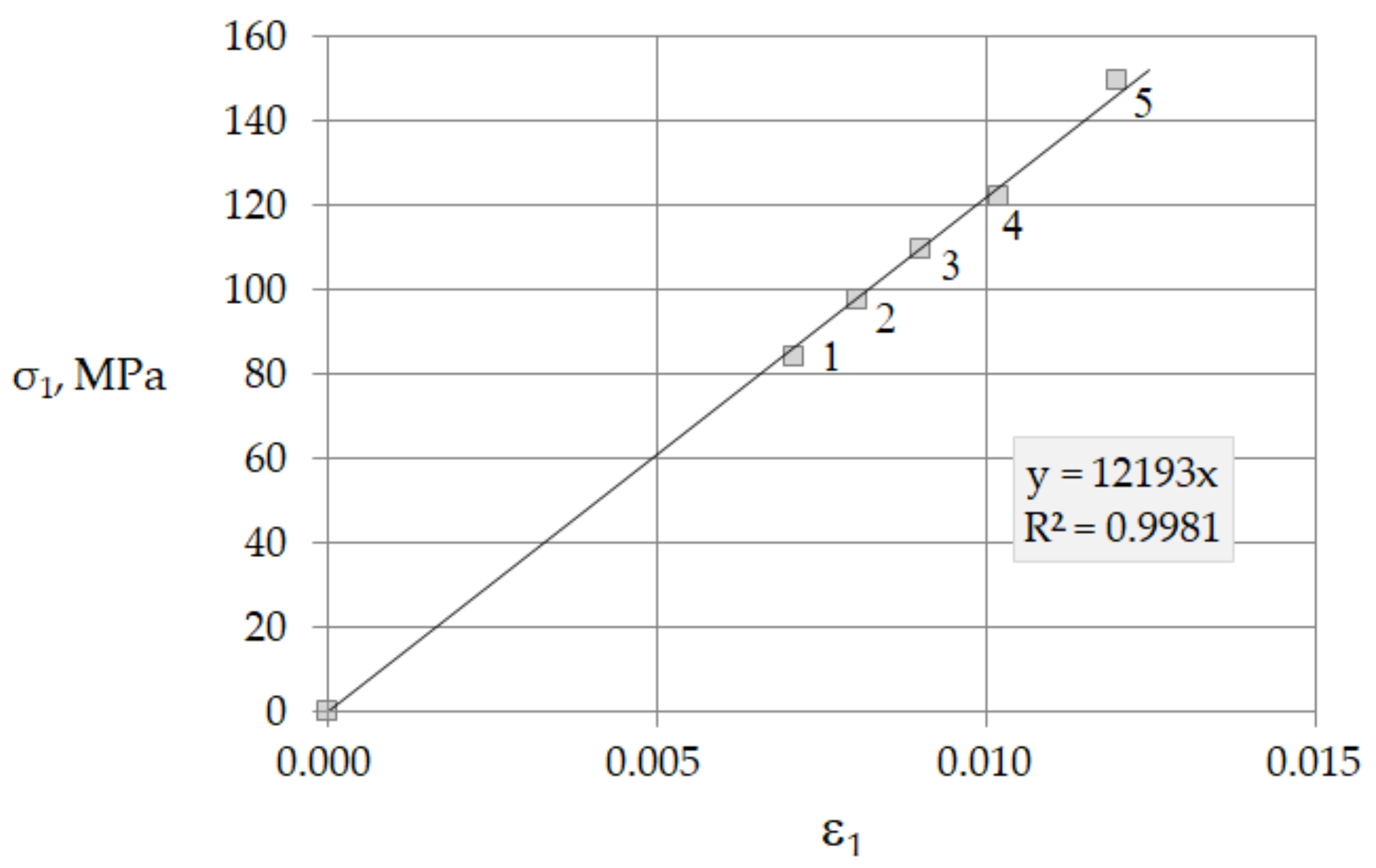
3.2. Example 1: Sandstone

To form the initial data, we used the results of testing sandstone published in the article P.Y. Hou et al. [7]. Namely, the values of Poisson’s ratio after the cited work [7] were used; ${\sigma }_{1,extr}^{test}$, ${\epsilon }_{1,extr}^{test}$ and ${\sigma }_{conf}$ were determined using the (${\sigma }_1-{\sigma }_3)$ vs. ${\epsilon }_1$ of the tested sandstone under uniaxial and tri-axial compressions by axial-strain-controlled loading plots from the same paper [7]. To obtain the values ${\sigma }_{1,extr}^{test}$, the ordinates of the plots (${\sigma }_1-{\sigma }_3)$ vs. ${\epsilon }_1$ from the cited article were recalculated to obtain the dependences ${\sigma }_1$ vs. ${\epsilon }_1$. The ${\epsilon }_1$ values were recalculated to account for vertical axis offset, as shown in Figure 1b. The initial data obtained in this way and some results of the calculations according to the algorithm from Section 3.1 are shown in

Table 2. Initial data and calculation results for sandstone.

Sample Number	Poisson’s Ratio ν	${\mathit{\sigma }}_{\mathit{c}\mathit{o}\mathit{n}\mathit{f}}$ (MPa)	Axial Stress Peak $({\mathit{\sigma }}_{1,\mathit{e}\mathit{x}\mathit{t}\mathit{r}}^{\mathit{t}\mathit{e}\mathit{s}\mathit{t}})$ (MPa)	$\mathit{k}$ $\left(\frac{{\mathit{\sigma }}_{\mathit{c}\mathit{o}\mathit{n}\mathit{f}}}{{\mathit{\sigma }}_{1,\mathit{e}\mathit{x}\mathit{t}\mathit{r}}^{\mathit{t}\mathit{e}\mathit{s}\mathit{t}}}\right)$	${\mathit{\mu }}^{\left(\mathit{k}\right)}$	Axial Strain at the Peak $({\mathit{\epsilon }}_{1,\mathit{e}\mathit{x}\mathit{t}\mathit{r}}^{\mathit{t}\mathit{e}\mathit{s}\mathit{t}})$	${\mathit{E}}_{\mathit{s}\mathit{e}\mathit{c}\mathit{a}\mathit{n}\mathit{t}}$ $\left(\frac{{\mathit{\sigma }}_{1,\mathit{e}\mathit{x}\mathit{t}\mathit{r}}^{\mathit{t}\mathit{e}\mathit{s}\mathit{t}}}{{\mathit{\epsilon }}_{1,\mathit{e}\mathit{x}\mathit{t}\mathit{r}}^{\mathit{t}\mathit{e}\mathit{s}\mathit{t}}}\right)$ (MPa)	$\tilde{\mathit{E}}$ (MPa)
1	0.17	0.00	84.03	0.0000	1.0000	0.00708	11,868	16,569
2	0.20	1.00	97.60	0.0102	1.0002	0.00804	12,139	16,946
3	0.21	2.50	109.5	0.0230	1.0007	0.00901	12,153	16,965
4	0.22	5.00	122.2	0.0409	1.0024	0.0102	11,980	16,724
5	0.22	10.00	149.7	0.0668	1.0062	0.0119	12,559	17,532

.

It should be noted that the above relationships (Section 3.1) are obtained under the assumption that the stress ${\sigma }_3={\sigma }_{conf}$ changes during loading in proportion to the axial load (Figure 1a). Therefore, comparison with tests at a constant value of ${\sigma }_{conf}$ is not entirely correct. We have not been able to find more suitable experimental data. Nevertheless, the comparison under consideration is expedient, because it contributes to a better understanding of the problem raised, which will clarify the direction of further research in the interests of engineering practice.

The results of the calculations according to the algorithm (Section 3.1) are presented graphically in Figure 2. The theoretical dependences of apparent values (${\sigma }_1$) on strain (${\epsilon }_1$) (Formula (28)) are shown by curves 1,…, 5; peak values ${\sigma }_1$ denoted by markers in the form of squares. The asterisks mark the points at which the accelerated destruction in the post-peak state begins. The slope angles of the solid and dotted lines determine, respectively, the secant and effective modulus of elasticity for samples 1,…, 5. For a more detailed analysis, Figure 2b is an enlarged fragment of the plot.

Commenting on the graphs in Figure 2 and Figure 3, we note the following. The experimental data from [7], indicated by asterisks, differ little from the results of calculations according to the developed algorithm (Section 3.1), which confirms the adequacy of the presented analytical model and the reliability of the simulation results. If we evaluate the performed study in general terms, it is important to pay attention to the following results related to the compression of samples of brittle material and axisymmetric lateral proportional pressure:

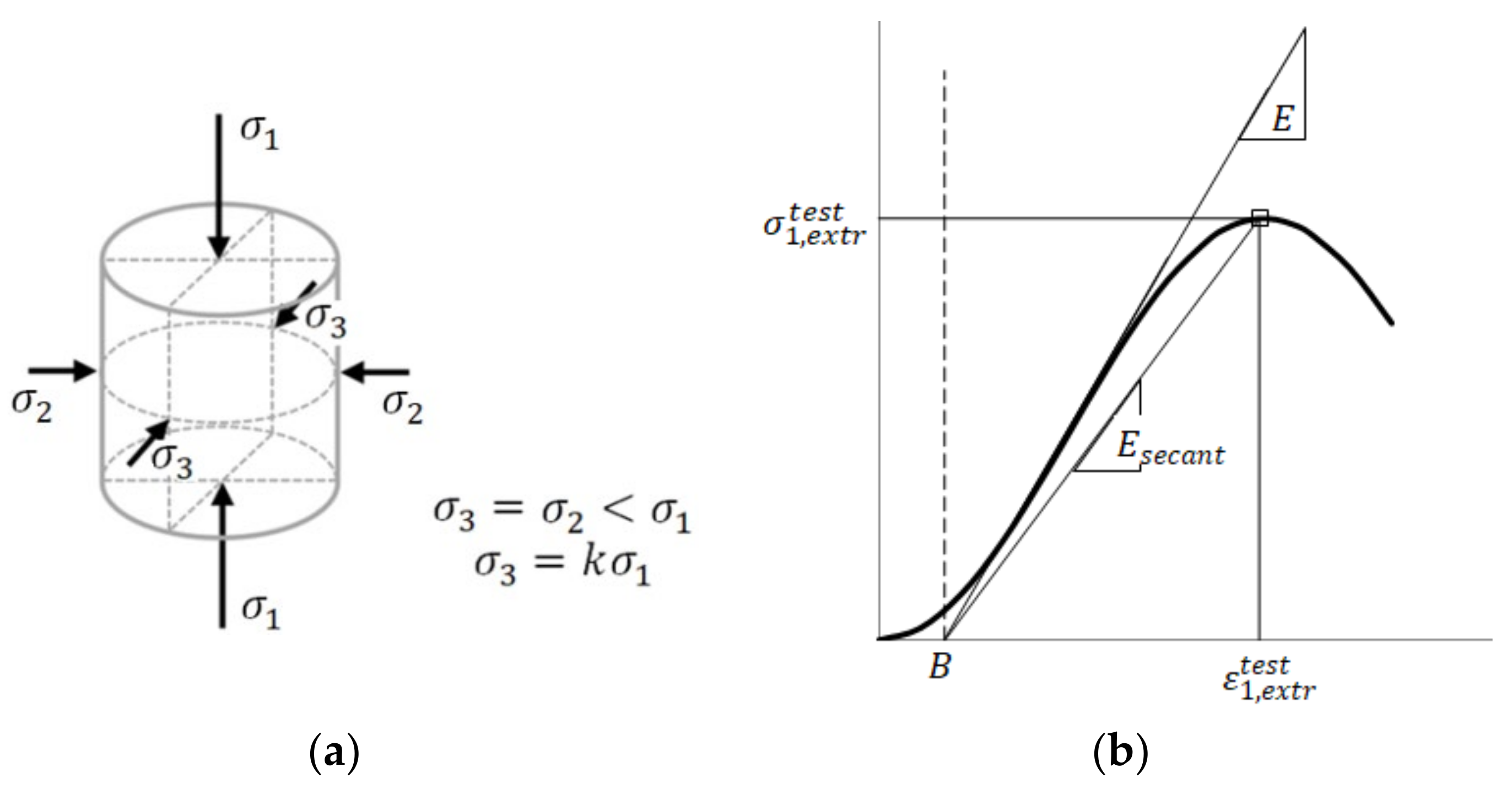
• The full load–displacement compression curve with axisymmetric lateral proportional pressure in accordance with Figure 1a is analytically described by one Equation (28);
• The linear dependence for determining the effective stress of a brittle material is substantiated (31);
• The ratio of the effective and secant elastic modulus is established (18);
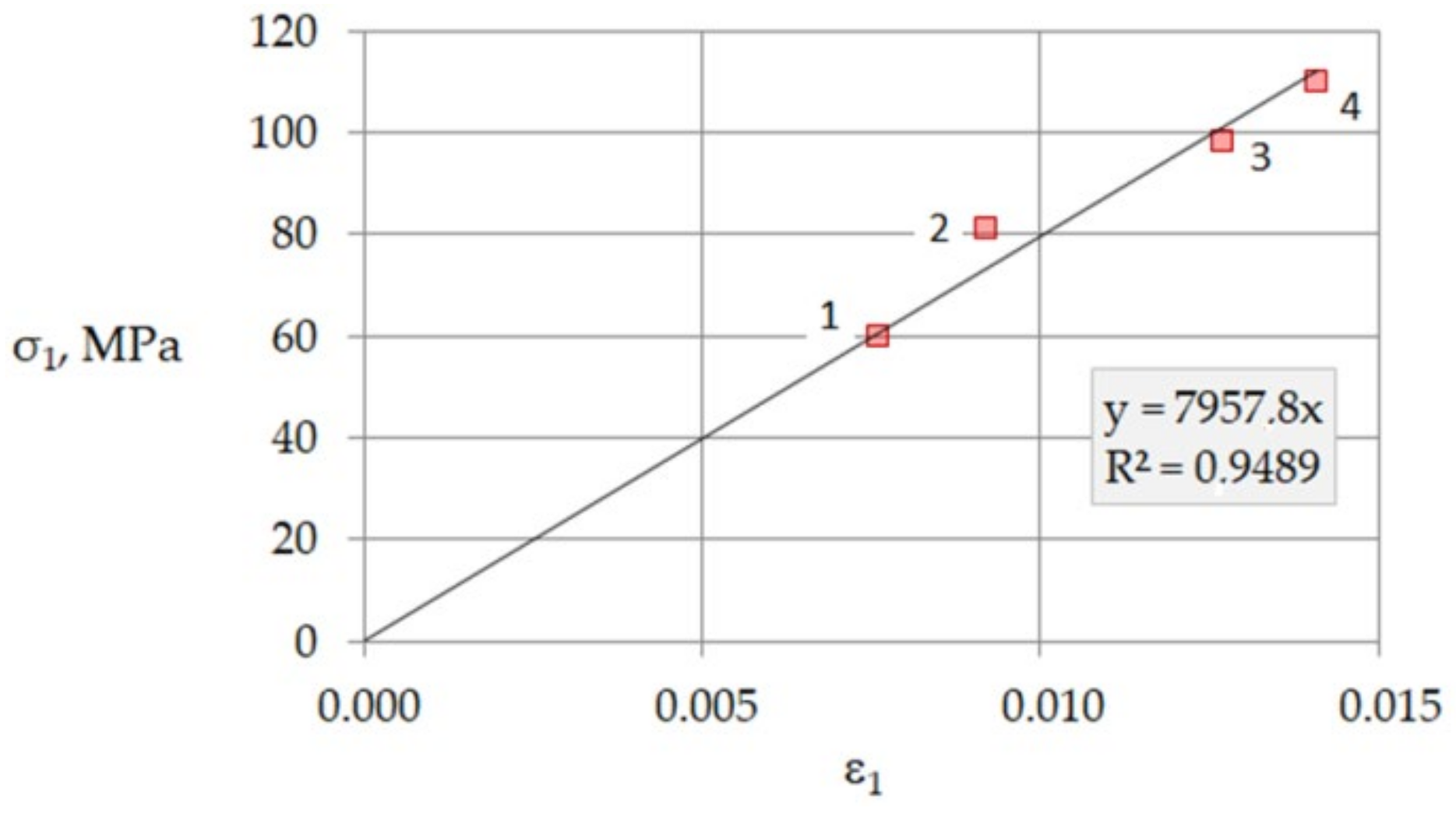
• Using the example of sandstone, it is proved that when compressing with proportional axisymmetric lateral pressure, the effective stress ${\tilde{\sigma }}_1$ (32) is the ratio of two nonlinear functions (28) and (30), which leads to a linear dependence of the effective stress on the strain ${\epsilon }_1$ (32) for the values of the Poisson’s ratio and the ratio of axial compressive and lateral pressures corresponding to the physical meaning of the problem;
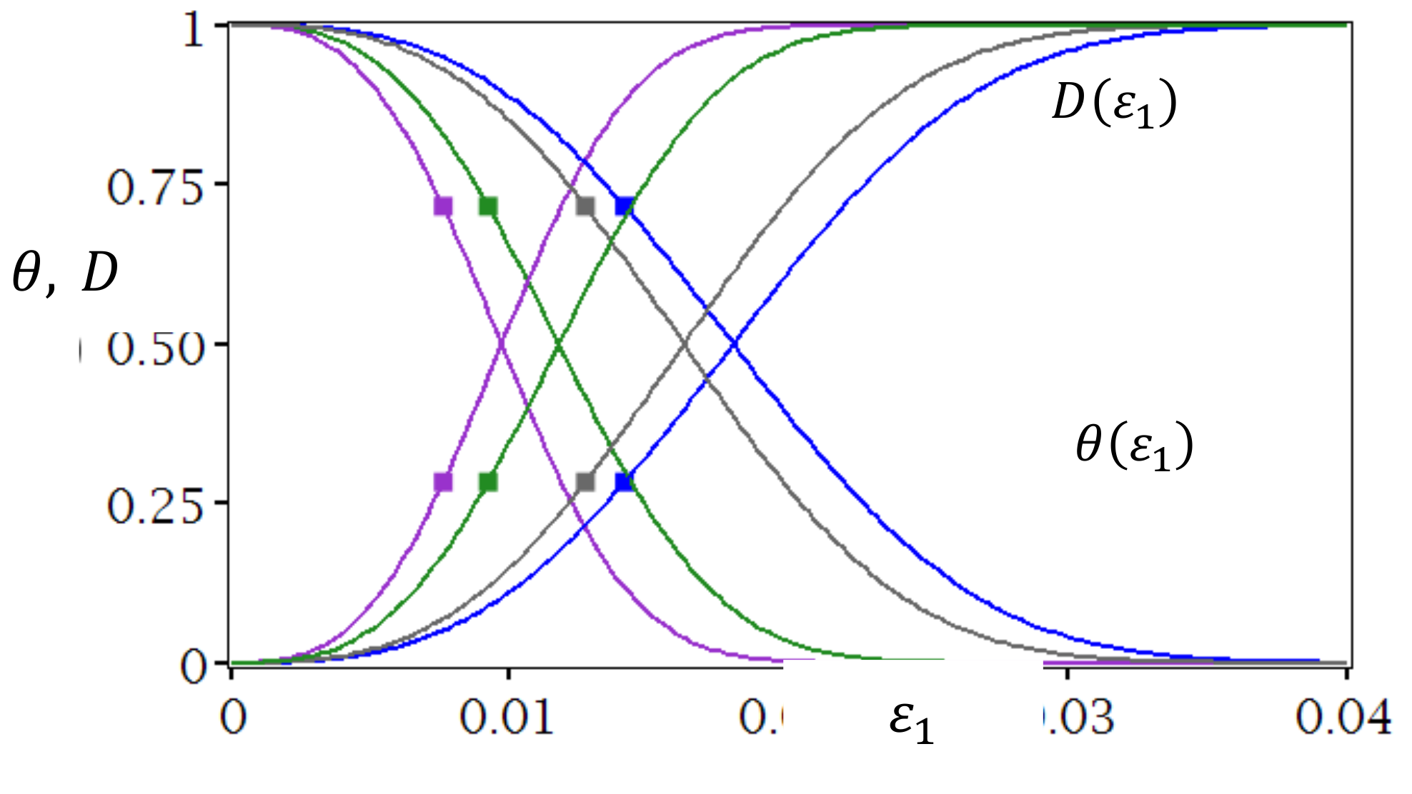
• The residual resource function for axial compression with lateral axially symmetric proportional pressure (30) is justified.
• With the use of the residual resource function, the damage function is proposed (31);
• The developed model implemented in the form of an algorithm (Section 3.1) is sufficiently adequate; however, this model does not take into account residual stresses appearing at the final stage of testing brittle materials for compression with lateral pressure. The appearance of residual stresses was recorded, for example, in the experiments of P. Y. Hou et al. [7]. Analysis of the conditions for the appearance of residual stresses using mathematical modeling may be a promising direction for the development of the topic.

3.3. Secant Modulus of Elasticity as a Physical Characteristic of the Material

In the comments to relations (18) and (19), it was assumed that the secant modulus of elasticity, defined as $E_{secant}={\sigma }_{1, extr}^{test}/{\epsilon }_{1, extr}^{test}$, can be considered as a physical characteristic of the material. A necessary condition for the adequacy of this assumption may be, as noted in the above comments, the localization of points with experimentally determined coordinates ${\epsilon }_{1, extr}^{test}$ and ${\sigma }_{1, extr}^{test}$ on a straight line whose equation ${\sigma }_1=E_{secant}{\epsilon }_1$, where $E_{secant}={\sigma }_{1, extr}^{test}/{\epsilon }_{1, extr}^{test}$. This straight line (Figure 4) is constructed using the experimental results mentioned above by P.Y. Hou et al. [7], which are shown in Table 2. The point numbers in Figure 4 coincide with the row numbers in Table 2.

Commenting on Figure 4, we note that points with experimentally determined coordinates ${\epsilon }_{1, extr}^{test}$ and ${\sigma }_{1, extr}^{test}$ are localized on a straight line whose equation is $E_{secant}=$ 12,140 MPa, where $E_{secant}={\sigma }_{1, extr}^{test}/{\epsilon }_{1, extr}^{test}=$ 12,193 MPa, which differs little from the average value of $E_{secant}=$ 12,140 MPa (Table 2). Consequently, in this case, the assumption formulated above about the secant modulus of elasticity is confirmed. Despite this, the issue remains debatable, since a small amount of sandstone sample was considered, and other rocks were not considered; therefore, verification should be considered conditional.

Nevertheless, the practical significance of the conditionally verified regularity lies in its possible use for predicting the behavior of brittle materials under axial compression with proportional lateral axisymmetric pressure. For example, the modulus of elasticity can be experimentally determined under uniaxial compression without limiting pressure (point 1 in Figure 4 and row 1 in Table 2). In addition, one of the three values ($E_{secant}$, ${\sigma }_{1, extr}^{test}$ and ${\epsilon }_{1, extr}^{test}$) can be determined if only two of them are known.

It should be borne in mind that the calculations discussed above (Section 3.1) should be performed with a sufficiently high accuracy.

Summing up the results presented above, it is legitimate to formulate the question: Will these results meet the requirements of other experiments known from the literature? The answer to this question will be received as part of the discussion of the above research results.

4. Results and Discussion

To create a more solid basis for discussion, we will consider another example of applying the algorithm presented in Section 3.1 to modeling the state of red sandstone.

4.1. Example 2: Red Sandstone

By analogy with Example 1 (Section 3.2), we will discuss the application of the proposed algorithm (Section 3.1) to modeling the mechanical state of red sandstone, using as initial data the test results from the work of W. Zhang et al. [13] (

Table 3. Иcxoдныe дaнныe и нeкoтoрыe рeзультaты вычиcлeний для крacнoгo пecчaникa.

Sample Number	Poisson’s Ratio ν	${\mathit{\sigma }}_{\mathit{c}\mathit{o}\mathit{n}\mathit{f}}$ (MPa)	Axial Stress Peak $({\mathit{\sigma }}_{1,\mathit{e}\mathit{x}\mathit{t}\mathit{r}}^{\mathit{t}\mathit{e}\mathit{s}\mathit{t}})$ (MPa)	$\mathit{k}$ $\left(\frac{{\mathit{\sigma }}_{\mathit{c}\mathit{o}\mathit{n}\mathit{f}}}{{\mathit{\sigma }}_{1,\mathit{e}\mathit{x}\mathit{t}\mathit{r}}^{\mathit{t}\mathit{e}\mathit{s}\mathit{t}}}\right)$	${\mathit{\mu }}^{\left(\mathit{k}\right)}$	Axial Strain at the Peak $({\mathit{\epsilon }}_{1,\mathit{e}\mathit{x}\mathit{t}\mathit{r}}^{\mathit{t}\mathit{e}\mathit{s}\mathit{t}})$	${\mathit{E}}_{\mathit{s}\mathit{e}\mathit{c}\mathit{a}\mathit{n}\mathit{t}}$ $\left(\frac{{\mathit{\sigma }}_{1,\mathit{e}\mathit{x}\mathit{t}\mathit{r}}^{\mathit{t}\mathit{e}\mathit{s}\mathit{t}}}{{\mathit{\epsilon }}_{1,\mathit{e}\mathit{x}\mathit{t}\mathit{r}}^{\mathit{t}\mathit{e}\mathit{s}\mathit{t}}}\right)$ (MPa)	$\tilde{\mathit{E}}$ (MPa)
1	0.189	5	59.70	0.0838	1.0111	0.0076	7855	10,966
2	0.165	10	80.99	0.1235	1.0259	0.0092	8794	12,276
3	0.188	15	98.21	0.1527	1.0389	0.0127	7733	10,795
4	0.189	20	110.12	0.1816	1.0562	0.0141	7810	10,903

).

The results of the calculations using the algorithm from Section 3.1 for samples 1,…, 4, the characteristics of which are given in Table 3, are presented graphically in Figure 5.

Commenting on Figure 2, Figure 3, Figure 4, Figure 5, Figure 6 and Figure 7, we note that the patterns of behavior of the two varieties of sandstone are similar. The noticeable deviation of point 2 from the straight line in Figure 7 is explained by the heterogeneity of the samples due to the influence of random factors on the modulus of elasticity and other physical characteristics of the sample material. On the other hand, the differences between the two varieties of sandstone, reflected in Figure 2, Figure 4, Figure 5 and Figure 7, as well as some anomaly of curve 2 (Figure 5) and point 2 (Figure 7), are quantitatively identified using the secant modulus of elasticity, defined as $E_{secant}={\sigma }_{1,extr}^{test}/{\epsilon }_{1,extr}^{test}$, which indicates the expediency of using the secant modulus of elasticity, defined in the form of such a ratio as one of the characteristics of the physical properties of a brittle material.

4.2. Comments

The results presented above do not contradict the studies of other authors [31,32,33,34,35]. Our study of axial compression with proportional lateral pressure (Figure 1a) is based on the assumption that the modulus of elasticity, as a physical characteristic of a brittle material, does not change during the force action. The same assumption was used in [17,23], but only for axial compression without lateral pressure. The results of tests of cylindrical samples made of cement-stabilized soil of low strength (1.23 MPa), known from the literature, can serve as confirmation of the adequacy of this assumption [30]. The cited work shows a stress–strain graph during loading and unloading in the pre-peak and post-peak states of a sample of the specified brittle material. This graph shows straight lines, the angle of inclination of which is the same in both the pre-peak and post-peak states of the sample; this means that the modulus of elasticity of this material is the same before and after the peak, because the angle of inclination of these straight lines determines the magnitude of the elastic modulus of the material (Figure 5 in the article [31]).

Comparing the theoretical and experimental data, we must take into account some uncertainties, namely, the unavoidable so-called imperfection of the sample material [32,33] and the influence of equipment characteristics on test results [7,8], as well as simplifications in the modeling methodology discussed above. Taking into account these realities, it is possible to find confirmations of approximate values of the elastic modulus before and after the stress peak in other published graphs of experimental stress–strain dependences for axial compression of sandstone at lateral pressure (relevant examples can be found in papers [34,35]). Nevertheless, the results presented above do not exclude discussion, and therefore it is necessary to continue the search on the affected topic, taking into account theoretical and applied aspects [36,37,38].

5. Conclusions

In this paper, an analytical model and algorithm were developed to study the mechanical state of a brittle material on the example of sandstone under axial compression and axisymmetric proportional lateral pressure. During the development of the model, methods of modeling mechanical systems based on new ideas of fracture mechanics were used.

As for the innovative aspects of this work, we note the following. In this paper, an analytical model of the dependence of the load on displacement during compression of a brittle material with proportional axisymmetric lateral pressure is substantiated. For the same loading conditions, analytical relations were obtained to predict the value of the residual life of the load-bearing capacity and the damage function of the brittle material. Furthermore, the relations for analytical determination of effective stresses and effective modulus of elasticity were found.

For practical application of the research results, a calculation algorithm is proposed, and examples of its application were considered. The simulation results are consistent with the experimental data known from the literature. It is proved that as the deformations of the brittle material sample increase, the effective stress increases to the final point of degradation and destruction of the sample. At the same time, the apparent stresses increase, reach a peak, and then decrease to the final point on the descending load–displacement branch. Thus, modeling the dependence of effective stresses on deformations during compression of brittle material in combination with lateral proportional axisymmetric pressure explains the destruction of such materials on the descending branch of the load–displacement diagram.

This study is a continuation of the earlier considered simpler case of uniaxial compression of brittle material without taking into account lateral pressure. Taking into account lateral pressure is important for practice; however, the issues of modeling residual stresses during compression with lateral pressure remain outside the scope of this article, which limits the scope of practical application of the developed model. Nevertheless, the authors suggest that, in this paper, another step has been taken towards a better understanding of the complex problem of the mechanical behavior and destruction of brittle materials during their compression in combination with lateral pressure. This implies that the work has the prospect of continuation.

References

1. Mohammadnejad, M.; Liu, H.; Chan, A.; Dehkhoda, S.; Fukuda, D. An overview on advances in computational fracture mechanics of rock. Geosystem Eng. 2021, 24, 206–229. [Google Scholar] [CrossRef]
2. Iskander, M.; Shrive, N. Fracture of brittle and quasi-brittle materials in compression: A review of the current state of knowledge and a different approach. Theor. Appl. Fract. Mech. 2018, 97, 250–257. [Google Scholar] [CrossRef]
3. Oucif, C.; Mauludin, L.M. Continuum Damage-Healing and Super Healing Mechanics in Brittle Materials: A State-of-the-Art Review. Appl. Sci. 2018, 8, 2350. [Google Scholar] [CrossRef] [Green Version]
4. Ju, M.; Li, X.; Li, X.; Zhang, G. A review of the effects of weak interfaces on crack propagation in rock: From phenomenon to mechanism. Eng. Fract. Mech. 2022, 263, 108297. [Google Scholar] [CrossRef]
5. Huang, Y.H.; Yang, S.Q.; Tian, W.L.; Wu, S.Y. Experimental and DEM study on failure behavior and stress distribution of flawed sandstone specimens under uniaxial compression. Theor. Appl. Fract. Mech. 2022, 118, 103266. [Google Scholar] [CrossRef]
6. Cai, M.; Hou, P.Y.; Zhang, X.W.; Feng, X.T. Post-peak stress–strain curves of brittle hard rocks under axial-strain-controlled loading. Int. J. Rock Mech. Min. Sci. 2021, 147, 104921. [Google Scholar] [CrossRef]
7. Hou, P.Y.; Cai, M.; Zhang, X.W.; Feng, X.T. Post-peak Stress–Strain Curves of Brittle Rocks Under Axial and Lateral-Strain-Controlled Loadings. Rock Mech. Rock Eng. 2021, 147, 855–884. [Google Scholar] [CrossRef]
8. Chen, X.; Yu, J.; Tang, C.; Li, H.; Wang, S. Experimental and Numerical Investigation of Permeability Evolution with Damage of Sandstone Under Triaxial Compression. Rock Mech. Rock Eng. 2017, 50, 1529–1549. [Google Scholar] [CrossRef]
9. Zhang, Y.; Wang, L.; Zi, G.; Zhang, Y. Mechanical Behavior of Coupled Elastoplastic Damage of Clastic Sandstone of Different Burial Depths. Energies 2020, 13, 1640. [Google Scholar] [CrossRef] [Green Version]
10. Li, H.; Wang, J.; Li, H.; Wei, S.; Li, X. Experimental Study on Deformation and Strength Characteristics of Interbedded Sandstone with Different Interlayer Thickness under Uniaxial and Triaxial Compression. Processes 2022, 10, 285. [Google Scholar] [CrossRef]
11. Shahin, A.; Myers, M.T.; Hathon, L.A. Borehole Geophysical Joint Inversion to Fully Evaluate Shaly Sandstone Formations. Appl. Sci. 2022, 12, 1255. [Google Scholar] [CrossRef]
12. Xu, T.; Fu, M.; Yang, S.Q.; Heap, M.J.; Zhou, G.L. A numerical meso-scale elasto-plastic damage model for modeling the deformation and fracturing of sandstone under cyclic loading. Rock Mech. Rock Eng. 2021, 54, 4569–4591. [Google Scholar] [CrossRef]
13. Zhang, W.; Chen, Y.Y.; Guo, J.P.; Wu, S.S.; Yan, C.Y. Investigation into Macro-and Microcrack Propagation Mechanism of Red Sandstone under Different Confining Pressures Using 3D Numerical Simulation and CT Verification. Geofluids 2021, 2021, 2871687. [Google Scholar] [CrossRef]
14. Mudunuru, M.K.; Panda, N.; Karra, S.; Srinivasan, G.; Chau, V.T.; Rougier, E.; Hunter, A.; Viswanathan, H.S. Surrogate Models for Estimating Failure in Brittle and Quasi-Brittle Materials. Appl. Sci. 2019, 9, 2706. [Google Scholar] [CrossRef] [Green Version]
15. Wang, L.; Su, H.; Chen, S.; Qin, Y. Nonlinear dynamic constitutive model of frozen sandstone based on Weibull distribution. Adv. Civ. Eng. 2020, 2020, 6439207. [Google Scholar] [CrossRef]
16. Yang, B.; Qin, S.; Xue, L.; Chen, H. The reasonable range limit of the shape parameter in the Weibull distribution for describing the brittle failure behavior of rocks. Rock Mech. Rock Eng. 2021, 54, 3359–3367. [Google Scholar] [CrossRef]
17. Kolesnikov, G. Damage Function of a Quasi-Brittle Material, Damage Rate, Acceleration and Jerk during Uniaxial Compression: Model and Application to Analysis of Trabecular Bone Tissue Destruction. Symmetry 2021, 13, 1759. [Google Scholar] [CrossRef]
18. Åström, J.A. Statistical models of brittle fragmentation. Adv. Phys. 2006, 55, 247–278. [Google Scholar] [CrossRef]
19. Shah, K.S.; Mohd Hashim, M.H.; Rehman, H.; Ariffin, K.S. Application of Stochastic Simulation in Assessing Effect of Particle Morphology on Fracture Characteristics of Sandstone. J. Min. Environ. 2021, 12, 969–986. [Google Scholar]
20. Wu, T.; Liu, Y.; Liu, X.; Zhang, B. Meso-scale stochastic modeling for mechanical properties of structural lightweight aggregate concrete. Mater. Struct. 2022, 55, 17. [Google Scholar] [CrossRef]
21. Hu, B.; Zhang, Z.; Li, J.; Xiao, H.; Wang, Z. Statistical Damage Model of Rock Structural Plane Considering Void Compaction and Failure Modes. Symmetry 2022, 14, 434. [Google Scholar] [CrossRef]
22. Drugan, W.J. Dynamic fragmentation of brittle materials: Analytical mechanics-based models. J. Mech. Phys. Solids 2001, 49, 1181–1208. [Google Scholar] [CrossRef]
23. Kolesnikov, G.; Meltser, R. A Damage Model to Trabecular Bone and Similar Materials: Residual Resource, Effective Elasticity Modulus, and Effective Stress under Uniaxial Compression. Symmetry 2021, 13, 1051. [Google Scholar] [CrossRef]
24. Baldwin, R.; North, M.A. Stress-Strain Curves of Concrete at High Temperature—A review. Fire Research Note, 1969, No. 785. 3-14. Available online: http://www.iafss.org/publications/frn/785/-1/view/frn_785.pdf (accessed on 18 October 2021).
25. Li, Y.; Chen, Y.F.; Zhou, C.B. Effective stress principle for partially saturated rock fractures. Rock Mech. Rock Eng. 2016, 49, 1091–1096. [Google Scholar] [CrossRef]
26. Stojković, N.; Perić, D.; Stojić, D.; Marković, N. New stress-strain model for concrete at high temperatures. Teh. Vjesn. 2017, 24, 863–868. [Google Scholar]
27. Stepanova, L.V.; Igonin, S.A. Rabotnov damage parameter and description of delayed fracture: Results, current status, application to fracture mechanics, and prospects. J. Appl. Mech. Tech. Phys. 2015, 56, 282–292. [Google Scholar] [CrossRef]
28. Wen, T.; Tang, H.; Ma, J.; Liu, Y. Energy Analysis of the Deformation and Failure Process of Sandstone and Damage Constitutive Model. KSCE J. Civ. Eng. 2019, 23, 513–524. [Google Scholar] [CrossRef]
29. Zhao, B.; Li, Y.; Huang, W.; Yang, J.; Sun, J.; Li, W.; Zhang, L. Mechanical characteristics of red sandstone under cyclic wetting and drying. Environ. Earth Sci. 2021, 80, 738. [Google Scholar] [CrossRef]
30. Kolesnikov, G. Analysis of Concrete Failure on the Descending Branch of the Load-Displacement Curve. Crystals 2020, 10, 921. [Google Scholar] [CrossRef]
31. Vogler, U.; Stacey, T. The influence of test specimen geometry on the laboratory-determined Class II characteristics of rocks. J. S. Afr. Inst. Min. Metall. 2016, 116, 987–1000. [Google Scholar] [CrossRef] [Green Version]
32. Huang, Z.; Gu, Q.; Wu, Y.; Wu, Y.; Li, S.; Zhao, K.; Zhang, R. Effects of confining pressure on acoustic emission and failure characteristics of sandstone. Int. J. Min. Sci. Technol. 2021, 31, 963–974. [Google Scholar] [CrossRef]
33. Wang, Z.; Thomas, B.; Zhang, W.; Gu, D. A novel random angular bend (RAB) algorithm and DEM modeling of thermal cracking responses of sandstone. Geomech. Energy Environ. 2022, 100335. [Google Scholar] [CrossRef]
34. Cheng, C.; Li, X.; Li, S.; Zheng, B. Failure Behavior of Granite Affected by Confinement and Water Pressure and Its Influence on the Seepage Behavior by Laboratory Experiments. Materials 2017, 10, 798. [Google Scholar] [CrossRef] [PubMed] [Green Version]
35. Jia, C.; Zhang, Q.; Wang, S. Experimental Investigation and Micromechanical Modeling of Elastoplastic Damage Behavior of Sandstone. Materials 2020, 13, 3414. [Google Scholar] [CrossRef]
36. Lin, Q.; Cao, P.; Wen, G.; Meng, J.; Cao, R.; Zhao, Z. Crack coalescence in rock-like specimens with two dissimilar layers and pre-existing double parallel joints under uniaxial compression. Int. J. Rock Mech. Min. Sci. 2021, 139, 104621. [Google Scholar] [CrossRef]
37. Lin, Q.; Cao, P.; Meng, J.; Cao, R.; Zhao, Z. Strength and failure characteristics of jointed rock mass with double circular holes under uniaxial compression: Insights from discrete element method modelling. Theor. Appl. Fract. Mech. 2020, 109, 102692. [Google Scholar] [CrossRef]
38. Lin, Q.; Cao, P.; Cao, R.; Lin, H.; Meng, J. Mechanical behavior around double circular openings in a jointed rock mass under uniaxial compression. Arch. Civ. Mech. Eng. 2020, 20, 19. [Google Scholar] [CrossRef] [Green Version]
Figure 1. (a) Axial compression and proportional axisymmetric confining pressure. For stresses ( σ 1 ,   σ 2 ,   σ 3 ), the same sign rule is used as in [28]. (b) A typical load–strain plot (by analogy with [29]). The origin of the coordinates is shifted to point B .
Symmetry 14 00796 g001
Figure 2. (a) Dependences of the apparent and effective stresses on strain ε 1 , respectively, shown by solid curves and dashed straight lines. The line numbers correspond to the row numbers in Table 2. The peak stress values σ 1 are located almost on the same straight line, the angle of inclination of which is determined by the secant modulus of elasticity E s e c a n t . The asterisks mark the points at which, according to the experiments [7], accelerated destruction begins in the post-peak state of the sample. (b) enlarged fragment of the plot.
Symmetry 14 00796 g002
Figure 3. The functions plots of residual resource θ ε 1 and damage D ε 1 = 1 θ ε 1 for samples 1,…, 5 in Figure 2. Markers (colored squares) mark the values of functions θ and D if ε 1 = ε 1 ,   e x t r t e s t ; in this case θ = e 1 / 3 0.72 and D = 0.28 . The asterisks mark the points at which, according to the experiments [7], accelerated fracture begins in the post-peak state of the material.
Symmetry 14 00796 g003
Figure 4. Stresses peak values (according to Fig. 2) are on a straight line, the equation of which has the form σ 1 = E s e c a n t ε 1 , E s e c a n t = 12 , 193   MPa .
Symmetry 14 00796 g004
Figure 5. (a) The dependences of the apparent σ 1 and effective ( σ ˜ 1 ) stresses on the strain of ε 1 , respectively, are shown with solid curves and dotted straight lines. The line numbers correspond to the row numbers in Table 2. The peak stress values σ 1 for samples 1, 3 and 4 are localized on almost the same straight line, the angle of inclination of which is determined by the secant elastic modulus E s e c a n t (b) enlarged fragment of the plot.
Symmetry 14 00796 g005
Figure 6. Plots of residual resource functions θ ε 1 and damage D ε 1 for the initial data from Table 3. Markers (squares) mark the values of functions θ and D if ε 1 = ε 1 ,   e x t r t e s t , which corresponds to the peak values σ 1 = σ 1 , e x t r t e s t (Figure 1b); in this case = e 1 / 3 0.72 and D = 0.28 .
Symmetry 14 00796 g006
Figure 7. The peak stress values shown above in Figure 5 are on a straight line, the equation of which σ 1 = E s e c a n t ε 1 , E s e c a n t 7957   MPa .
Symmetry 14 00796 g007