Numerical Solution of the Linear Fractional Delay Differential Equation Using Gauss–Hermite Quadrature

Abstract

Fractional order differential equations often possess inherent symmetries that play a crucial role in governing their dynamics in a variety of scientific fields. In this work, we consider numerical solutions for fractional-order linear delay differential equations. The numerical solution is obtained via the Laplace transform technique. The quadrature approximation of the Bromwich integral provides the foundation for several commonly employed strategies for inverting the Laplace transform. The key factor for quadrature approximation is the contour deformation, and numerous contours have been proposed. However, the highly convergent trapezoidal rule has always been the most common quadrature rule. In this work, the Gauss–Hermite quadrature rule is used as a substitute for the trapezoidal rule. Plotting figures of absolute error and comparing results to other methods from the literature illustrate how effectively the suggested approach works. Functional analysis was used to examine the existence of the solution and the Ulam–Hyers (UH) stability of the considered equation.

1. Introduction

Fractional calculus (FC) is a branch of mathematics which generalizes the classical calculus. A close connection between FC and the dynamics of complex real-world problems exists. Despite a long history, the concept of FC has not been applied in engineering or other science fields. However, in the last two decades the FC has attracted a remarkable amount of attention from the research community. It has been pointed out that fractional order operators are very helpful in describing various real world phenomena [1], for example rheology, signal analysis, viscoelasticity, continuum mechanics, polymeric chemistry, etc [2,3]. Differential equations involving fractional order operators arising in engineering and other sciences describe nature adequately in terms of symmetry properties [4]. The authors of [5] studied hyperchaotic behavior of fractional order problems including fractional operator with two fractional orders. Tang et al. [6] modeled the dynamical behaviors of different stages of breast cancer and used the Adams–Bashforth technique for the numerical simulations. The authors of [7] analyzed the dynamics of the dengue infection by formulating a compartmental model of fractional order. In [8], the authors modeled tumor-immune cells interactions using operators from fractional calculus.

The delay or lags are encountered very often in many real-world problems, for example, immunology [9], population dynamics and epidemiology [10], drug therapy [11], respiratory systems [12], etc. Time-fractional delay differential equations (FDDEs) usually do not have analytical solutions and can be solved only by using some numerical techniques. The development of efficient numerical methods for solving FDDEs has received great attention recently. For instance, Morgado et al. [13] discussed the existence and uniqueness of the solution to FDDEs. They utilized the fractional backward difference method to study the solution to the considered FDDEs. The authors of [14] used the finite difference method for obtaining the approximate solution of FDDEs. In [15], the authors developed a novel method for solving FDDEs and compared their results with the fractional Adams method and fractional predictor–corrector method. The authors of [16] solved FDDEs including Riemann–Liouville and Liouville–Caputo fractional operators using the shifted Jacobi polynomials. Chishti et al. [17] utilized the extended versions of the two numerical methods, the fractional finite difference method and the predictor–corrector method for the approximation of FDDEs. In [18], the authors solved a class of FDDEs including Liouville–Caputo fractional operator using the orthogonal Chelyshkov functions. Naseem et al. [19] used the differential transform method for the analytical approximation of FDDE. Rebenda and Šmarda [20] used a differential transformation approach for solving functional differential equations with multiple delays. Li et al. [21] utilized a spectral scheme to investigate the numerical solution of fractional stochastic delay differential equations with a comprehensive stability analysis. The authors of [22] established a comprehensive analysis of a general class of FDDEs with the Caputo–Fabrizio fractional derivative. Sher et al. [23] used prior estimate method to investigate the existence and uniqueness of solution for a class of evolution fractional order differential equations with a proportional delay using the Caputo derivative. They also studied different kinds of Ulam stability. The authors of [24] studied the asymptotic stability of nonlinear fractional-order differential equations with multiple delays under the Caputo’s fractional derivative with $1<\alpha <2.$

The Laplace transform is a powerful method for solving differential equations. However, for computational work, this technique has not become popular, as researchers have focused on discretizaion methods such as finite difference, finite element, and boundary elements, possibly coupled with Runge–Kutta or linear multistep methods for integration in time. This lack of interest from the research community is possibly due to two factors: (i) the Laplace transform cannot handle nonlinear differential equations; (ii) the numerical inversion of the Laplace transform is very hard to compute. Despite these drawbacks, Laplace transform methods have been utilized recently by researchers, particularly in the area of linear PDEs [25,26,27,28,29]. The solution of many differential equations may be found in terms of the Laplace transform which is then, however, very difficult for inversion via the techniques of complex analysis. Many strategies have been suggested for inverting the Laplace transform. However, the Laplace transform cannot be directly applied to DDEs. In [30], the authors have recently proposed an effective Laplace transform technique to solve second-order DDEs. The author derives some reliable theoretical results to transform the given DDE to an equivalent algebraic equation in the Laplace transform space and solves the transformed equation for the unknown. Finally, the exact solution of the considered DDE is obtained using the techniques of complex analysis. However, sometimes, using the Laplace transform for many DDEs, the analytical inversion of the Laplace transform becomes very laborious and difficult. Thus, the best alternative is to utilize some numerical techniques. The main advantages of the Laplace transform are as follows:

• The Laplace transform converts the complex FDDE into a simpler algebraic equation in the Laplace domain. This transformation significantly reduces the challenge of solving differential equations with fractional derivatives and delays, which leads to a more regulated and efficient procedure.
• The Laplace transform effectively incorporates the initial conditions into the transformed equation. This feature is particularly beneficial for FDDEs because it makes it possible to provide initial states easily without the need for more intricate manipulations.
• The Laplace transform method is applicable to a large class of FDDEs with different kinds of fractional derivative and delay terms. This adaptability makes it a powerful tool in a variety of fields such as applied mathematics, physics, engineering, and control theory.

In this work, our objective was to use the method developed in [30] for solving FDDEs. We employ the Gauss–Hermite quadrature method for numerical inversion of the Laplace transform. We consider a fractional order DDE given as follows:

$$D_x^{\beta }y\left(x\right)=f\left(x\right)+A_{1}y\left(x\right)+A_{2}y(x-\chi ),\beta \in (0,1],x>0,$$

(1)

$$y\left(x\right)=\varrho \left(x\right),-\chi \le x\le 0,y\left(0\right)={\gamma }_1,$$

(2)

where $f:[0,T]\to \mathbb{R}$ is the linear continuous function, $A_1,A_2,{\gamma }_1$ are real constants, $\varrho \left(x\right)$ is the known sufficiently smooth real valued function, and $\chi \in {\mathbb{R}}^{+}$ is a finite delay.

2. Preliminaries

Let $\mathcal{J}=[0,T],$ and $\Theta =C(\mathcal{J},R),$; then, for any function $y\in \Theta$, the supremum norm $\parallel .\parallel$ on $\Theta$ is defined as

$$\parallel y\parallel =\underset{x\in \mathcal{J}}{sup}\left|y\left(x\right)\right|.$$

Definition 1

([3]). Let $\beta >0$ and let $f\left(x\right)$ be piecewise continuous on $(0,\infty )$ and integrable on any finite subinterval of $[0,\infty ).$ Then, for $x>0$, we call

$$I_{0+}^{\beta }f\left(x\right)=\frac{1}{\Gamma \left(\beta \right)}{\int }_0^x{(x-s)}^{\beta -1}f\left(s\right)ds,$$

the Riemann–Liouville fractional integral of $f\left(x\right)$ of order $\beta .$

Definition 2

([3]). If $f\in C^p[0,T],p\in \mathbb{N},$ and $\beta \in (p-1,p],$ then the Caputo fractional derivative of order β is defined as

$$D_x^{\beta }f\left(x\right)=\frac{1}{\Gamma (p-\beta )}{\int }_0^x\frac{\frac{d^{p}f\left(s\right)}{d{s}^p}}{{(x-s)}^{\beta -p+1}}ds, x>0,$$

(3)

where $p=\left[\beta \right]+1$ with $\left[\beta \right]$ the integer part of $\beta .$ The above derivative exists if the integral on the right side converges; further, if $0<\beta \le 1,$ then Equation (3) can be written as follows:

$$D_x^{\beta }f\left(x\right)=\frac{1}{\Gamma (1-\beta )}{\int }_0^x\frac{\frac{df\left(s\right)}{ds}}{{(x-s)}^{\beta }}ds,$$

provided the integral on the right side converges.

Lemma 1

([31]). Let $0<\beta \le 1$ with f continuous on $\mathcal{J}\times J$, where $J\subset \mathbb{R}$ is an unbounded interval. If $y\left(x\right)$ is continuous on $(0,T]$ and $y,x\to f(x,y(x\left)\right)$ belongs to $L^1[0,T],$ then $y\left(x\right)$ satisfies the initial value problem

$$D_x^{\beta }y\left(x\right)=f(x,y\left(x\right)),x\in \mathcal{J},$$

$$y\left(0\right)=y_0,$$

if and only if it satisfies the following Volterra integral equation:

$$y\left(x\right)=y_0+\frac{1}{\Gamma \left(\beta \right)}{\int }_0^x{(x-s)}^{\beta -1}f(s,y\left(s\right))ds.$$

Definition 3

([3]). Let $y\left(x\right)$ be a piecewise continuous real valued function defined for $x>0$; then, its Laplace transform (LT) is denoted and defined as follows:

$$\widehat{y}\left(\mu \right)=\mathcal{L}\left\{y\left(x\right)\right\}={\int }_0^{\infty }{e}^{-\mu x}y\left(x\right)dx.$$

(4)

Theorem 1

([3]). The LT of $D_x^{\beta }y\left(x\right)$ is defined as follows:

$$\mathcal{L}\left\{D_x^{\beta }y\left(x\right)\right\}={\mu }^{\beta }\mathcal{L}\left\{y\left(x\right)\right\}-\sum _{k=0}^{p-1}{\mu }^{\beta -k-1}{y}^k\left(0\right),p-1<\beta <p,p\in \mathbb{N}.$$

(5)

Theorem 2

([30]). Let $\varrho \left(x\right)$, ${\varrho }^{\prime }\left(x\right)$ be continuous on the interval $[-\chi ,0]$; then, the LT of $y(x-\chi )$ is given as follows:

$$\mathcal{L}\left\{y(x-\chi )\right\}=\overline{\varrho }\left(\mu \right)+exp(-\mu \chi )\mathcal{L}\left\{y\left(x\right)\right\},$$

Also, the LT of $y^{\prime }(x-\chi )$ is given as follows:

$$\mathcal{L}\left\{y^{\prime }(x-\chi )\right\}=\overline{\overline{\varrho }}\left(\mu \right)+exp(-\mu \chi )\mathcal{L}\left\{y^{\prime }\left(x\right)\right\},$$

where

$$\overline{\varrho }\left(\mu \right)={\int }_{-\chi }^0{e}^{-\mu (x+\chi )}\varrho \left(x\right)dx,$$

and

$$\overline{\overline{\varrho }}\left(\mu \right)={\int }_{-\chi }^0{e}^{-\mu (x+\chi )}{\varrho }^{\prime }\left(x\right)dx.$$

3. Existence

In this section, we study the existence of solution to Problems (1) and (2).

Lemma 2.

Let $0<\beta \le 1$ with f continuous on $\mathcal{J}\times J$, where $J\subset \mathbb{R}$ is an unbounded interval; then, the solution of the problem

$$D_x^{\beta }y\left(x\right)=f\left(x\right)+A_{1}y\left(x\right)+A_{2}y(x-\chi ),x\in \mathcal{J},$$

(6)

$$y\left(x\right)=\varrho \left(x\right),-\chi \le x\le 0,y\left(0\right)={\gamma }_1,$$

can be expressed as

$$y\left(x\right)={\gamma }_1+\frac{1}{\Gamma \left(\beta \right)}{\int }_0^x{(x-s)}^{\beta -1}[f\left(s\right)+A_{1}y\left(s\right)+A_{2}y(s-\chi )]ds,x\in \mathcal{J}.$$

Proof. 

Using Lemma (1), the solution of the initial value problem (6) can be written as

$$y\left(x\right)={\gamma }_1+\frac{1}{\Gamma \left(\beta \right)}{\int }_0^x{(x-s)}^{\beta -1}[f\left(s\right)+A_{1}y\left(s\right)+A_{2}y(s-\chi )]ds.$$

To prove the existence of solution to Problems (1) and (2), let us define an operator $\mathcal{S}:\Omega \to \Omega$ by

$$\mathcal{S}y\left(x\right)={\gamma }_1+\frac{1}{\Gamma \left(\beta \right)}{\int }_0^x{(x-s)}^{\beta -1}[f\left(s\right)+A_{1}y\left(s\right)+A_{2}y(s-\chi )]ds,x\in \mathcal{J}.$$

(7)

□

The following assumptions are needed for further analysis:

Hypothesis 1.

For a continuous function $\mathcal{L}\left(y\right),$ and a real constant $\mathcal{N}>0,$ the following Lipschitz conditions holds:

$$\begin{array}{cc} & |\mathcal{L}\left(y_1\right)-\mathcal{L}\left(y_2\right)|\le \mathcal{N}|y_1-y_2|.\hfill \end{array}$$

Hypothesis 2.

There exist ${\eta }_1>0,{\eta }_2>0$ such that

$$\begin{array}{cc} & |f(s,y_1,y_2)-f(s,{\widehat{y}}_1,{\widehat{y}}_2)|\le {\eta }_1|y_1-{\widehat{y}}_1|+{\eta }_2|y_2-{\widehat{y}}_2|.\hfill \end{array}$$

Theorem 3

(Schauder’s fixed point theorem [32]). Suppose that M is a nonempty, convex, compact subset of a Banach space Ω and that $\mathcal{S}:M\to M$ is a compact operator that maps M into itself. Then, $\mathcal{S}$ has a fixed point in M.

From the considered Problems (1) and (2), the equivalent integral form is obtained as

$$\begin{array}{c}\hfill y\left(x\right)=\left\{\begin{array}{c}{\gamma }_1+\frac{1}{\Gamma \left(\beta \right)}{\int }_0^x{(x-s)}^{\beta -1}f\left(s\right)ds+{\int }_0^x(x-s)[A_{1}y\left(s\right)+A_{2}y(s-\chi )]ds,x\in \mathcal{J},\hfill \\ \varrho \left(x\right),-\chi \le x\le 0.\hfill \end{array}\right.\end{array}$$

(8)

Since f is linear bounded function, we have $\left|f\left(x\right)\right|\le k_f,k_f>0$.

Theorem 4.

Under the hypothesis ${\mathbf{H}}_1$, the considered problem has a solution.

Proof. 

Let us define the Banach space $\Omega$ under the norm described by $\parallel y\parallel ={sup}_{x\in \mathcal{J}}\left|y\left(x\right)\right|.$ Consider a nonempty, convex, and compact subset M of $\Omega$ defined by $M=\{y:y\in B_r,\parallel y\left(x_1\right)-y\left(x_2\right)\parallel \le N\parallel x_1-x_2\parallel ,x_1,x_2\in \mathcal{J}\}.$

Define the operator $\mathcal{S}:M\to M$ by

$$\begin{array}{c}\hfill \mathcal{S}\left[y\left(x\right)\right]={\gamma }_1+\frac{1}{\Gamma \left(\beta \right)}{\int }_0^x{(x-s)}^{\beta -1}f\left(s\right)ds+\frac{1}{\Gamma \left(\beta \right)}{\int }_0^x{(x-s)}^{\beta -1}[A_{1}y\left(s\right)+A_{2}y(s-\chi )]ds,x\in \mathcal{J}.\end{array}$$

(9)

Let $y\in M$; then, to show that M is bounded, we use (9)

$$\begin{array}{ccc}\hfill \left|\mathcal{S}y\right(x\left)\right|& =& |{\gamma }_1+\frac{1}{\Gamma \left(\beta \right)}{\int }_0^x{(x-s)}^{\beta -1}f\left(s\right)ds+\frac{1}{\Gamma \left(\beta \right)}{\int }_0^x{(x-s)}^{\beta -1}[A_{1}y\left(s\right)+A_{2}y(s-\chi )]ds|\hfill \\ & \le & |{\gamma }_1|+\frac{1}{\Gamma \left(\beta \right)}{\int }_0^x{(x-s)}^{\beta -1}\left|f\left(s\right)\right|ds+\frac{1}{\Gamma \left(\beta \right)}{\int }_0^x{(x-s)}^{\beta -1}[A_1\left|y\left(s\right)\right|+A_2\left|y(s-\chi )\right|]ds\hfill \\ & \le & |{\gamma }_1|+\frac{k_f{T}^{\beta }}{\Gamma (\beta +1)}+\frac{N{A}_1}{\Gamma \left(\beta \right)}{\int }_0^x{(x-s)}^{\beta -1}+\frac{N{A}_2}{\Gamma \left(\beta \right)}{\int }_0^x{(x-s)}^{\beta -1}\hfill \\ & \le & |{\gamma }_1|+\frac{k_f{T}^{\beta }}{\Gamma (\beta +1)}+\frac{N{A}_1{T}^{\beta }}{\Gamma (\beta +1)}+\frac{N{A}_2{T}^{\beta }}{\Gamma (\beta +1)}\hfill \\ & =& \rho .\hfill \end{array}$$

which implies that

$$\parallel \mathcal{S}y\parallel \le \rho .$$

This shows that $\mathcal{S}$ is bounded. Obviously, we can claim that $\mathcal{S}$ maps bounded set to bounded sets into bounded sets.

To show that $\mathcal{S}$ is continuous, let $y_n$ in M since M is compact and contains all of its limit points. Therefore, $y_n\to y,\mathrm{as}n\to \infty$. Therefore, we take

$$\begin{array}{ccc}\hfill |\mathcal{S}{y}_n-\mathcal{S}y|& =& \frac{1}{\Gamma \left(\beta \right)}\left|{\int }_0^x{(x-s)}^{\beta -1}[A_1(y_n\left(s\right)-y\left(s\right))+A_2(y_n(s-\chi )-y(s-\chi ))]ds\right|\hfill \\ & \le & \frac{A_1}{\Gamma \left(\beta \right)}{\int }_0^x{(x-s)}^{\beta -1}|y_n\left(s\right)-y\left(s\right)|ds+\frac{A_2}{\Gamma \left(\beta \right)}{\int }_0^x{(x-s)}^{\beta -1}|y_n(s-\chi )-y(s-\chi )|ds\hfill \\ & \le & \frac{A_1}{\Gamma \left(\beta \right)}{\int }_0^x{(x-s)}^{\beta -1}N|x-s|ds+\frac{A_2}{\Gamma \left(\beta \right)}{\int }_0^x{(x-s)}^{\beta -1}N|x-s|ds.\hfill \end{array}$$

(10)

let $|x-s|<\delta ,$ then

$$\begin{array}{ccc}\hfill |\mathcal{S}{y}_n-\mathcal{S}y|& <& \frac{(A_1+A_2)N}{\Gamma \left(\beta \right)}{\int }_0^x{\delta }^{\beta -1}\delta ds\hfill \\ & =& \frac{(A_1+A_2)NT{\delta }^{\beta }}{\Gamma \left(\beta \right)}\hfill \\ & =& \epsilon ,\hfill \end{array}$$

which implies $\parallel \mathcal{S}{y}_n-\mathcal{S}y\parallel <\epsilon ,$ where $\epsilon =\frac{(A_1+A_2)NT{\delta }^{\beta }}{\Gamma \left(\beta \right)}$ or $\delta ={\left\{\frac{\Gamma \left(\beta \right)\epsilon }{(A_1+A_2)NT}\right\}}^{\frac{1}{\beta }}.$ Since y is continuous, we have $\parallel \mathcal{S}{y}_n-\mathcal{S}y\parallel \to 0$ as $n\to \infty .$ Hence, the operator $\mathcal{S}$ is continuous.

Next, let $x_1,x_2\in \mathcal{J},$; then, consider

$$\begin{array}{ccc}\hfill |\mathcal{S}y\left(x_2\right)-\mathcal{S}y\left(x_1\right)|& =& |\frac{1}{\Gamma \left(\beta \right)}{\int }_0^{x_2}{(x_2-s)}^{\beta -1}f\left(s\right)ds+\frac{1}{\Gamma \left(\beta \right)}{\int }_0^{x_2}{(x_2-s)}^{\beta -1}[A_{1}y\left(s\right)+A_{2}y(s-\chi )]ds\hfill \\ & -& \frac{1}{\Gamma \left(\beta \right)}{\int }_0^{x_1}{(x_1-s)}^{\beta -1}f\left(s\right)ds-\frac{1}{\Gamma \left(\beta \right)}{\int }_0^{x_1}{(x_1-s)}^{\beta -1}[A_{1}y\left(s\right)+A_{2}y(s-\chi )]ds|\hfill \\ & \le & \frac{1}{\Gamma \left(\beta \right)}\left[{\int }_0^{x_1}[{(x_1-s)}^{\beta -1}-{(x_2-s)}^{\beta -1}]|f\left(s\right)|ds+{\int }_{x_1}^{x_2}{(x_2-s)}^{\beta -1}\left|f\left(s\right)\right|ds\right]\hfill \\ & +& \frac{1}{\Gamma \left(\beta \right)}[{\int }_0^{x_1}[{(x_1-s)}^{\beta -1}-{(x_2-s)}^{\beta -1}]|A_{1}y\left(s\right)+A_{2}y(s-\chi )|ds\hfill \\ & +& \frac{1}{\Gamma \left(\beta \right)}{\int }_{x_1}^{x_2}{(x_2-s)}^{\beta -1}|A_{1}y\left(s\right)+A_{2}y(s-\chi )|ds]\hfill \\ & \le & \frac{k_f}{\Gamma \left(\beta \right)}\left({\int }_0^{x_1}[{(x_1-s)}^{\beta -1}-{(x_2-s)}^{\beta -1}]ds+{\int }_{x_1}^{x_2}{(x_2-s)}^{\beta -1}ds\right)\hfill \\ & +& \frac{1}{\Gamma \left(\beta \right)}\left({\int }_0^{x_1}[{(x_1-s)}^{\beta -1}-{(x_2-s)}^{\beta -1}]ds+{\int }_{x_1}^{x_2}{(x_2-s)}^{\beta -1}ds\right)(A_1+A_2)N.\hfill \end{array}$$

Thus

$$\begin{array}{ccc}\hfill |\mathcal{S}y\left(x_2\right)-\mathcal{S}y\left(x_1\right)|& \le & \frac{k_f}{\Gamma (\beta +1)}\left(x_1^{\beta }-x_2^{\beta }+{(x_2-x_1)}^{\beta }-{(x_2-x_1)}^{\beta }\right)\hfill \\ & +& \frac{1}{\Gamma (\beta +1)}\left(x_1^{\beta }-x_2^{\beta }+{(x_2-x_1)}^{\beta }-{(x_2-x_1)}^{\beta }\right)(A_1+A_2)N\hfill \\ & =& \frac{2(k_f+(A_1+A_2)N)}{\Gamma (\beta +1)}(x_1^{\beta }-x_2^{\beta }).\hfill \end{array}$$

We see that if $x_1\to x_2$, then $x_1^{\beta }-x_2^{\beta }\to 0$; obviously, the right of the above equation goes to zero. Therefore, $|\mathcal{S}y\left(x_2\right)-\mathcal{S}y\left(x_1\right)|\to 0$ as $x_1\to x_2.$ As $\mathcal{S}$ is bounded and continuous, it is uniformly continuous. Therefore, $\parallel \mathcal{S}y\left(x_2\right)-\mathcal{S}y\left(x_1\right)\parallel \to 0$ as $x_1\to x_2.$ Hence, $\mathcal{S}$ is equi-continuous, so by Arzela–Ascoli theorem, $\mathcal{S}$ is relatively compact. Thus, according to Schauder’s fixed point theorem, the operator $\mathcal{S}$ has at least one fixed point. Consequently, the problem under consideration has a solution. □

4. Stability

Consider the problem

$$D_x^{\beta }y\left(x\right)=f\left(x\right)+A_{1}y\left(x\right)+A_{2}y(x-\chi )+g\left(x\right),x\in \mathcal{J},$$

(11)

$$y\left(x\right)=\varrho \left(x\right),-\chi \le x\le 0,y\left(0\right)={\gamma }_1,$$

here, $g\left(x\right)\in \Omega$ is a function such that $\left|g\right(x\left)\right|<\epsilon ,$ for $\epsilon >0.$ Then, (11) has a solution

$$y\left(x\right)={\gamma }_1+\frac{1}{\Gamma \left(\beta \right)}{\int }_0^x{(x-s)}^{\beta -1}[f\left(s\right)+A_1\overline{y}\left(s\right)+A_2\overline{y}(s-\chi )+g\left(s\right)]ds,$$

(12)

Using Theorem (4), Equation (12) can be written as

$$\mathcal{T}y\left(x\right)=y\left(x\right)+g\left(x\right),x\in \mathcal{J}.$$

(13)

From Equation (12), one can use (11)

$$\begin{array}{cc}\hfill \left|\mathcal{T}y\right(x)-y(x\left)\right|& \le \frac{\epsilon }{\Gamma (\beta +1)},\hfill \\ \hfill & \le \mathbb{B}\epsilon ,\hfill \end{array}$$

(14)

where $\mathbb{B}=\frac{1}{\Gamma (\beta +1)}.$

Theorem 5.

Problem (6) is UH and generalized to be UH stable if

$${\rm Y}=\left(\frac{1}{\Gamma (\beta +1)}\left(\right|A_1|+|A_2\left|\right)\right)<1$$

holds.

Proof. 

Let $y,\overline{y}\in \Omega$ and be unique solution, respectively, of (6); then,

$$\begin{array}{cc}\hfill \parallel y-\overline{y}\parallel =& \underset{x\in \mathcal{J}}{sup}|y\left(x\right)-\mathcal{T}\overline{y}\left(x\right)|,\hfill \\ \hfill & \le \underset{x\in \mathcal{J}}{sup}|y\left(x\right)-\mathcal{T}y\left(x\right)|+\underset{x\in \mathcal{J}}{sup}|\mathcal{T}y\left(x\right)-\mathcal{T}\overline{y}\left(x\right)|,\hfill \\ \hfill & \le \mathbb{B}\epsilon +{\rm Y}\parallel y-\overline{y}\parallel ,\hfill \\ \hfill & \le \frac{\mathbb{B}\epsilon }{1-{\rm Y}}.\hfill \end{array}$$

□

5. Numerical Method

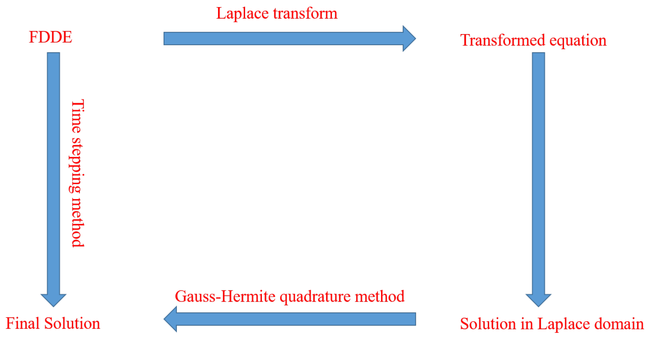
In this section, we describe the proposed numerical method for obtaining the solution of FDDEs. The main steps in our numerical method are as follows: (i) Using the Laplace transform, we reduce the considered FDDE to an algebraic equation; (ii) we solve the reduced equation in the Laplace domain; and (iii) finally, we utilize the inverse Laplace transform to recover the original problem’s solution. Since, the analytical inversion is difficult to compute, we instead use the numerical inversion technique. For the numerical inversion of the Laplace transform, we use the Gauss–Hermite quadrature method. The flowchart of the proposed numerical method is shown in Figure 1.

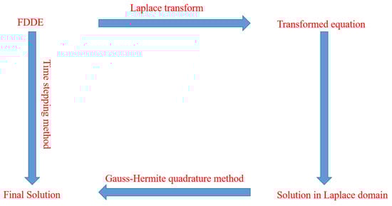
Figure 1. The flowchart of the proposed numerical method.

By applying the LT to (1)–(2), we obtain the following:

$$\mathcal{L}\left\{D_x^{\beta }y\left(x\right)\right\}=\mathcal{L}\{f\left(x\right)+A_{1}y\left(x\right)+A_{2}y(x-\chi )\},$$

$$\Rightarrow {\mu }^{\beta }\mathcal{L}\{y\left(x\right\}-{\mu }^{\beta -1}y\left(0\right)=\mathcal{L}\left\{f\left(x\right)\right\}+A_1\mathcal{L}\left\{y\left(x\right)\right\}+A_2\mathcal{L}\left\{y(x-\chi )\right\},$$

Then, using Theorem (2), we have

$$\Rightarrow {\mu }^{\beta }\widehat{y}\left(x\right)-{\mu }^{\beta -1}{\gamma }_1=\widehat{f}\left(\mu \right)+A_1\widehat{y}\left(\mu \right)+A_2\overline{\varrho }\left(\mu \right)+A_{2}exp(-\mu \chi )\widehat{y}\left(x\right),$$

or

$$\Rightarrow \left[{\mu }^{\beta }-A_1-A_{2}exp(-\mu \chi )\right]\widehat{y}\left(\mu \right)={\mu }^{\beta -1}{\gamma }_1+\widehat{f}\left(\mu \right)+A_2\overline{\varrho }\left(\mu \right).$$

(15)

Equation (15) can be simplified as

$$\widehat{y}\left(\mu \right)=\frac{{\mu }^{\beta -1}{\gamma }_1+\widehat{f}\left(\mu \right)+A_2\overline{\varrho }\left(\mu \right)}{{\mu }^{\beta }-A_1-A_{2}exp(-\mu \chi )}.$$

(16)

Taking the inverse LT of (16), we have

$$y\left(x\right)={\mathcal{L}}^{-1}\left\{\frac{{\mu }^{\beta -1}{\gamma }_1+\widehat{f}\left(\mu \right)+A_2\overline{\varrho }\left(\mu \right)}{{\mu }^{\beta }-A_1-A_{2}exp(-\mu \chi )}\right\}.$$

(17)

For numerous functions, the inverse LT in (17) cannot be inverted analytically using the techniques of complex analysis; therefore, numerical inversion methods are then used. The inverse LT in (17) is expressed as

$$y\left(x\right)=\frac{1}{2\pi i}{\int }_{\vartheta -i\infty }^{\vartheta +i\infty }{e}^{\mu x}\widehat{y}\left(\mu \right)d\mu =\frac{1}{2\pi i}{\int }_{\Gamma }{e}^{\mu x}\widehat{y}\left(\mu \right)d\mu .$$

(18)

Many numerical schemes for the evaluation of the integral (18) use quadrature rule. The function $\widehat{y}\left(\mu \right)$ is assumed to be analytic in the plane $\Re \left(\mu \right)>{\vartheta }_0$, with ${\vartheta }_0$ being the convergence abscissa. Typically, $\Gamma$ is selected to be the line $\Re \left(\mu \right)=\vartheta$ with $\vartheta >{\vartheta }_0.$ However, using Cauchy’s theorem, it is possible to deform this contour into a better one for computation. These deformations techniques provide efficient methods for analytical and numerical computation of (18). In numerical computation, we use the deformation, as the integral (18) is not suitable for quadrature on the line $\Re \left(\mu \right)=\vartheta$ due to the slow decaying transform function $\widehat{y}\left(\mu \right)$ as $\Im \left(\mu \right)\to \pm \infty$ and the highly oscillatory exponential factor $e^{\mu x}.$ The line $\Re \left(\mu \right)=\vartheta$ can be deformed to a contour which begins at $-\infty$ in the third quadrant and turns around all the singularities of $\widehat{y}\left(\mu \right)$ and ends at $+\infty$ in the second quadrant. On such a contour, the integrand decays rapidly due to the factor $\widehat{y}\left(\mu \right)$; furthermore, if the contour is smooth, this turns the problem in hand into a classical setting in which the trapezoidal converges very quickly. Fewer quadrature nodes and consequently less function evaluations are needed to achieve the desired accuracy. Such deformation is valid if the singularities of $\widehat{y}\left(\mu \right)$ and $|\widehat{y}\left(\mu \right)|\to 0$ as $\mu \to \infty$ [33] are all enclosed by the contour. For an effective numerical scheme, the implementation of two key factors must be considered: (i) integration contour and (ii) the quadrature-rule. The most famous methods in this area on the selection of optimal contour, the optimal values of parameters that define the contour and quadrature rule, are reported in [33,34,35,36,37]. In this article, the Gauss–Hermite quadrature (GHQ) rule is utilized as an alternative to the mid-point/trapezoidal rule.

Gauss–Hermite Quadrature Rule

The GHQ rule for a real valued function $h\left(t\right)$ defined on real line is given as [38]

$${\int }_{-\infty }^{\infty }{e}^{-t^2}h\left(t\right)dt\approx \sum _{\xi =1}^q{\eta }_{\xi }h\left(t_{\xi }\right).$$

(19)

The points $t_{\xi },$ are the roots of $H_{\nu }\left(t\right)$, the Hermite polynomial of degree $\nu$. The weights ${\eta }_{\xi },$ are determined uniquely by the property that if $H_{\nu }\left(t\right)$ is a polynomial not greater than $\nu -1,$ then the approximation sign can be replaced by an equal sign. For smooth functions $H_{\nu }\left(t\right)$, the convergence of Gauss–Hermite can be very fast. The following theorem, which was proven in [39,40], provides clarification for this statement.

Theorem 6.

The error in (19) can be expressed as

$$R_{\nu }\left(h\right)=\frac{1}{2\pi i}{\int }_{\Gamma }{\varphi }_{\nu }\left(\mu \right)h\left(\mu \right)d\mu ,$$

(20)

where

$${\varphi }_{\nu }\left(\mu \right)=\frac{Q_{\nu }\left(\mu \right)}{H_{\nu }\left(\mu \right)},Q_{\nu }\left(\mu \right)={\int }_{-\infty }^{\infty }{e}^{-t^2}\frac{H_{\nu }\left(t\right)}{\mu -t}dt.$$

(21)

The contour $\Gamma$ in (20) starts at $\mu =-\infty$, turns around the zeros of $H_{\nu }$, and ends at $\mu =\infty$, with $h\left(\mu \right)$ assumed to be analytic inside of it. The function $Q_{\nu }\left(\mu \right)$ in (21), known as a Hermite function of the second kind, decreases rapidly as $\left|\mu \right|\to \infty .$ Similarly, $H_{\nu }\left(\mu \right)$ rapidly increases, so the function ${\varphi }_{\nu }\left(\mu \right)$ in (20) can be fairly small, provided that the contour $\Gamma$ is significantly restricted by the growth or singularities of $h\left(\mu \right).$ High accuracy corresponds to singularities further from the real axis, and this fact can be used as follows. If we select $t=\varsigma x,\varsigma \in \mathbb{R},$ then

$${\int }_{-\infty }^{\infty }{e}^{-t^2}h\left(t\right)dt=\varsigma {\int }_{-\infty }^{\infty }{e}^{-{\varsigma }^2{x}^2}h\left(\varsigma x\right)dx=\varsigma {\int }_{-\infty }^{\infty }{e}^{-x^2}{e}^{x^2}{e}^{-{\varsigma }^2{x}^2}h\left(\varsigma x\right)dx,$$

(22)

Now, we can employ the rule (19) to the function $y\left(x\right)=e^{x^2(1-{\varsigma }^2)}h\left(\varsigma x\right).$ Then, $\widehat{y}\left(\mu \right)$ will have singularities farther from the x-axis as compared to the singularities of $h\left(\mu \right)$, and this may improve the accuracy. For evaluation of (18), the following contour is considered:

$$\Gamma :\mu =\vartheta {(1+i\zeta )}^2,-\infty <\zeta <\infty ,\vartheta >0.$$

(23)

The contour (23) intersects the $x-axis$ at $\mu =\vartheta$ and $y-axis$ at $\mu =\pm 2\vartheta i.$ Using (23), in (18), we obtain

$${\int }_{\Gamma }\widehat{y}\left(\mu \right)e^{\mu x}d\mu ={\int }_{-\infty }^{\infty }{e}^{\mu \left(\zeta \right)x}\widehat{y}\left(\mu \left(\zeta \right)\right){\mu }^{\prime }\left(\zeta \right)d\zeta ,$$

The scaling technique in (22) can be used via $\zeta =\varsigma \sigma$ as follows:

$$y\left(x\right)=\frac{\varsigma }{2\pi i}{\int }_{-\infty }^{\infty }{e}^{-{\sigma }^2}{e}^{{\sigma }^2+\mu \left(\varsigma \sigma \right)x}\widehat{y}\left(\mu \left(\varsigma \sigma \right)\right){\mu }^{\prime }\left(\varsigma \sigma \right)d\sigma ={\int }_{-\infty }^{\infty }{e}^{-{\sigma }^2}h\left(\sigma \right)d\sigma ,$$

or

$$y\left(x\right)={\int }_{-\infty }^{\infty }{e}^{-{\sigma }^2}h\left(\sigma \right)d\sigma ,$$

(24)

where

$$h\left(\sigma \right)=\frac{\varsigma }{2\pi i}{e}^{{\sigma }^2+\mu \left(\varsigma \sigma \right)x}\widehat{y}\left(\mu \left(\varsigma \sigma \right)\right){\mu }^{\prime }\left(\varsigma \sigma \right).$$

Now, employing the Gauss–Hermite quadrature to the right side of (24), we have

$$y_{App}\left(x\right)\approx 2Re\left\{\sum _{\xi =1}^p{\eta }_{\xi }h\left({\sigma }_{\xi }\right)\right\},$$

where the ${\sigma }_{\xi }$ are the positive roots of $H_{\nu }$, and for even $\nu$, we have $p=\nu /2$, and for odd $\nu$, we have $p=(\nu +1)/2$.

Theorem 7.

Suppose $\mathcal{C}: \mathcal{B}\to \mathcal{B}$ is a contraction mapping, $\mathcal{B}$ is the Banach space, and $0<\mathcal{S}<1$ is a constant; then, via the inverse LT, the solution can be expressed as follows:

$$y_k=\mathcal{C}\left(y_{k-1}\right),y_{k-1}=\sum _{j=1}^{k-1}{y}_j,k=1,2,3,...$$

and

$$y_k\in M_{\delta }\left(y\right)=\left\{\overline{y}\in \mathcal{B}:\parallel y-\overline{y}\parallel <\delta \right\},$$

$$\underset{k\to \infty }{lim}{y}_k=y,where{y}_0=y\left(0\right).$$

Proof. 

We use mathematical induction to obtain the desired result. For $k=1$, we obtain

$$\parallel y_1-y\parallel =\parallel \mathcal{C}{y}_0-\mathcal{C}y\parallel \le \mathcal{S}\parallel y_0-y\parallel .$$

Assuming the result is true for $k-1$, we have

$$\parallel y_{k-1}-y\parallel \le {\mathcal{S}}^{k-1}\parallel y_0-y\parallel .$$

(25)

Now

$$\parallel y_k-y\parallel =\parallel \mathcal{C}\left(y_{k-1}\right)-\mathcal{C}\left(y\right)\parallel \le \mathcal{S}\parallel y_{k-1}-y\parallel .$$

(26)

Using (25) and (26), we obtain

$$\parallel y_k-y\parallel \le \mathcal{S}{\mathcal{S}}^{k-1}\parallel y_0-y\parallel \le {\mathcal{S}}^k\delta <\delta .$$

which implies

$$y_k\in M_{\delta }\left(y\right).Alsok\to \infty ,{\mathcal{S}}^k\to 0.$$

Therefore,

$$\underset{k\to \infty }{lim}{y}_k=y.$$

which is the desired result. □

6. Application

In this section, we present the simulation results of the discussed numerical technique for fractional order DDEs. We have presented some numerical examples to show the efficiency of the proposed numerical method. Numerical experiments were performed with $\nu =20$ using MATLAB. The maximum absolute error $er{r}_{\infty }$ and root-mean-squared error $rm{s}_{err}$ were calculated for the considered problems. The error norms are defined as follows:

$$er{r}_{\infty }=\underset{1\le j\le n}{max}|y\left(x_j\right)-y_{App}\left(x_j\right)\left)\right|,$$

and

$$rm{s}_{err}=\sqrt{\frac{{\sum }_{j=1}^n{(y\left(x_j\right)-y_{App}\left(x_j\right))}^2}{n}},$$

where $y\left(x\right)$ and $y_{App}\left(x\right)$ denotes the exact and numerical solutions, respectively.

6.1. Example 1

Consider a FDDE

$$D_x^{\beta }y\left(x\right)=y(x-1)-y\left(x\right)+2x-1+\frac{\Gamma \left(3\right)}{\Gamma \left(\frac{5}{2}\right)}{x}^{\frac{3}{2}},x>0,$$

with delay and initial conditions

$$y\left(x\right)=x^2,-1\le x\le 0,$$

and

$$y\left(0\right)=0.$$

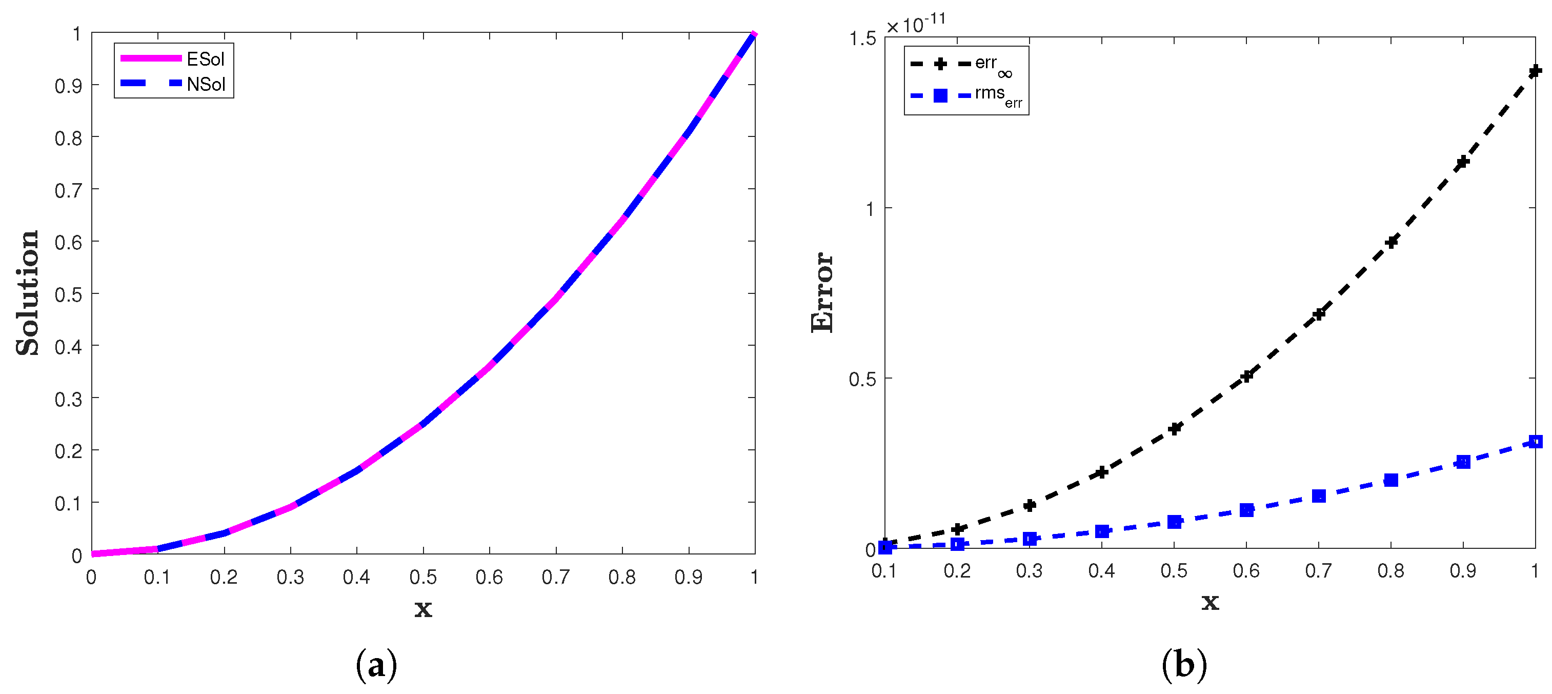
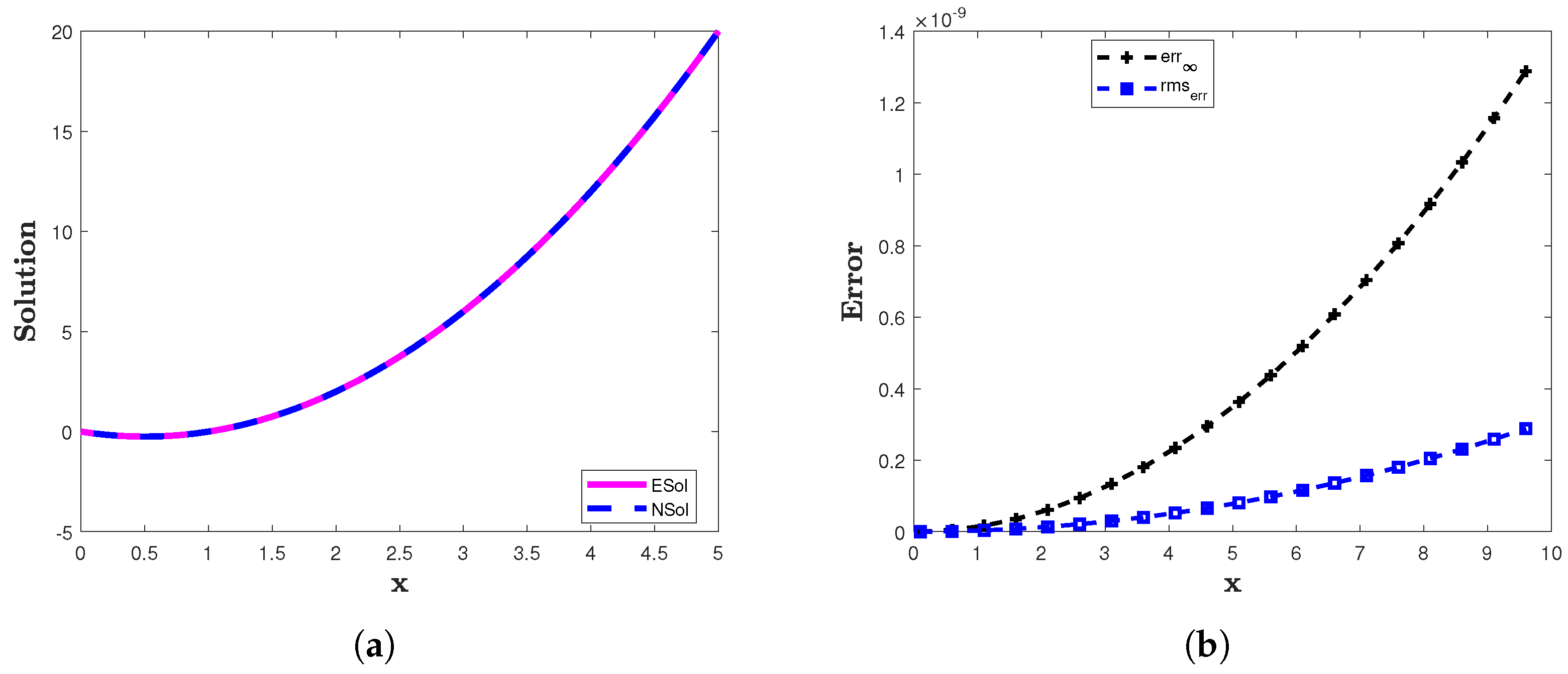
The analytic solution is $y\left(x\right)=x^2.$ The numerical solution of example 1 is obtained by employing GHQ method. The two error norms $er{r}_{\infty }$ and $rm{s}_{err}$ computed for example 1 are presented in Table 1 and Table 2. Numerical and exact solutions are plotted in Figure 2a. In Figure 2b, the $er{r}_{\infty }$ and $rm{s}_{err}$ are plotted for $x\in [0,1].$ In Table 1, we present the comparison of the errors of the proposed method with that of the fractional backward difference method [13]. Table 1 indicates that the solutions obtained by using the proposed method are closer to the exact solution when compared with the method of [13].

Table 1. The tabulated results of the $er{r}_{\infty }$ and $rm{s}_{err}$ computed by the suggested method for problem 1.

	x	${\mathit{err}}_{\mathit{\infty }}$	${\mathit{rms}}_{\mathit{err}}$	$\mathit{CPU}\left(\mathit{s}\right)$
	$0.1$	1.4014$\times {10}^{-13}$	3.1337$\times {10}^{-14}$	0.110374
	$0.3$	1.2613$\times {10}^{-12}$	2.8203$\times {10}^{-13}$	0.130806
	$0.5$	3.5035$\times {10}^{-12}$	7.8340$\times {10}^{-13}$	0.155005
	$0.7$	6.8680$\times {10}^{-12}$	1.5357$\times {10}^{-12}$	0.116574
	$0.9$	1.1351$\times {10}^{-11}$	2.5382$\times {10}^{-12}$	0.117173
	1	1.4015$\times {10}^{-11}$	3.1338$\times {10}^{-12}$	0.111987
[13]		9.8085$\times {10}^{-4}$

Table 2. Numerical solution of example 1.

x	Exact Solution	Proposed Method	[16]
0.2	0.04	0.04	0.04
0.4	0.16	0.16	0.16
0.6	0.36	0.36	0.36
0.8	0.64	0.64	0.64
1.0	1	1	1.028
1.2	1.44	1.44	1.4692
1.4	1.96	1.96	2.0175
1.6	2.56	2.56	2.6861
1.8	3.24	3.24	3.44
2	4	4	4.2456

Figure 2. (a) The approximate (NSol) and analytic (ESol) solutions of example 1. (b) The $er{r}_{\infty }$ and $rm{s}_{err}$ of the proposed method for example 1 with $x\in [0,1]$ and $\beta =0.5$.

6.2. Example 2

Consider a FDDE

$$D_x^{\beta }y\left(x\right)=y(x-1)-y\left(x\right)+1-3x+3x^2+\frac{20t^{3-\beta }}{9\Gamma (3-\beta )},x>0,$$

with delay and initial conditions

$$y\left(x\right)=x^3,-1\le x\le 0,$$

and

$$y\left(0\right)=0.$$

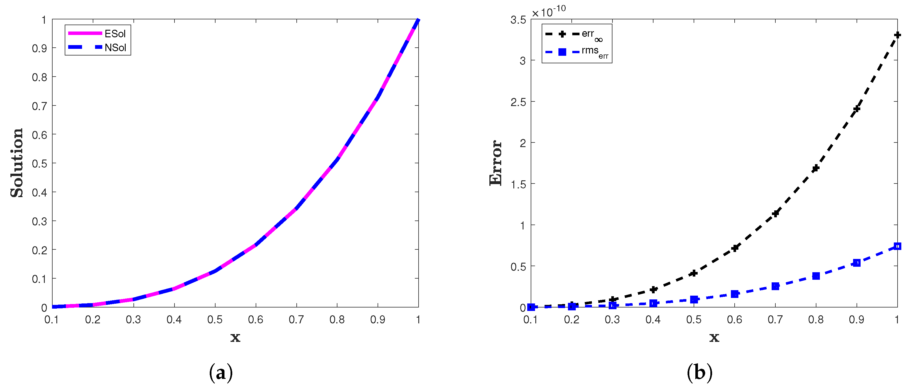
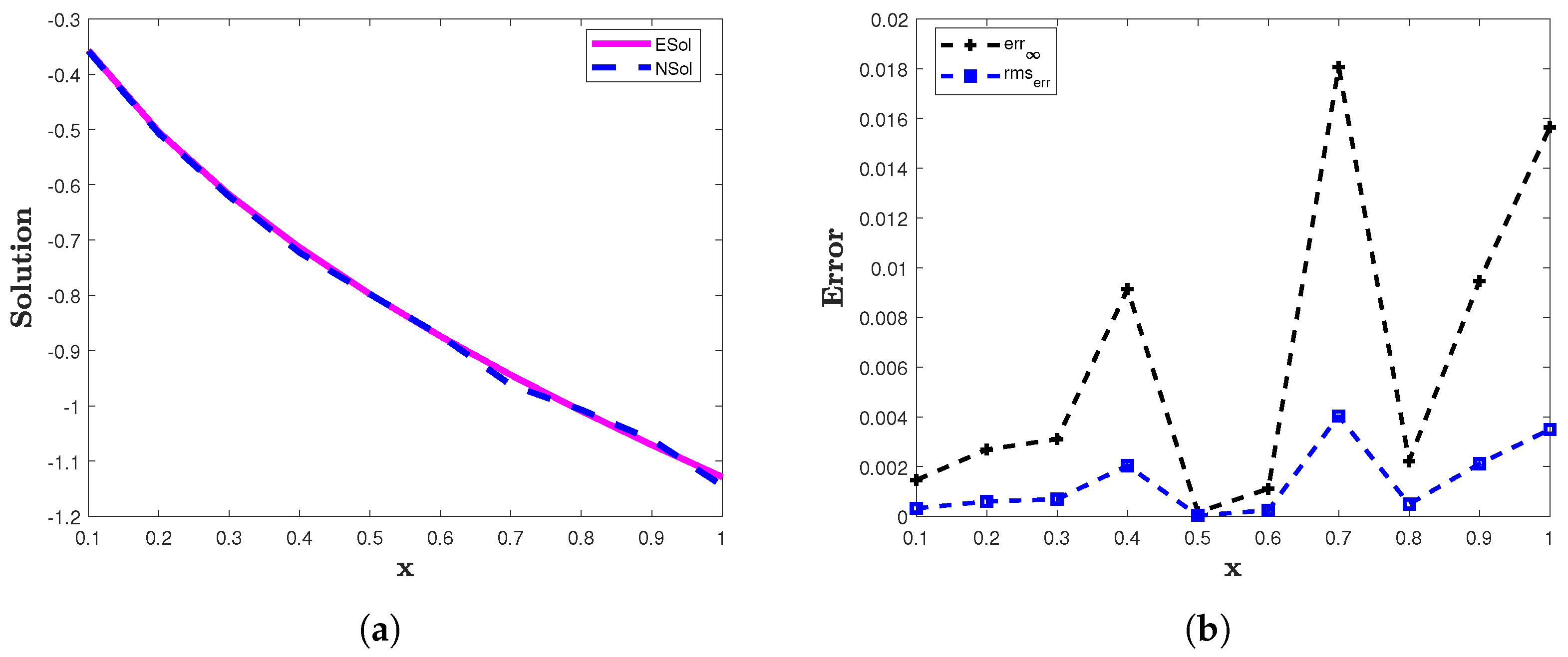
The analytic solution is $y\left(x\right)=x^3.$ The two error norms $er{r}_{\infty }$ and $rm{s}_{err}$ computed for example 2 are presented in Table 3. In Figure 3a, we illustrate a comparison between the analytic solution and the approximate solution obtained by the proposed method. In Figure 3b, we graphically illustrate the comparison of the $er{r}_{\infty }$ and $rm{s}_{err}$ for $x\in [0,1].$ In Table 3, we present a comparison of the errors of the proposed method and the fractional backward difference method [13]. For this problem, the proposed method also produces accurate results.

Table 3. The tabulated results of the $er{r}_{\infty }$ and $rm{s}_{err}$ computed by the suggested method for example 2.

	x	${\mathit{err}}_{\mathit{\infty }}$	${\mathit{rms}}_{\mathit{err}}$	$\mathit{CPU}\left(\mathit{s}\right)$
	$0.1$	3.3054$\times {10}^{-13}$	7.3911$\times {10}^{-14}$	0.147631
	$0.3$	8.9247$\times {10}^{-12}$	1.9956$\times {10}^{-12}$	0.118002
	$0.5$	4.1318$\times {10}^{-11}$	9.2389$\times {10}^{-12}$	0.118522
	$0.7$	1.1338$\times {10}^{-10}$	2.5352$\times {10}^{-11}$	0.112424
	$0.9$	2.4097$\times {10}^{-10}$	5.3881$\times {10}^{-11}$	0.105683
	1	3.3054$\times {10}^{-10}$	7.3912$\times {10}^{-11}$	0.101965
[13]		1.4487$\times {10}^{-3}$

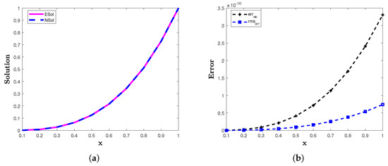
Figure 3. (a) The approximate (NSol) and analytic (ESol) solutions of example 2. (b) The $er{r}_{\infty }$ and $rm{s}_{err}$ of the proposed method for example 2 with $x\in [0,1]$ and $\beta =0.3$.

6.3. Example 3

Consider a FDDE

$$D_x^{\beta }y\left(x\right)=\frac{2}{\Gamma (3-\beta )}{x}^{2-\beta }-\frac{1}{\Gamma (2-\beta )}{x}^{1-\beta }+2\chi x-{\chi }^2-\chi -y\left(x\right)+y(x-\chi ),0<\beta \le 1,$$

with delay and initial conditions

$$y\left(x\right)=0,-1\le x\le 0,$$

and

$$y\left(0\right)=0.$$

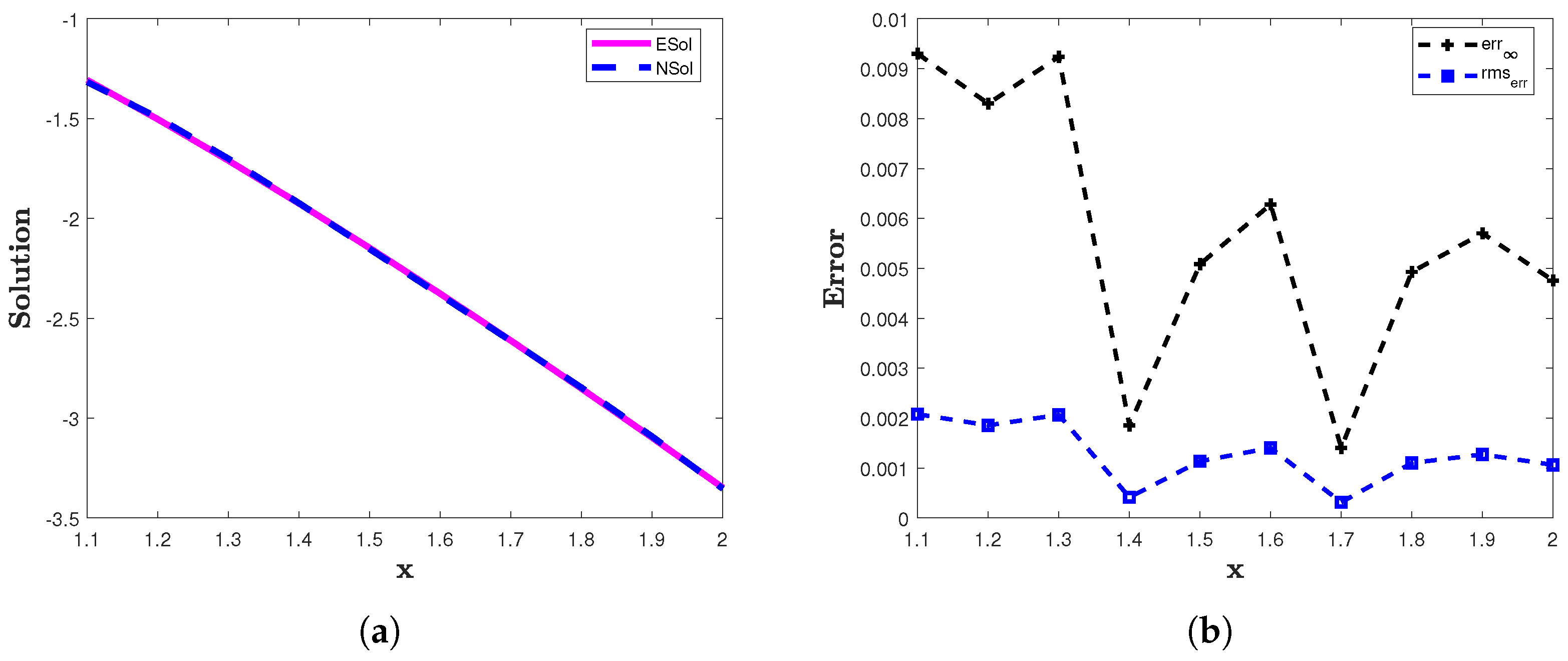
The analytic solution is $y\left(x\right)=x^2-x.$ This example is solved using the suggested scheme with constant and time-varying delay. The two error norms $er{r}_{\infty }$ and $rm{s}_{err}$ computed for example 3 are presented in Table 4. In Table 4, we compare the errors obtained by using our suggested numerical scheme with those results obtained using the Adams–Bashforth–Moulton method [41]. The results show that the suggested scheme produces accurate results. In Figure 4a, a comparison between the analytic solution and the approximate solution obtained by the proposed method is illustrated. In Figure 4b, a comparison between the $er{r}_{\infty }$ and $rm{s}_{err}$ is graphically illustrated for $x\in [0,1].$ The results presented in graphs and Table 4 suggest that this technique can be used in the simulation of high order FDDEs.

Table 4. The tabulated results of the $er{r}_{\infty }$ and $rm{s}_{err}$ computed by the suggested method for example 3 with different $\chi$ and $\beta$.

	x	${\mathit{err}}_{\mathit{\infty }}$	${\mathit{rms}}_{\mathit{err}}$	$\mathit{CPU}\left(\mathit{s}\right)$	[41]
$\chi =0.1$	5	3.3402$\times {10}^{-04}$	7.4690$\times {10}^{-05}$	0.130427	6.20$\times {10}^{-03}$
$\beta =0.2$	10	1.8837$\times {10}^{-04}$	4.2120$\times {10}^{-05}$	0.102818	1.34$\times {10}^{-02}$
	50	5.1148$\times {10}^{-05}$	1.1437$\times {10}^{-05}$	0.122529	9.90$\times {10}^{-02}$
$\chi =0.1$	5	3.9423$\times {10}^{-03}$	8.8153$\times {10}^{-04}$	0.106599	3.30$\times {10}^{-03}$
$\beta =0.9$	10	3.6955$\times {10}^{-03}$	8.2633$\times {10}^{-04}$	0.109374	3.10$\times {10}^{-03}$
	50	3.1777$\times {10}^{-03}$	7.1056$\times {10}^{-04}$	0.124888	2.30$\times {10}^{-03}$
$\chi =0.01e^{-x}$	5	4.8500$\times {10}^{-10}$	1.0845$\times {10}^{-10}$	0.104304	7.40$\times {10}^{-03}$
$\beta =0.2$	10	1.3979$\times {10}^{-09}$	3.1258$\times {10}^{-10}$	0.100498	8.20$\times {10}^{-03}$
	50	3.5020$\times {10}^{-08}$	7.8307$\times {10}^{-09}$	0.120393	5.20$\times {10}^{-03}$
$\chi =0.01e^{-x}$	5	2.1570$\times {10}^{-09}$	4.8231$\times {10}^{-10}$	0.103760	1.0$\times {10}^{-03}$
$\beta =0.9$	10	1.3979$\times {10}^{-09}$	3.1259$\times {10}^{-10}$	0.104422	4.711$\times {10}^{-04}$
	50	3.5019$\times {10}^{-08}$	7.8305$\times {10}^{-09}$	0.105549	7.030$\times {10}^{-04}$

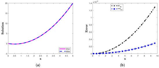
Figure 4. (a) The approximate (NSol) and analytic (ESol) solutions of example 3. (b) The $er{r}_{\infty }$ and $rm{s}_{err}$ of the proposed method for example 3 with $x\in [0,10]$ and $\beta =0.9$.

6.4. Example 4

Consider a FDDE

$$D_x^{\beta }y\left(x\right)=y(x-1)-x,0<\beta \le 1,$$

with delay and initial conditions

$$y\left(x\right)=x,-1\le x\le 0,$$

and

$$y\left(0\right)=0.$$

The analytic solution is

$$y\left(x\right)=\frac{-2}{\Gamma \left(0.5\right)}\sqrt{x},\mathrm{if}0\le x<1,$$

and

$$y\left(x\right)=\frac{2}{\sqrt{\pi }}\left(\sqrt{x-1}-\sqrt{x}\right)+1-x-\frac{2\sqrt{x-1}(1+2x)}{3\sqrt{\pi }},\mathrm{if}1\le x<2.$$

The two error norms $er{r}_{\infty }$ and $rm{s}_{err}$ computed for example 4 are presented in Table 5. The graphical demonstration of the analytic solution and the approximate solution obtained by the proposed numerical technique for $0\le x<1$ are presented in Figure 5a and for $1\le x<2$ in Figure 6a. The $er{r}_{\infty }$ and $rm{s}_{err}$ are plotted for $x\in [0,1]$ in Figure 5b and for $x\in [1,2]$ in Figure 6b. The computed solution of the proposed scheme is compared with the solution of [13,16] in Table 5 and Table 6. From these results, we can see that the proposed numerical method provides accurate results for wide intervals of $x.$

Table 5. The tabulated results of the $er{r}_{\infty }$ and $rm{s}_{err}$ computed by the suggested method for example 4.

	x	${\mathit{err}}_{\mathit{\infty }}$	${\mathit{rms}}_{\mathit{err}}$	$\mathit{CPU}\left(\mathit{s}\right)$
	$0.1$	1.4630$\times {10}^{-3}$	3.2714$\times {10}^{-4}$	0.124060
	$0.3$	3.1078$\times {10}^{-3}$	6.9493$\times {10}^{-4}$	0.125002
	$0.5$	1.6985$\times {10}^{-4}$	3.7980$\times {10}^{-5}$	0.126084
	$0.7$	1.8069$\times {10}^{-2}$	4.0404$\times {10}^{-3}$	0.104953
	$0.9$	9.4689$\times {10}^{-3}$	2.1173$\times {10}^{-3}$	0.130307
	1	1.5646$\times {10}^{-2}$	3.4985$\times {10}^{-3}$	0.118086
	$1.1$	9.2996$\times {10}^{-3}$	2.0794$\times {10}^{-3}$	0.125332
	$1.3$	9.2384$\times {10}^{-3}$	2.0658$\times {10}^{-3}$	0.105014
	$1.5$	5.0839$\times {10}^{-3}$	1.1368$\times {10}^{-3}$	0.104054
	$1.7$	1.4055$\times {10}^{-3}$	3.1429$\times {10}^{-4}$	0.103424
	$1.9$	5.7012$\times {10}^{-3}$	1.2748$\times {10}^{-3}$	0.111321
	2	4.7573$\times {10}^{-3}$	1.0638$\times {10}^{-3}$	0.106843
[13]		9.626$\times {10}^{-3}$

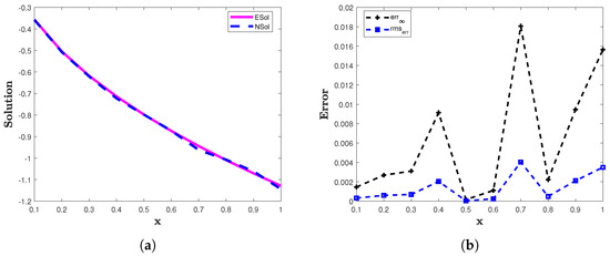
Figure 5. (a) The approximate(NSol) and analytic (ESol) solutions of example 4 for $x\in [0,1]$. (b) The $er{r}_{\infty }$ and $rm{s}_{err}$ of the proposed method for example 4 with $x\in [0,1]$ and $\beta =0.5$.

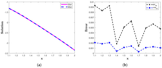
Figure 6. (a) The numerical (NSol) and exact (ESol) solutions of example 4 for $x\in [1,2]$. (b) The $er{r}_{\infty }$ and $rm{s}_{err}$ of the proposed method for example 4 with $x\in [1,2]$ and $\beta =0.5$.

Table 6. Numerical solution of example 4.

x	Exact Solution	Proposed Method	[16]
$0.20$	$-0.5046$	$-0.5073$	$-0.5044$
$0.40$	$-0.7136$	$-0.7228$	$-0.7142$
$0.60$	$-0.8740$	$-0.8729$	$-0.8736$
$0.80$	$-1.0093$	$-1.0070$	$-1.0096$
$1.00$	$-1.1284$	$-1.1440$	$-1.1427$
$1.20$	$-1.5034$	$-1.4951$	$-1.4637$
$1.40$	$-1.9254$	$-1.9236$	$-1.8815$
$1.60$	$-2.3769$	$-2.3832$	$-2.4091$
$1.80$	$-2.8521$	$-2.8472$	$-3.0060$
$2.00$	$-3.3480$	$-3.3528$	$-3.6385$

7. Conclusions

In this article, we first examine the existence of solutions to linear FDDEs. Then, we discuss the UH stability of the considered FDDEs. We examine the numerical solution of the FDDEs using the Laplace transform and Gauss–Hermite quadrature method. Our main objective was to develop an efficient numerical method for solving this class of equations, which frequently arise in numerous fields such as signal processing, control theory, and biological systems. To find out if the suggested numerical technique supports the stability of the problem considered, we considered numerical examples with constant and time-varying delay. The following conclusions can be drawn from the results presented in Tables and Figures.

• The error is very small in our approximations.
• The proposed method produces accurate results in a very short computation time.
• The results demonstrate that the proposed method can solve FDDEs efficiently.

Future research could focus on enhancing the stability through numerical methods and investigating the adaptability of this method to more complex and higher-dimensional problems.

References

- Alyobi, S.; Jan, R. Qualitative and quantitative analysis of fractional dynamics of infectious diseases with control measures. Fractal Fract. 2003, 7, 400. [Google Scholar] [CrossRef]
- Miller, K.S.; Ross, B. An Introduction to the Fractional Calculus and Fractional Differential Equations; John Wiley & Sons: New York, NY, USA, 1993. [Google Scholar]
- Kilbas, A.A.; Srivastava, H.M.; Trujillo, J.J. Theory and Applications of Fractional Differential Equations; Elsevier: Amsterdam, The Netherlands, 2006; Volume 204. [Google Scholar]
- Kamran; Shah, F.A.; Aly, W.H.F.; Aksoy, H.; Alotaibi, F.M.; Mahariq, I. Numerical Inverse Laplace Transform Methods for Advection-Diffusion Problems. Symmetry 2022, 14, 2544. [Google Scholar] [CrossRef]
- Atangana, A.; Gómez-Aguilar, J.F. Hyperchaotic behaviour obtained via a nonlocal operator with exponential decay and Mittag-Leffler laws. Chaos Solitons Fractals 2017, 102, 285–294. [Google Scholar] [CrossRef]
- Tang, T.Q.; Shah, Z.; Bonyah, E.; Jan, R.; Shutaywi, M.; Alreshidi, N. Modeling and analysis of breast cancer with adverse reactions of chemotherapy treatment through fractional derivative. In Computational and Mathematical Methods in Medicine; John Wiley & Sons: New York, NY, USA, 2022. [Google Scholar]
- Jan, R.; Boulaaras, S. Analysis of fractional-order dynamics of dengue infection with non-linear incidence functions. Trans. Inst. Meas. Control. 2022, 44, 2630–2641. [Google Scholar] [CrossRef]
- Tang, T.Q.; Shah, Z.; Jan, R.; Alzahrani, E. Modeling the dynamics of tumor–immune cells interactions via fractional calculus. Eur. Phys. J. Plus 2022, 137, 367. [Google Scholar] [CrossRef]
- Cooke, K.; Kuang, Y.; Li, B. Analyses of an antiviral immune response model with time delays. Can. Appl. Math. Q. 1998, 6, 321–354. [Google Scholar]
- Cooke, K.; Van den Driessche, P.; Zou, X. Interaction of maturation delay and nonlinear birth in population and epidemic models. J. Math. Biol. 1999, 39, 332–352. [Google Scholar] [CrossRef] [PubMed]
- Nelson, P.W.; Murray, J.D.; Perelson, A.S. A model of HIV-1 pathogenesis that includes an intracellular delay. Math. Biosci. 2000, 163, 201–215. [Google Scholar] [CrossRef] [PubMed]
- Vielle, B.; Chauvet, G. Delay equation analysis of human respiratory stability. Math. Biosci. 1998, 152, 105–122. [Google Scholar] [CrossRef]
- Morgado, M.L.; Ford, N.J.; Lima, P.M. Analysis and numerical methods for fractional differential equations with delay. J. Comput. Appl. Math. 2013, 252, 159–168. [Google Scholar] [CrossRef]
- Moghaddam, B.P.; Mostaghim, Z.S. A numerical method based on finite difference for solving fractional delay differential equations. J. Taibah Univ. Sci. 2013, 7, 120–127. [Google Scholar] [CrossRef]
- Jhinga, A.; Daftardar-Gejji, V. A new numerical method for solving fractional delay differential equations. Comput. Appl. Math. 2019, 38, 1–18. [Google Scholar] [CrossRef]
- Muthukumar, P.; Ganesh Priya, B. Numerical solution of fractional delay differential equation by shifted Jacobi polynomials. Int. J. Comput. Math. 2017, 94, 471–492. [Google Scholar] [CrossRef]
- Chishti, F.; Hanif, F.; Shams, R. A Comparative Study on Solution Methods for Fractional order Delay Differential Equations and its Applications. Math. Sci. Appl. 2023, 2, 1–13. [Google Scholar]
- Izadi, M.; Yüzbaşi, Ş.; Adel, W. A new Chelyshkov matrix method to solve linear and nonlinear fractional delay differential equations with error analysis. Math. Sci. 2023, 17, 267–284. [Google Scholar] [CrossRef]
- Naseem, T.; Zeb, A.A.; Sohail, M. Reduce Differential Transform Method for Analytical Approximation of Fractional Delay Differential Equation. Int. J. Emerg. Multidiscip. Math. 2022, 1, 104–123. [Google Scholar] [CrossRef]
- Rebenda, J.; Šmarda, Z. A differential transformation approach for solving functional differential equations with multiple delays. Commun. Nonlinear Sci. Numer. Simul. 2017, 48, 246–257. [Google Scholar] [CrossRef]
- Li, S.; Khan, S.U.; Riaz, M.B.; AlQahtani, S.A.; Alamri, A.M. Numerical simulation of a fractional stochastic delay differential equations using spectral scheme: A comprehensive stability analysis. Sci. Rep. 2024, 14, 6930. [Google Scholar] [CrossRef] [PubMed]
- Shah, K.; Sher, M.; Sarwar, M.; Abdeljawad, T. Analysis of a nonlinear problem involving discrete and proportional delay with application to Houseflies model. Aims Math. 2024, 9, 7321–7339. [Google Scholar] [CrossRef]
- Sher, M.; Shah, K.; Rassias, J. On qualitative theory of fractional order delay evolution equation via the prior estimate method. Math. Methods Appl. Sci. 2020, 43, 6464–6475. [Google Scholar] [CrossRef]
- Yao, Z.; Yang, Z.; Fu, Y.; Liu, S. Stability analysis of fractional-order differential equations with multiple delays: The 1<α<2 case. Chin. J. Phys. 2024, 89, 951–963. [Google Scholar]
- Kamal, R.; Kamran; Alzahrani, S.M.; Alzahrani, T. A Hybrid Local Radial Basis Function Method for the Numerical Modeling of Mixed Diffusion and Wave-Diffusion Equations of Fractional Order Using Caputo’s Derivatives. Fractal Fract. 2023, 7, 381. [Google Scholar] [CrossRef]
- Kamran; Kamal, R.; Rahmat, G.; Shah, K. On the numerical approximation of three-dimensional time fractional convection-diffusion equations. Math. Probl. Eng. 2021, 2021, 4640467. [Google Scholar]
- Kamran; Ali, A.; Gómez-Aguilar, J.F. A transform based local RBF method for 2D linear PDE with Caputo–Fabrizio derivative. Comptes Rendus. Mathématique 2020, 358, 831–842. [Google Scholar]
- López-Fernández, M.; Palencia, C. On the numerical inversion of the Laplace transform of certain holomorphic mappings. Appl. Numer. Math. 2004, 51, 289–303. [Google Scholar] [CrossRef]
- Kamran; Khan, S.U.; Haque, S.; Mlaiki, N. On the Approximation of Fractional-Order Differential Equations Using Laplace Transform and Weeks Method. Symmetry 2023, 15, 1214. [Google Scholar]
- Cimen, E.; Uncu, S. On the solution of the delay differential equation via Laplace transform. Commun. Math. Appl. 2020, 11, 379. [Google Scholar]
- Webb, J. Initial value problems for Caputo fractional equations with singular nonlinearities. Electron. J. Differ. Equ. 2019, 2019, 1–32. [Google Scholar]
- Agarwal, R.P.; Meehan, M.; O’regan, D. Fixed Point Theory and Applications; Cambridge University Press: Cambridge, UK, 2001; p. 141. [Google Scholar]
- Talbot, A. The accurate numerical inversion of Laplace transforms. Ima J. Appl. Math. 1979, 23, 97–120. [Google Scholar] [CrossRef]
- Trefethen, L.N.; Weideman, J.A.C. The exponentially convergent trapezoidal rule. Siam Rev. 2014, 56, 385–458. [Google Scholar] [CrossRef]
- Weideman, J.; Trefethen, L. Parabolic and hyperbolic contours for computing the Bromwich integral. Math. Comput. 2007, 76, 1341–1356. [Google Scholar] [CrossRef]
- Kamran; Gul, U.; Alotaibi, F.M.; Shah, K.; Abdeljawad, T. Computational approach for differential equations with local and nonlocal fractional-order differential operators. J. Math. 2023, 2023, 6542787. [Google Scholar]
- Kamran; Ahmad, S.; Shah, K.; Abdeljawad, T.; Abdalla, B. On the Approximation of Fractal-Fractional Differential Equations Using Numerical Inverse Laplace Transform Methods. Cmes-Comput. Model. Eng. Sci. 2023, 135, 2743–2765. [Google Scholar]
- Weideman, J.A.C. Gauss–Hermite quadrature for the Bromwich integral. Siam J. Numer. Anal. 2019, 57, 2200–2216. [Google Scholar] [CrossRef]
- Barrett, W. Convergence properties of Gaussian quadrature formulae. Comput. J. 1961, 3, 272–277. [Google Scholar] [CrossRef]
- Takahasi, H.; Mori, M. Estimation of errors in the numerical quadrature of analytic functions. Appl. Anal. 1971, 1, 201–229. [Google Scholar] [CrossRef]
- Wang, Z. A numerical method for delayed fractional-order differential equations. J. Appl. Math. 2013, 2013, 256071. [Google Scholar] [CrossRef]
Disclaimer/Publisher’s Note: The statements, opinions and data contained in all publications are solely those of the individual author(s) and contributor(s) and not of MDPI and/or the editor(s). MDPI and/or the editor(s) disclaim responsibility for any injury to people or property resulting from any ideas, methods, instructions or products referred to in the content. |
© 2024 by the authors. Licensee MDPI, Basel, Switzerland. This article is an open access article distributed under the terms and conditions of the Creative Commons Attribution (CC BY) license (https://creativecommons.org/licenses/by/4.0/).