A Dynamic Surrogate-Assisted Hybrid Breeding Algorithm for High-Dimensional Imbalanced Feature Selection

Abstract

With the growing complexity of high-dimensional imbalanced datasets in critical fields such as medical diagnosis and bioinformatics, feature selection has become essential to reduce computational costs, alleviate model bias, and improve classification performance. DS-IHBO, a dynamic surrogate-assisted feature selection algorithm integrating relevance-based redundant feature filtering and an improved hybrid breeding algorithm, is presented in this paper. Departing from traditional surrogate-assisted approaches that use static approximations, DS-IHBO employs a dynamic surrogate switching mechanism capable of adapting to diverse data distributions and imbalance ratios through multiple surrogate units built via clustering. It enhances the hybrid breeding algorithm with asymmetric stratified population initialization, adaptive differential operators, and t-distribution mutation strategies to strengthen its global exploration and convergence accuracy. Tests on 12 real-world imbalanced datasets (4–98% imbalance) show that DS-IHBO achieves a 3.48% improvement in accuracy, a 4.80% improvement in F1 score, and an 83.85% reduction in computational time compared with leading methods. These results demonstrate its effectiveness for high-dimensional imbalanced feature selection and strong potential for real-world applications.

1. Introduction

With the rapid development of information technology and the advent of the big data era, various types of data now exhibit characteristics of high dimensionality, complexity, and diversity. Among these types of data, high-dimensional imbalanced data are commonly found in numerous fields, including financial fraud detection [1], medical diagnosis [2], bioinformatics [3], and intrusion detection [4]. Such data possess distinct properties in terms of sample size and feature dimensionality. For instance, credit card fraud detection datasets contain significantly fewer fraudulent samples than normal transactions, and these transaction records often exhibit highly dimensional feature spaces [1]. Similarly, in the medical field, diagnostic data for rare diseases typically include few samples but numerous features [2]. These data not only fail to effectively convey class label information but also provide misleading signals for subsequent modeling.

Feature selection (FS) is a crucial dimensionality-reduction technique that has been widely adopted across various domains, such as natural language processing and computer vision [5,6,7]. The FS workflow typically involves three main steps. First, a subset of features is selected. Second, this subset is evaluated using an evaluation function. Third, the selection is iteratively refined until a termination condition is met or a maximum number of iterations is achieved [8]. FS constitutes a quintessential NP-hard combinatorial problem, where the solution space grows exponentially with respect to the dimensionality of features. Some features that appear to have weak correlations with the target individually might contribute significantly to classification tasks when combined in specific ways. When existing FS methods are applied to high-dimensional imbalanced datasets, several issues arise in terms of feature evaluation metrics. Some methods have moved beyond traditional class-related indicators, instead assessing feature performance based on distributional differences across classes [9,10]. However, they still tend to incur FS bias, lack a dynamic trade-off mechanism, overlook the synergistic effects among features, and exhibit substantially increased computational complexity.

Evolutionary algorithms (EAs), including particle swarm optimization (PSO) [11], genetic algorithm (GA) [12], and other advanced variants [13,14,15], have been widely applied across numerous disciplines. This is due to their capability of optimizing non-differentiable and non-continuous objective functions. Sadeeq et al. [16] proposed Cauchy Artificial Rabbits Optimization (CARO) to improve ARO’s search ability in constrained environments and solve complex constrained optimization problems in power system engineering. Sun et al. [17] developed the three-stage FSUHO approach to find optimal feature subsets in high-dimensional data and address overlooked feature–feature/feature–class interactions. Among these EAs, the hybrid breeding optimization algorithm (HBO) [18] stands out due to its powerful search ability and co-evolution mechanism. Drawing on hybrid vigor theory, which implies a form of symmetric enhancement between parental traits, HBO has been successfully applied to intrusion detection [19], FS [20], and bandwidth selection [21] problems. Nevertheless, when applied to high-dimensional imbalanced FS problems, HBO and its variants still experience slow convergence rates and limited robustness, underscoring the need for improved symmetry between model capacity and problem complexity.

Surrogate-assisted EAs have demonstrated remarkable effectiveness in computationally intensive applications, and their integration into FS provides a promising direction for reducing computational costs in high-dimensional scenarios. Brownlee et al. [22] employed a Markov network as a surrogate model and adopted GA to search within this network. Chen et al. [23] developed a PSO-based FS approach using correlation-guided updating and surrogate-based particle selection to enhance search efficiency. Nguyen et al. [24] proposed a surrogate-assisted FS method that constructs a representative sample set from the original data to reduce computational cost. Song et al. [25] introduced a cooperative feature and sample grouping strategy combined with surrogate-assisted PSO to tackle high-dimensional FS. These methods can be broadly categorized into two groups according to their surrogate model construction strategies: the first two focus on building surrogate models for the objective function (i.e., fitness), which are referred to as objective regression surrogates; the latter two utilize a small number of representative samples as a substitute for the entire dataset, and are thus termed sample surrogates. In turn, these findings provide solid empirical and methodological support for the successful application of surrogate models in FS. However, most surrogate models still lack the capacity to capture high-dimensional nonlinear feature interactions, especially the weak signals from minority classes, which consequently degrade the classification performance of the resulting feature subsets.

To address these drawbacks, this paper investigates an improved HBO (IHBO) algorithm based on filtering and dynamic surrogate-assisted strategies, called DS-IHBO, for high-dimensional imbalanced FS in classification problems. The main contributions of this paper are as follows:

• IHBO, a binary variant of HBO, is developed through the incorporation of hierarchical population initialization, t-distribution mutation disturbance, and an adaptive difference operator selection strategy into HBO to enhance its performance. These improvements enable the algorithm to escape the local optimum and improve exploration in high-dimensional spaces, leading to a significant boost in its global search and optimization performance.
• DS-IHBO, a hybrid FS method, is proposed. In this method, irrelevant features are removed based on an importance index; IHBO is utilized for global optimization, and a fast dynamic surrogate-assisted strategy is incorporated. The original dataset is used to evaluate the fitness of the global optimal solution in each iteration, while the surrogate unit is dynamically switched to assess other solutions. This design makes it particularly well-suited for real-world applications such as disease detection in medical scenes.
• The proposed methods are validated on twelve datasets. The experimental results demonstrate that the proposed approach significantly outperforms six state-of-the-art techniques in key classification performance metrics and computational cost, showcasing its efficacy in handling high-dimensional, imbalanced, and complex data.

The structure of this paper is organized as follows. Section 2 presents the related work and foundational problem definitions. Section 3 details the proposed methodology. Experimental validation of the approach is provided in Section 4, while Section 5 concludes with a conclusion and discussion.

2. Related Work and Foundational Problem Definitions

This section focuses on reviewing FS methods, introducing the foundational HBO algorithm, and defining symmetric uncertainty.

2.1. FS Methods Review

(i) Classical FS methods: classical FS methods are divided into traditional FS and EAs-based FS methods. The working principles, advantages, and disadvantages of these two methods are shown in Table 1. Among these, EA-based methods have still remained a focus of attention in recent years [26,27,28]. Pan et al. [29] developed a binary version of the Rafflesia Optimization Algorithm (ROA) by using transfer functions for binarization and a parallel strategy to enhance convergence speed and global exploration capability. Li et al. [30] tackled the oversimplification in current task generation approaches by employing diverse filtering techniques to produce heterogeneous tasks, subsequently adapting a competitive swarm optimization (CSO) algorithm to effectively solve these tasks via knowledge transfer mechanisms. Building on the above work, EA-based FS methods remain viable but face significant challenges in adapting to increasingly complex scenarios (e.g., slow search in high-dimensional spaces, failure to identify truly discriminative subsets under class imbalance). Their rational integration with other FS methods (e.g., filter methods, clustering, surrogate-assisted techniques) is required to unlock their full potential.

Table 1. Classical FS methods.

Category	Branch	Process	Advantage	Disadvantage
Traditional FS [31]	Filter method	Evaluate feature relevance redundancy via statistical ranking measures	Suitable for high-dimensional data	Hard to determine optimal feature number and remove redundancies
	Wrapper method	Search optimal feature subset by evaluating subset performance with a classifier	Good at handling nonlinear feature interactions dependencies	High computational cost, prone to overfitting [32]
	Embedded method	Integrate FS into learning algorithm training	Low computational complexity	Classification accuracy depends on classifier, poor robustness [33]
EAs-based FS	PSO, GWO-based FS et al. [34,35]	EA-based FS encodes subsets, evaluates fitness, optimizes, outputs optimal ones on termination	Strong global search capability, clear goal orientation	High computational cost, parameter sensitivity

(ii) Surrogate-assisted FS methods: This category is pivotal for alleviating the high computational cost of EAs-based FS and is classified into sample surrogates and objective regression surrogates with distinct technical paths and trade-offs (see Table 2). Sample surrogates reduce computation by building surrogate units from representative data subsets, further divided into static and dynamic types. Static sample surrogates use a fixed set of representative instances, yet their static nature causes inaccuracies when data distributions shift during iterative FS. Dynamic sample surrogates enhance robustness via dynamic surrogate unit switching/updating, though at the cost of complex sampling and management design. Objective regression surrogates approximate fitness functions using models like Kriging or SVM; however, models such as SVM, tailored for continuous spaces, poorly adapt to discrete FS. Sample surrogates generally offer higher prediction accuracy than objective regression surrogates, which are more computationally efficient. Given that FS is a discrete optimization task, sample surrogates are better suited, while objective regression surrogates struggle with discrete feature spaces. Thus, this study focuses on designing sample surrogates and their dynamic management for discrete FS.

Table 2. Surrogate-assisted FS methods.

Category	Branch	Examples	Process	Ad. and DisAd.
Sample surrogate	Static sample surrogate	[24]	Select a small number of instances to build a surrogate training set and combine with sampling local search	High classification accuracy, adapts to high-dimensional data; difficult to adapt to data distribution changes, accuracy depends on sample representativeness
		[33]	Select representative samples based on boundary distribution
		[36]	Construct multiple types of representative samples as surrogate units for dual-layer ensemble FS
	Dynamic sample surrogate	[37]	Uniform non-repetitive sampling to divide sample subsets into surrogate units, collaborative feature clustering, ensemble PSO with surrogate assistance	Dynamically switch surrogate units, high robustness; multi-surrogate construction and management are slightly complex
Objective regression surrogate	Kriging, SVM-based surrogate et al.	[23]	Constraint-based sampling, randomly group high-dimensional problems into low-dimensional subproblems, parallel optimization, construct Kriging surrogate model	Improve efficiency, reduce real evaluation times; poor adaptability to discrete feature spaces, low classification accuracy
		[38]	Select particles based on SVM surrogate technology, correlation-guided update
		[39]	Comprehensively adjust the objective regression surrogate model, including selection, construction, and management of the surrogate model

(iii) Hybrid FS methods in imbalanced or high-dimensional data: FS in high-dimensional redundant data with class imbalance remains underexplored. Recent advances have addressed computational challenges through various strategies. Chu et al. [40] developed SASLPSO using adaptive local surrogates with random group-based pre-screening for computationally expensive problems. Song et al. [36] proposed SMEFS-PSO, which combines ensemble filtering and surrogate-assisted PSO for imbalanced datasets. Yu et al. [41] introduced MOFS-MST, which employs feature grouping to reduce search complexity through dual grouping forms and knowledge transfer. Hu et al. [42] developed a filter–wrapper hybrid combining information gain/Fisher Score ranking with adaptive binary search. Based on the above studies, hybrid FS methods demonstrate promising potential to successfully address the intertwined challenges of high dimensionality and class imbalance simultaneously.

2.2. Hybrid Breeding Optimization Algorithm

During the HBO optimization procedure, the population members are ranked in each iteration based on their fitness scores. The sorted population $X=\{X_1,\dots ,X_i,\dots ,X_N\}$ is subsequently divided into three distinct groups: the highest-performing third designated as maintainer lines $M=\{X_1,X_2,\dots ,X_m\}$, the lowest-performing third classified as sterile lines $S=\{X_{2m+1},X_{2m+2},\dots ,X_N\}$ and the intermediate individuals assigned as restorer lines $R=\{X_{m+1},X_{m+2},\dots ,X_{2m}\}$. Where $m=\lfloor N/3\rfloor$, m represents the subgroup size for each category. The method enhances population diversity through three primary operations: crossbreeding (between maintainer and sterile lines), selfing (within restorer lines), and reset mechanisms. The operational framework of HBO is visually presented in Figure 1.

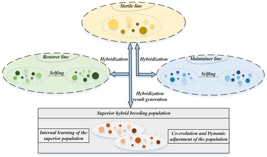
Figure 1. The principle of HBO.

(i) Hybridization Operation: This phase regenerates the sterile line through crossover between randomly selected maintainer and sterile line individuals, as formulated in Equation (1).

$$X_{\mathrm{new}}={\displaystyle \frac{r_1·X_{\mathrm{sr}}+r_2·X_{\mathrm{mr}}}{r_1+r_2}}$$

(1)

where $X_{\mathrm{mr}}$ and $X_{\mathrm{sr}}$ denote randomly sampled individuals from maintainer and sterile populations, respectively, while $r_1$ and $r_2$ ($r_1$, $r_2$∈$[-1,1]$) represent uniformly distributed random coefficients.

(ii) Selfing Operation: Restorer line individuals undergo self-evolution toward the global optimum via the self-crossing mechanism in Equation (2).

$$X_{\mathrm{new}}=r_3\left(X_{\mathrm{best}}-X_j\right)+X_i$$

(2)

where $X_{\mathrm{new}}$ is the offspring individual, $X_i$ indicates the current restorer line individual, $X_j$ is a distinct randomly selected restorer individual and satisfies the condition $i\ne j$, $X_{\mathrm{best}}$ signifies the current global optimal solution, $r_3$ is a uniform random number with values in the range $[0,1]$.

(iii) Renewal Operation: This process updates the genetic information of restorer line individuals and resets their self-crossing counters according to Equation (3).

$$X_{\mathrm{new}}=X_i+r_4\left(R_{\max }-R_{\min }\right)+R_{\min }$$

(3)

where $R_{\max }$ and $R_{\min }$ define the feasible boundary for the k-th dimension, and $r_4$ is a random variable uniformly distributed in [0, 1].

2.3. Symmetric Uncertainty

Mutual information (MI) [43] quantifies the statistical dependence between random variables. Unlike traditional correlation measures, MI accommodates both discrete and continuous variables, demonstrating a broader applicability. This measure is particularly valuable for FS due to its capacity to capture nonlinear feature relationships. The formal definition of MI is provided in Equation (4).

$$I(X,Y)=\sum _{y\in Y}\sum _{x\in X}p(x,y)log\left({\displaystyle \frac{p(x,y)}{p\left(x\right)p\left(y\right)}}\right)$$

(4)

where X and Y denote any two random variables, with $p(x,y)$ representing their joint probability distribution and $p\left(x\right)$, $p\left(y\right)$ corresponding to their marginal distributions. However, MI’s sensitivity to variable dimensionality poses limitations. To address this, symmetric uncertainty (SU) [44] introduces a normalized version of MI as shown in Equation (5).

$$U(X,Y)=2·{\displaystyle \frac{I(X,Y)}{H\left(X\right)+H\left(Y\right)}}$$

(5)

where $H\left(X\right)=-{\sum }_{x\in X}p\left(x\right)logp\left(x\right)$ is the entropy of X.

3. Proposed Approach

This section first presents the workflow of DS-IHBO, followed by a detailed explanation of the individual modules that comprise DS-IHBO.

3.1. The Workflow of DS-IHBO

The DS-IHBO FS algorithm consists of three interconnected modules: First, Module I eliminates irrelevant features to form a streamlined feature subset. Second, taking the feature subset derived from Module I as the foundational search space, Module II (the improved HBO algorithm) performs evolutionary search. During this process, Module II and Module III (the dynamic surrogate-assisted mechanism) function in parallel synergy: Module III initially constructs multiple distinct surrogate units, and subsequently dynamically selects the most appropriate surrogate unit in real time during iterations to evaluate individual updates within Module II. After a specified number of iterations, Module II switches to evaluating all individuals using the original dataset. This process continues until the iteration terminates, ultimately outputting the feature subset corresponding to the globally optimal individual. Figure 2 shows its basic workflow.

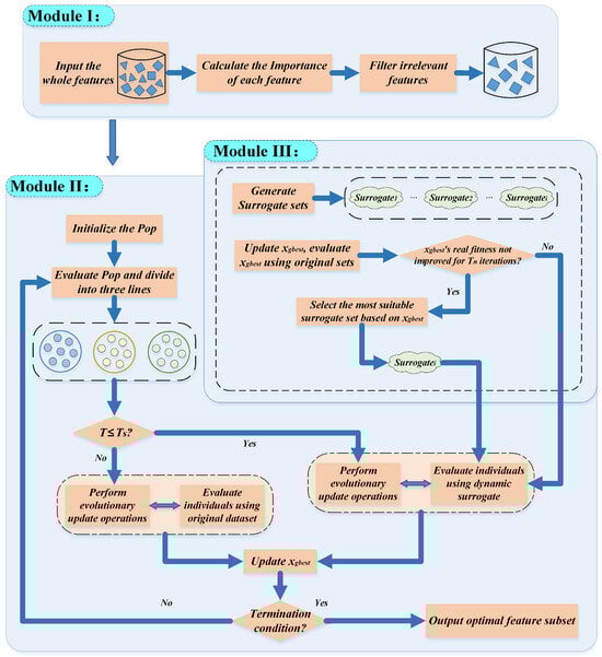
Figure 2. The workflow of DS-IHBO.

3.2. Module I: Removing Irrelevant Features

Building upon the SU measure, the interdependence $U_{ij}$ between features $F_i$ and $F_j$ can be quantified using Equation (5). However, solely considering feature–class relationships may overlook inter-feature redundancies. Inspired by max-relevance and min-redundancy (mRMR) [45], a relevance-redundancy index (${\psi }_i$) is proposed to assess feature importance. The computation involves: (1) selecting the target feature $F_i$; (2) establishing the remaining feature subset L; and (3) calculating ${\psi }_i$ for $F_i$ via Equation (6).

$${\psi }_i=U(x_i,c)-{\displaystyle \frac{1}{m-1}}\sum _{x_i\in L}U(x_i,x_j)$$

(6)

where $m-1$ denotes the number of features in L. This produces a vector encoding each feature’s class-relevance while incorporating redundancy considerations. The min-max normalization is used to normalize the relevance-redundancy index to $[0,1]$, as shown in Equation (7).

$${\psi }_i^{\ast }={\displaystyle \frac{{\psi }_i-min\left(\mathrm{\Psi }\right)}{max\left(\mathrm{\Psi }\right)-min\left(\mathrm{\Psi }\right)}},\mathrm{\Psi }=\{{\psi }_1,{\psi }_2,\dots ,{\psi }_m\}.$$

(7)

For a dataset S with D features $F=\{f_1,f_2,\dots ,f_D\}$, the value ${\psi }_i^{\ast }$ for each feature $f_i$ (where $i=1,2,\dots ,D$) is first calculated. Features with normalized relevance-redundancy indices ${\psi }_i^{\ast }$ above the specified threshold ${\rho }_0$ are identified as strongly relevant features and aggregated into a subset $F^{\prime }$. The threshold ${\rho }_0$ is crucial in determining these strongly relevance features. Traditionally, ${\rho }_0$ is set to a very small constant. However, in some datasets, all feature relevance values are relatively high. Taking the Yale_64 dataset as an instance, where typical relevance values approximate 0.5, the threshold ${\rho }_0$ is mathematically established following Song et al. [25] in Equation (8).

$${\rho }_0=min\left(0.1·{\psi }_{\max }^{\ast },{\psi }_{\lfloor D/logD\rfloor -\mathrm{th}}^{\ast }\right)$$

(8)

where $\lfloor ·\rfloor$ represents the rounding down function. Two constraints are designed in Equation (8) to balance “avoiding missing effective features” and “removing irrelevant features”:

Constraint 1: ${\psi }_{\max }^{\ast }$ is the maximum value of the normalized relevance-redundancy index (ranging from 0 to 1) in the dataset. Multiplying by 0.1 ensures that ${\rho }_0$ does not exceed 10% of the most relevant feature’s index. This avoids setting an excessively high threshold (e.g., in datasets where most ${\psi }_i^{\ast }$ are low, a fixed threshold like 0.2 might filter out all valid features). For example, if ${\psi }_{\max }^{\ast }=0.5$, this term limits ${\rho }_0$ to at most 0.05, preventing over-filtering.

Constraint 2: $\lfloor D/logD\rfloor$ represents the “recommended number of candidate features” derived from the dataset dimension D (a common empirical rule in high-dimensional FS to balance computational efficiency and information retention). ${\psi }_{\lfloor D/logD\rfloor -\mathrm{th}}^{\ast }$ is the ${\psi }_i^{\ast }$ value of the feature ranked at this “recommended number” (sorted in descending order of ${\psi }_i^{\ast }$). This constraint ensures that ${\rho }_0$ is aligned with the dataset’s dimension, avoiding excessively low thresholds (e.g., in high-dimensional datasets with $D=1000$, $\lfloor 1000/log1000\rfloor \approx 144$, so ${\rho }_0$ is at least the ${\psi }_i^{\ast }$ of the 144th feature, preventing retaining too many redundant features).

By taking the minimum of the two constraints, ${\rho }_0$ automatically adapts to the dataset’s relevance level and dimension, ensuring it is neither too high (missing valid features) nor too low (retaining noise).

3.3. Module II: The Improved HBO Algorithm

The steps of the IHBO algorithm are as follows:

(i) Population initialization with asymmetric feature stratification: Traditional random initialization often exhibits strong distributional symmetry, leading to populations concentrated in limited regions of the search space and consequently reducing population diversity. To break this symmetry and introduce controlled asymmetry, a novel initialization mechanism based on the relevance-redundancy index is proposed, as detailed in Algorithm 1.

Specifically, features are first divided into three groups reflecting asymmetric relevance levels: the top 10% as high-relevance, the next 10–50% as mid-relevance, and the remaining 50% as low-relevance. This stratified division intentionally introduces structural asymmetry to prioritize features with high discriminative power. For each individual, the number of features to be initialized, denoted by $\mu$, is randomly drawn from the interval $[0,0.3D]$, where D is the total feature dimension. All high-relevance features are symmetrically included to ensure essential information retention, while mid- and low-relevance features are asymmetrically sampled: $\theta ·\mu$ features from the mid-relevance group and $(1-\theta )·\mu$ from the low-relevance group, where $\theta$ follows a uniform distribution over $[0.7,1]$. This asymmetric sampling strategy effectively balances diversity and relevance, reduces redundancy, and promotes symmetric compactness within the selected feature subsets. The process repeats until a population of size $NP$ is constructed.

Algorithm 1 Population initialization strategy

1: Input: $NP$: population size; D: feature dimension   2: Output: P: initial population   3: for  $i=1,2,\dots ,D$ do   4:    Calculate relevance-redundancy index (i)   5: end for   6: Sort features according index (i)   7: High-relevance in the top 10%; mid-relevance in the top 10–50%; low-relevance in the bottom 50%   8: for $n=1,2,\dots ,NP$ do   9:    $\mu \leftarrow$ Randomly generate in $[0,0.3·D]$ 10:    Select all high-relevance features 11:    $\theta \leftarrow$ Randomly generate in $[0.7,1]$ 12:    Randomly select $\theta ·\mu$ mid-relevance features and $(1-\theta )·\mu$ low-relevance features 13:    for $i=1,2,\dots ,D$ do 14:      if i is selected then 15:         $F\left(i\right)=1$ 16:      end if 17:    end for 18: end for 19: return initial population P

(ii) An update strategy for the maintainer line: In HBO, the maintainer line represents a group of individuals with optimal fitness values. It is used to cross with the sterile line to generate improved sterile individuals with superior traits, thereby guiding the direction of population updates. However, the original HBO does not establish an effective strategy for updating the maintainer line. To address this limitation, this paper proposes an improvement to the maintainer line’s update based on a dynamic selection strategy of adaptive differential operators. Given that differential operators have multiple variants, and each is tailored to distinct types of search tasks, the objective is to integrate the advantages of these diverse differential variants. Accordingly, three improved differential operator variants are proposed: a global differential operator for the global search phase, a transitional one for the transition from global to local search, and a local one for the local search phase. These three differential operators are denoted as $D{E}_1$, $D{E}_2$, and $D{E}_3$, respectively, as shown in Equations (9)–(11).

$$D{E}_1:x_i^j\left(t\right)+r_1·\left(x_{p_1}^j\left(t\right)-x_{p_2}^j\left(t\right)\right)+(1-r_1)·\left(x_{p_3}^j\left(t\right)-x_i^j\left(t\right)\right)$$

(9)

where $r_1$ and $r_2$ are random values in the range of 0 to 1, $p_m$ represents randomly selected individuals from the population. They satisfy conditions $(p_m\ne i)$ and $(p_i\ne p_j, i\ne j,$ $1\le i, j\le 4)$. The term $r_1·(x_{p_1}^j\left(t\right)-x_{p_2}^j\left(t\right))$ creates a perturbation vector based on the difference between two randomly chosen individuals. This encourages the search to span wide areas of the solution space. The second term, $(1-r_1)·(x_{p_3}^j\left(t\right)-x_i^j\left(t\right))$, adds another layer of random perturbation relative to the current individual’s position, further enhancing diversity and preventing premature convergence. The strength of this operator lies in its ability to discover new and potentially promising regions, which is critical in the early stages.

$$D{E}_2:x_i^j\left(t\right)+F·\left(x_{p_1}^j\left(t\right)-x_{p_2}^j\left(t\right)\right)+F·\left(x_{\mathrm{best}}^j\left(t\right)-x_i^j\left(t\right)\right)$$

(10)

where $x_{\mathrm{best}}^j\left(t\right)$ represents the value of the j-th dimension of the best solution in the current generation. $D{E}_2$ incorporates both a random perturbation term ($x_{p_1}^j\left(t\right)-x_{p_2}^j\left(t\right)$) for exploration and a term that guides the search toward the best solution ($x_{\mathrm{best}}^j\left(t\right)-x_i^j\left(t\right)$) for exploitation. It provides a smooth transition from a global, explorative search to a local, exploitative one.

$$D{E}_3:x_{\mathrm{best}}^j\left(t\right)+r_2·\left(x_{p_1}^j\left(t\right)-x_{p_2}^j\left(t\right)\right)+(1-r_2)·\left(x_{p_3}^j\left(t\right)-x_{p_4}^j\left(t\right)\right)$$

(11)

where F is the scaling factor that controls the transition of the population from global search to local search. The search is anchored to $x_{\mathrm{best}}^j\left(t\right)$, the best solution found so far. The subsequent perturbation terms are relatively small variations created from the differences in random individuals. This structure ensures that the search is concentrated in the promising region around the current best solution, allowing for fine-tuning and convergence towards a refined optimum. This is essential in the later stages of the algorithm.

To enable the algorithm to use different selection probabilities for differential strategies in different optimization stages, the probability selection strategies are defined as follows. In the early stage of optimization, a higher probability is assigned to the exploratory strategy $D{E}_1$. In the middle stage, the probability gradually shifts to the balancing strategy $D{E}_2$. In the later stage of optimization, a higher probability is assigned to the exploitative strategy $D{E}_3$ to refine the solutions. This paper introduces an adaptive probability generation mechanism to dynamically produce the selection probabilities of the three differential strategies, using the roulette_wheel_selection $\left(p_i\right)$ algorithm to determine $D{E}_i$. As shown in Equations (12)–(17).

$$s_1={\displaystyle \frac{peak}{1+exp\left(-\frac{(t-T/6)}{T/25}\right)}}+s_{min}$$

(12)

$$s_2=peak·exp\left(-{\displaystyle \frac{{(t-T/2)}^2}{10·T}}\right)+s_{min}$$

(13)

$$s_3={\displaystyle \frac{peak}{1+exp\left(-\frac{(t-5·T/6)}{T/25}\right)}}+s_{min}$$

(14)

$$peak=s_{max}-s_{min}$$

(15)

$$S=s_1+s_2+s_3$$

(16)

$$p_i={\displaystyle \frac{s_i}{S}},i=1,2,3$$

(17)

where $s_{min}$ and $s_{max}$ are boundary correction parameters to prevent values before normalization from being too small or too large. $p_i(i=1,2,3)$ represents the normalized probability that the i-th difference operator is selected, t and T represent the current iteration number and the maximum iteration number, respectively. Figure 3 demonstrates the trend of adaptive adjustment for the selection probabilities of the three differential strategies as the number of iterations increases.

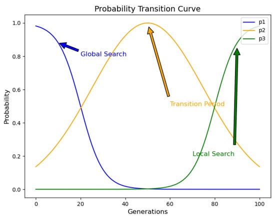
Figure 3. The probability transfer curve of differential operators.

As shown in Figure 3, in the early stage of evolution, the algorithm focuses on exploring the global search space to find more promising regions. Therefore, the probability of selecting the global exploration strategy $D{E}_1$ is higher. As evolution progresses, the optimization process gradually transitions from global search to local search. To smoothly transition between these two stages, the algorithm gradually decreases the probability of selecting the global exploration strategy $D{E}_1$ and increases the probability of selecting the balancing strategy $D{E}_2$. In the later stage of evolution, the selection gradually shifts to the local exploitation strategy $D{E}_3$ to enhance the search in the vicinity of the optimal solution.

(iii) Modifications to the hybridization and selfing phases: The objective of the hybridization phase is to update the sterile line. However, the original update strategy does not fully consider the difference between the exploration phase in the early stage and the exploitation phase in the later stage. Therefore, this paper introduces a t-distribution mutation disturbance strategy to improve the hybridization phase. The t-distribution, also known as the Student’s t-distribution, is characterized by its degree of freedom ($df$) and mutation scale ($\sigma$). The degree of freedom controls the shape of the distribution, mainly affecting the thickness of the tails, while $\sigma$ determines the width of the distribution. Based on the characteristics of t-distribution, this paper improves the hybridization phase as shown in Equations (18)–(21).

$$X_{\mathrm{new}\left(i\right)}^d\left(t\right)=t·X_s^d\left(t\right)+(1-t)·X_m^d\left(t\right)$$

(18)

$$f(t\mid df,\sigma )={\displaystyle \frac{\mathrm{\Gamma }\left(\frac{df+1}{2}\right)}{\mathrm{\Gamma }\left(\frac{df}{2}\right)\sqrt{df\pi \sigma }}}{\left(1+{\displaystyle \frac{1}{df}}{\left({\displaystyle \frac{t}{\sigma }}\right)}^2\right)}^{-{\displaystyle \frac{df+1}{2}}}$$

(19)

$$df=2+{\displaystyle \frac{t}{T}}·28$$

(20)

$$\sigma =({\sigma }_{max}-{\sigma }_{min})·\left(1-{\left({\displaystyle \frac{t}{T}}\right)}^{gr}\right)+{\sigma }_{min}$$

(21)

The random number r of the original hybridization stage is replaced by random sampling of t-distribution. $X_{\mathrm{new}\left(i\right)}^d\left(t\right)$ represents a new sterile individual generated by hybridization, where each dimension is disturbed by the random variables generated by t-distribution. $\Gamma$ represents the Gamma function. ${\sigma }_{max}$ and ${\sigma }_{min}$ denote the maximum and minimum values of the mutation scale, which control the range of generated random numbers. The larger the mutation scale, the larger the range of generated random numbers, and vice versa. $gr$ is the growth rate, which controls the curvature of the $\sigma$ change curve.

Figure 4 shows the changes in the shape of the t-distribution under different degrees of freedom and mutation scales. When the degree of freedom is one, the t-distribution becomes a Cauchy distribution with heavy tails. As the degree of freedom increases, the heavy tails lessen, gradually approaching a normal distribution. A larger mutation scale results in a wider t-distribution curve, indicating more dispersed data points, while a smaller mutation scale narrows the distribution, concentrating the data points. Therefore, this paper leverages the characteristics of the t-distribution by combining different degrees of freedom and mutation scales to control its shape, thereby managing the global and local update strategies of individuals. Specifically, in the initial iteration stages, smaller degrees of freedom and larger mutation scales make the t-distribution similar to the Cauchy distribution with dispersed data, generating larger perturbations that favor global search. As iterations progress, increasing degrees of freedom and decreasing mutation scales cause the t-distribution to approach a standard normal distribution with smaller variance, resulting in smaller perturbations and a preference for local search.

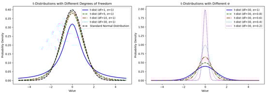
Figure 4. The shape of t-distribution corresponding to different degrees of freedom and mutation scales.

The selfing phase focuses on updating the restorer line. When a restorer individual reaches the maximum number of selfings, it is considered to have fallen into a local optimum. At this point, the renewal operation is triggered for the individual, which plays a decisive role in the transition between selfing and renewal. Instead of setting a constant value in the original HBO algorithm, this paper introduces an enhanced selfing upper bound, as defined in Equation (22).

$$SC=S{C}_{\min }+\left(S{C}_{\max }-S{C}_{\min }\right)·\left(1-{\left({\displaystyle \frac{t}{T}}\right)}^2\right)$$

(22)

where $S{C}_{\min }$ and $S{C}_{\max }$ represent the minimum and maximum bounds for selfing count, respectively. In the early iterations, the algorithm is in the global search phase, and most individuals could perform effective updates within a few cycles. Therefore, $SC$ is set to a large value. If an individual reaches this bound early, it indicates that it has fallen into a local optimum, which will trigger the renewal operation. As optimization progresses to later iterations, the possibility of an individual falling into a local optimum increases. Therefore, setting $SC$ to a smaller value in later stages helps an individual escape the local optimum more quickly.

Collectively, these three improvements are specifically designed to address the core challenges of high-dimensional FS. The asymmetric population initialization addresses the massive search space and feature redundancy: a relevance-redundancy index guides initial searches toward promising feature combinations, effectively pruning unpromising directions from the outset. The adaptive update strategy for the maintainer line delivers the required dynamic balance between exploration and exploitation. Broad exploration in the early stage is critical for navigating the vast feature space, while focused exploitation in the later stage refines the optimal feature subset. Modifications to the hybridization and selfing phases act as mechanisms to preserve population diversity and avoid local optima. The adaptive shape of the t-distribution enables large perturbations for global exploration when required, and the dynamic selfing count ensures the renewal of stagnated individuals, preventing premature convergence.

To analyze the impact of the proposed improved strategy on algorithm time complexity, a comprehensive comparison between HBO and IHBO is conducted at each stage. With population size N, problem dimension D, and maximum iteration number T assumed, the results of the comparative analysis are shown in Table 3.

Table 3. Time complexity comparison.

Step	HBO	IHBO
Population initialization	$O\left(N\right)$	$O\left(max\right(D·logD,N·D\left)\right)$
Update of maintainer line	-	$O(N·D/3)$
Hybridization	$O(N·D/3)$	$O(N·D/3)$
Selfing	$O(N·D/3)$	$O(N·D/3)$
Sort individuals	$O\left(N\right)$	$O\left(N\right)$
Update of the optimal solution	$O\left(1\right)$	$O\left(1\right)$
The overall time-complexity	$O(T·(N+2N·D/3+1)+N)$	$O(T·(N+N·D+1)+max(D·logD,N·D\left)\right)$

Based on the analysis, IHBO’s time complexity in the population initialization stage is approximately D times that of HBO. However, since population initialization occurs only once, its impact on overall time complexity is relatively minor. In the population update stage, IHBO adds only the maintainer line update process compared with HBO, which increases time complexity by approximately 1/3 but significantly enhances the utilization rate of superior individuals and population diversity. Regarding population sorting and best solution update, both algorithms exhibit identical time complexity. Overall, IHBO marginally increases computational overhead only during population initialization and maintainer line update stages. When HBO’s population size is set to approximately 1.5 times that of IHBO, comparable total time complexity can be achieved.

3.4. Module III: Dynamic Surrogate-Assisted Mechanism

(i) Generation of surrogate units by density-adaptive symmetric sampling: To effectively handle imbalanced data distributions while maintaining representative symmetry between majority and minority classes, an adaptive K-Nearest Neighbors (KNN) algorithm is introduced. This method dynamically adjusts the number of neighbors K based on local density to discriminate between class-central and class-boundary samples. For a given sample $s_i$, the local density $D_i$ is computed as the average distance to its k nearest neighbors, as formalized in Equation (23).

$$D_i={\displaystyle \frac{1}{k}}\sum _{j=1}^{k}d(s_i,s_j)$$

(23)

Based on $D_i$, the number of neighbors $K_i$ is determined by a threshold $D_{\mathrm{threshold}}$, typically the median of all $D_i$ in Equation (24).

$$K_i=\left\{\begin{array}{cc}{K}_{\max },\hfill & \mathrm{if}{D}_i\le D_{\mathrm{threshold}}\hfill \\ K_{\min },\hfill & \mathrm{if}{D}_i>D_{\mathrm{threshold}}\hfill \end{array}\right.$$

(24)

Subsequently, the algorithm determines whether the $K_i$ nearest neighbors of a given sample belong to the same class; if so, the sample is classified as central, otherwise as boundary, as illustrated in Figure 5.

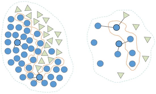
Figure 5. Boundary division based on adaptive KNN. The dashed lines represent the boundary of the class, and different colors represent different classes.

In imbalanced datasets, the average number of samples per class, denoted as $\overline{N}$, is first calculated. Classes with more than $\overline{N}$ samples are defined as majority classes, while those with $\overline{N}$ or fewer are identified as minority classes. The adaptive KNN algorithm is then applied to distinguish between central samples and boundary samples.

Since majority classes contain substantially more samples than minority ones, using all majority class samples for training would significantly increase computational cost. To mitigate redundancy, all boundary samples are retained in their entirety, as they contain critical information for classification models, while 40% of central samples are randomly sampled, given that they are typically redundant.

Although minority classes have fewer samples, they are crucial for the model. To prevent their influence from being overshadowed by majority classes, the average number of samples $N_{\mathrm{maj}}$ across all majority classes is first calculated. The SMOTE [46] oversampling technique is then applied to expand minority classes to $N_{\mathrm{maj}}$. All boundary samples are retained, and 40% of the central samples are randomly selected. Representative samples from both majority and minority classes are combined to form the final set of representative samples. Based on these samples, multiple surrogate units are constructed.

The total number of samples in each dataset is denoted as N. To balance accuracy and computational cost, six surrogate units with different sample sizes are constructed as follows:

Step 1.

Calculate the target sample sizes for the six surrogate units based on preset proportions of the original dataset size N: 0.75N, 0.65N, 0.55N, 0.45N, 0.35N, and 0.25N;

Step 2.

Based on the representative sample set, calculate the sample size for each category and determine the proportion of each category: category sample size/total sample size. Set this as the target category proportion to ensure that subsequent surrogate unit construction selects samples from each category according to the same proportion;

Step 3.

Apply agglomerative clustering algorithm to partition the representative sample set into six clusters;

Step 4.

Each surrogate unit selects a certain number of target samples evenly from the six clusters. For example, in the first surrogate unit, the algorithm needs to select 0.75N/6 samples from each cluster;

Step 5.

Traverse the six clusters. Within each cluster, select samples for each category based on the required number of category samples (target category proportion × target sample number from the previous step). If the cluster contains no samples of a particular category, skip that category. If the number of samples for a certain category within the cluster is less than or equal to the required category sample number, select all samples; otherwise, calculate the centroid of that category’s samples in the current cluster and prioritize selecting the required number of samples that are farthest from the centroid (i.e., most representative);

Step 6.

After completing sample selection for each cluster, check whether the proportion of each category in the surrogate unit conforms to the target category proportion. For categories that do not conform, perform global random supplementation from the remaining unselected samples until reaching the target category proportion (i.e., achieving the target sample number for each surrogate unit).

(ii) Dynamic symmetry-preserving surrogate assistance: The surrogate unit selection process begins with population initialization, where the original dataset S serves as the evaluation benchmark. The global optimal individual $x_{gbest}$, possessing the optimal ground truth fitness $f_0$, is first identified. Subsequently, l surrogate units generate corresponding fitness values $\{f_1,f_2,\dots ,f_l\}$ for $x_{gbest}$. By comparing the prediction errors $|f_i-f_0|$, the most accurate surrogate unit (with minimal deviation) is selected for feature subset evaluation in subsequent iterations.

During the initial $T_s$ iterations, the feature subsets are evaluated using the surrogate unit, which is periodically updated to ensure alignment with the true dataset distribution. However, overly frequent updates may impair the population’s ability to adapt to evolving search environments. Consequently, the surrogate unit is only refreshed when the global optimum individual $x_{gbest}^t$ shows no improvement in its real fitness after $T_n$ consecutive iterations. The surrogate selection mechanism follows the initialization approach described above, with the current $x_{gbest}^t$ replacing the previous $x_{gbest}$ as the reference solution. Upon completing the surrogate phase (i.e., after $T_s$ iterations), candidate solutions are evaluated against the original dataset. Our investigation of six $T_s$ values (0, 25, 50, 75, and 100) revealed 75 as the optimal setting. The complete dynamic surrogate-assisted IHBO method is summarized in Algorithm 2.

Algorithm 2 Dynamic surrogate combining with IHBO

1: Input: Surrogate units: $S_1,S_2,S_3,S_4,S_5,S_6$.   2: Output: A feature subset.   3: Initialize IHBO Population, find $x_{gbest}$ using the original dataset.   4: Select the most appropriate surrogate unit based on $x_{gbest}$.   5: while$T_{max}$ is not reached do   6:    if $T\le T_s$ then   7:      Maintainer-update();   8:      Hybridization();   9:      Selfing(); 10:      Evaluate individuals using surrogate unit; 11:      Update $x_{gbest}$, evaluate $x_{gbest}$ using original dataset. 12:      if $x_{gbest}$’s real fitness is not improved for $T_u$ iterations then 13:         Select the most appropriate surrogate unit based on $x_{gbest}$. 14:      end if 15:    else 16:      Maintainer-update(); 17:      Hybridization(); 18:      Selfing(); 19:      Evaluate individuals using original dataset; 20:      Update $x_{gbest}$. 21:    end if 22:    $T=T+1$ 23: end while 24: return $x_{gbest}$ as the final feature subset.

The computational complexity of the proposed algorithm mainly includes the following aspects: (1) The complexity of filtering out irrelevant features in Module I is $O(D·S)$; (2) Module II and Module III are executed in parallel. The complexity of implementing IHBO is $O(T·(N+N·D^{\prime }+1)+max(D^{\prime }·log{D}^{\prime },N·D^{\prime }))$, and thus, the complexity after adopting the dynamic surrogate mechanism is approximately $O(T_s·N·D^{\prime }+(T-T_s)·N·S·D^{\prime })$. In the above process, D denotes the number of features in the original data, S denotes the number of samples in the original data, $D^{\prime }$ denotes the number of reduced features after the first stage, T denotes the number of iterations, $T_s$ denotes the number of surrogate iterations, and N denotes the population size.

4. Experiments

This section first presents ablation experiments on Module I and Module III to verify the effectiveness of their core designs. Second, it introduces the fitness function and datasets, and details five state-of-the-art comparative methods along with their parameter configurations. It then presents comprehensive experimental comparisons between DS-IHBO and the five FS methods on 12 publicly available datasets, using five evaluation metrics. Finally, it includes sensitivity analysis on the key parameters of DS-IHBO in the surrogate phase, including ablation verification of Module III.

4.1. Datasets

To demonstrate the advantages of the proposed algorithm, comprehensive comparisons are conducted with six established methods across 12 datasets—all of which are open-source and sourced from http://archive.ics.uci.edu/ml (accessed on 4 September 2025), https://jundongl.github.io/scikit-feature/datasets.html (accessed on 4 September 2025) and https://ckzixf.github.io/dataset.html (accessed on 4 September 2025). These datasets encompass key domains, including medical diagnosis (DLBCL, Parkinson, GLIOMA, Lung2, BrainTumor1, Lymphoma, 11_Tumor), bioinformatics (Musk2), computer vision (USPS), text mining (RELATHE), and industrial and Web (PCMAC, InternetAd). The datasets highlight the following characteristics: (1) inclusion of both binary classification and multi-classification; (2) large sample sizes: The USPS dataset contains the highest number of samples, with a total of 9298 instances; (3) high-dimensionality: The 11_Tumor dataset includes 12,533 features; (4) class imbalance: all datasets are imbalanced, with the Lung2 dataset exhibiting the most significant imbalance ratio of 4.32%. Table 4 presents the essential information of the datasets used in this study, where Max indicates the number of majority class samples, Min indicates the number of minority class samples, and the imbalance rate indicates the ratio of Min to Max.

Table 4. Essential information of the 12 datasets.

Dataset	Feature	Sample	Class	Max	Min	Imbalance Ratio (%)
DLBCL	5469	77	2	58	19	32.76
PCMAC	3289	1943	2	982	961	97.86
Musk2	166	6598	2	5581	1017	18.22
RELATHE	4322	1427	2	779	648	83.18
Parkinson	754	756	2	564	192	34.04
InternetAd	1558	3279	2	2820	459	16.28
GLIOMA	4434	50	4	15	7	50.00
Lung2	3312	203	5	139	6	4.32
BrainTumor1	5920	90	5	60	4	6.67
Lymphoma	4026	96	9	46	2	4.35
USPS	256	9298	10	1553	708	45.59
11_Tumor	12,533	174	11	27	6	22.22

To ensure the quality and consistency of experimental data, data preprocessing is performed for each dataset. This process included the following steps: missing values are imputed using the mean of the corresponding feature columns; categorical features are converted to integer format via one-hot encoding; and all feature values are scaled to a unified standard range using min-max normalization.

4.2. Ablation Experiments for Module I

This section analyzes the algorithm without the filter module (denoted as DS-IHBO/Module I). The accuracy (Acc) and running time of this algorithm are compared with those of the proposed DS-IHBO in Table 5. On the high-dimensional USPS dataset, DS-IHBO dynamically adapts threshold ${\rho }_0$ to eliminate redundant features while retaining classification-critical core features in the filtering stage. This slightly improves accuracy from 96.21% to 96.57% and reduces running time to 6872.09 s (a decrease of approximately 34%), further validating the filtering stage’s necessity. In contrast, DS-IHBO/Module I exhibits limitations. Redundant noise in full features interferes with classifier decisions, leading to consistently lower Acc than DS-IHBO. Additionally, the high-dimensional space increases IHBO’s evolutionary burden: more feature combinations require fitness evaluation per iteration, and the search tends to fall into redundant-feature-dominated local optima, ultimately reducing efficiency.

Table 5. Acc and running time (unit: s) obtained by DS-IHBO/Module I and DS-IHBO.

Datasets	DS-IHBO/Module I			DS-IHBO
	Acc(std)	Time		Acc(std)	Time
DLBCL	100.00(0.00)	106.47		100.00(0.00)	20.58
PCMAC	90.64(0.89)	3043.26		91.18(0.56)	2326.07
Musk2	95.37(0.73)	4718.34		95.91(0.39)	3443.67
RELATHE	90.85(0.68)	1982.15		91.30(0.44)	625.06
Parkinson	94.26(1.04)	518.73		94.91(0.67)	145.90
InternetAd	96.38(0.51)	2924.68		96.95(0.28)	882.81
GLIOMA	91.37(0.97)	57.42		92.20(0.65)	29.77
Lung2	98.29(0.48)	108.15		98.62(0.25)	34.87
BrainTumor1	92.15(1.58)	112.13		92.58(1.25)	26.64
Lymphoma	96.02(0.73)	107.65		96.49(0.41)	23.54
USPS	96.21(0.87)	10,436.88		96.57(0.53)	6872.09
11_Tumor	91.28(1.82)	385.47		91.65(1.47)	48.37

4.3. Ablation Experiments for Module II

The IHBO algorithm integrates four key strategies: stratified population initialization (HBO_IN), adaptive difference operator-based maintainer line update (HBO_MA), t-distribution-driven mutation for hybridization (HBO_HY), and enhanced selfing upper bound for selfing phase (HBO_SE). Each addresses specific algorithmic weaknesses, and their combination aims to boost overall performance.

For fair comparison and to validate the effectiveness of each strategy, 30 independent runs of each algorithm are performed on every test function (across dimensions) to reduce the impact of randomness. Maximum iterations are uniformly set to 1000. For consistent fitness evaluations, IHBO and HBO_MA used a population size of 40, while the original HBO and the other three variants used 60. Performance is evaluated using five metrics: best/worst/average fitness (best, worst, avg), standard deviation (std), and average runtime (time). Table 6, Table 7, Table 8 and Table 9 present the results for all algorithms on CEC2022 benchmarks (10D and 20D, respectively).

Table 6. Performance comparison of IHBO and other variants on CEC2022 (Dim = 10) (F1–F6).

Func	Metric	HBO	HBO_IN	HBO_MA	HBO_HY	HBO_SE	IHBO
F1	Best	$3.00\times {10}^2$	$3.00\times {10}^2$	$3.00\times {10}^2$	$3.00\times {10}^2$	$3.00\times {10}^2$	$3.00\times {10}^2$
	Worst	$3.01\times {10}^2$	$3.00\times {10}^2$	$3.40\times {10}^2$	$3.00\times {10}^2$	$3.01\times {10}^2$	$3.00\times {10}^2$
	Mean	$3.00\times {10}^2$	$3.00\times {10}^2$	$3.02\times {10}^2$	$3.00\times {10}^2$	$3.00\times {10}^2$	$3.00\times {10}^2$
	Std	$1.09\times {10}^{-1}$	$8.14\times {10}^{-2}$	$7.77\times {10}^0$	$1.66\times {10}^{-3}$	$1.04\times {10}^{-1}$	$\mathbf{1.32}\times {\mathbf{10}}^{-\mathbf{13}}$
	Time (s)	1.09	1.09	1.15	0.99	1.08	1.21
F2	Best	$4.00\times {10}^2$	$4.00\times {10}^2$	$4.00\times {10}^2$	$4.04\times {10}^2$	$4.00\times {10}^2$	$4.00\times {10}^2$
	Worst	$4.53\times {10}^2$	$4.65\times {10}^2$	$4.12\times {10}^2$	$4.11\times {10}^2$	$4.71\times {10}^2$	$\mathbf{4.09}\times {\mathbf{10}}^{\mathbf{2}}$
	Mean	$4.03\times {10}^2$	$4.03\times {10}^2$	$4.03\times {10}^2$	$4.07\times {10}^2$	$4.06\times {10}^2$	$4.05\times {10}^2$
	Std	$9.61\times {10}^0$	$1.17\times {10}^1$	$4.07\times {10}^0$	$\mathbf{2.23}\times {\mathbf{10}}^{\mathbf{0}}$	$1.85\times {10}^1$	$3.20\times {10}^0$
	Time (s)	1.26	1.26	1.31	1.12	1.21	1.36
F3	Best	$6.00\times {10}^2$	$6.00\times {10}^2$	$6.00\times {10}^2$	$6.00\times {10}^2$	$6.00\times {10}^2$	$6.00\times {10}^2$
	Worst	$6.00\times {10}^2$	$6.00\times {10}^2$	$6.00\times {10}^2$	$6.00\times {10}^2$	$6.00\times {10}^2$	$6.00\times {10}^2$
	Mean	$6.00\times {10}^2$	$6.00\times {10}^2$	$6.00\times {10}^2$	$6.00\times {10}^2$	$6.00\times {10}^2$	$6.00\times {10}^2$
	Std	$1.21\times {10}^{-3}$	$1.13\times {10}^{-7}$	$1.25\times {10}^{-4}$	$1.32\times {10}^{-11}$	$1.82\times {10}^{-8}$	$\mathbf{7.48}\times {\mathbf{10}}^{-\mathbf{14}}$
	Time (s)	1.57	1.57	1.63	1.54	1.65	1.74
F4	Best	$8.08\times {10}^2$	$8.14\times {10}^2$	$8.08\times {10}^2$	$8.30\times {10}^2$	$8.08\times {10}^2$	$8.14\times {10}^2$
	Worst	$8.31\times {10}^2$	$8.31\times {10}^2$	$8.30\times {10}^2$	$8.69\times {10}^2$	$\mathbf{8.22}\times {\mathbf{10}}^{\mathbf{2}}$	$8.55\times {10}^2$
	Mean	$8.20\times {10}^2$	$8.20\times {10}^2$	$8.18\times {10}^2$	$8.51\times {10}^2$	$\mathbf{8.15}\times {\mathbf{10}}^{\mathbf{2}}$	$8.30\times {10}^2$
	Std	$5.20\times {10}^0$	$4.25\times {10}^0$	$4.96\times {10}^0$	$1.11\times {10}^1$	$\mathbf{4.06}\times {\mathbf{10}}^{\mathbf{0}}$	$8.89\times {10}^0$
	Time (s)	1.97	1.96	2.02	2.03	2.29	2.26
F5	Best	$9.00\times {10}^2$	$9.00\times {10}^2$	$9.00\times {10}^2$	$9.00\times {10}^2$	$9.00\times {10}^2$	$9.00\times {10}^2$
	Worst	$9.00\times {10}^2$	$9.00\times {10}^2$	$9.00\times {10}^2$	$9.00\times {10}^2$	$9.00\times {10}^2$	$9.00\times {10}^2$
	Mean	$9.00\times {10}^2$	$9.00\times {10}^2$	$9.00\times {10}^2$	$9.00\times {10}^2$	$9.00\times {10}^2$	$9.00\times {10}^2$
	Std	$1.14\times {10}^{-1}$	$1.74\times {10}^{-4}$	$8.29\times {10}^{-2}$	$4.85\times {10}^{-7}$	$1.14\times {10}^{-1}$	$\mathbf{0.00}\times {\mathbf{10}}^{\mathbf{0}}$
	Time (s)	1.45	1.44	1.49	1.28	1.39	1.56
F6	Best	$3.67\times {10}^3$	$5.22\times {10}^3$	$\mathbf{1.81}\times {\mathbf{10}}^{\mathbf{3}}$	$1.32\times {10}^4$	$2.16\times {10}^3$	$1.84\times {10}^3$
	Worst	$1.47\times {10}^4$	$2.80\times {10}^4$	$\mathbf{2.24}\times {\mathbf{10}}^{\mathbf{3}}$	$5.15\times {10}^4$	$9.63\times {10}^3$	$3.88\times {10}^4$
	Mean	$9.56\times {10}^3$	$1.07\times {10}^4$	$\mathbf{1.88}\times {\mathbf{10}}^{\mathbf{3}}$	$3.34\times {10}^4$	$5.10\times {10}^3$	$8.01\times {10}^3$
	Std	$2.45\times {10}^3$	$4.82\times {10}^3$	$\mathbf{1.06}\times {\mathbf{10}}^{\mathbf{2}}$	$1.08\times {10}^4$	$1.98\times {10}^3$	$7.15\times {10}^3$
	Time (s)	1.47	1.46	1.52	1.52	1.61	1.74

Table 7. Performance comparison of IHBO and other variants on CEC2022 (Dim = 10) (F7–F12).

Func	Metric	HBO	HBO_IN	HBO_MA	HBO_HY	HBO_SE	IHBO
F7	Best	$2.02\times {10}^3$	$2.02\times {10}^3$	$2.02\times {10}^3$	$2.01\times {10}^3$	$2.02\times {10}^3$	$\mathbf{2.00}\times {\mathbf{10}}^{\mathbf{3}}$
	Worst	$2.03\times {10}^3$	$2.03\times {10}^3$	$\mathbf{2.02}\times {\mathbf{10}}^{\mathbf{3}}$	$2.08\times {10}^3$	$2.04\times {10}^3$	$2.03\times {10}^3$
	Mean	$2.02\times {10}^3$	$2.02\times {10}^3$	$2.02\times {10}^3$	$2.04\times {10}^3$	$2.03\times {10}^3$	$2.02\times {10}^3$
	Std	$1.36\times {10}^0$	$1.41\times {10}^0$	$\mathbf{1.11}\times {\mathbf{10}}^{\mathbf{0}}$	$1.65\times {10}^1$	$3.68\times {10}^0$	$5.05\times {10}^0$
	Time (s)	11.55	11.56	11.58	11.64	11.74	11.80
F8	Best	$2.20\times {10}^3$	$2.20\times {10}^3$	$2.20\times {10}^3$	$2.22\times {10}^3$	$2.23\times {10}^3$	$2.20\times {10}^3$
	Worst	$2.23\times {10}^3$	$2.23\times {10}^3$	$2.23\times {10}^3$	$2.23\times {10}^3$	$2.39\times {10}^3$	$2.23\times {10}^3$
	Mean	$2.22\times {10}^3$	$2.22\times {10}^3$	$2.22\times {10}^3$	$2.23\times {10}^3$	$2.26\times {10}^3$	$2.22\times {10}^3$
	Std	$1.03\times {10}^1$	$1.02\times {10}^1$	$9.89\times {10}^0$	$\mathbf{2.23}\times {\mathbf{10}}^{\mathbf{0}}$	$3.12\times {10}^1$	$9.65\times {10}^0$
	Time (s)	15.73	15.69	15.78	15.83	15.89	16.44
F9	Best	$2.30\times {10}^3$	$2.30\times {10}^3$	$2.30\times {10}^3$	$2.30\times {10}^3$	$2.67\times {10}^3$	$2.30\times {10}^3$
	Worst	$2.66\times {10}^3$	$2.67\times {10}^3$	$2.75\times {10}^3$	$2.66\times {10}^3$	$2.75\times {10}^3$	$2.67\times {10}^3$
	Mean	$2.52\times {10}^3$	$2.47\times {10}^3$	$2.50\times {10}^3$	$2.54\times {10}^3$	$2.70\times {10}^3$	$\mathbf{2.43}\times {\mathbf{10}}^{\mathbf{3}}$
	Std	$1.76\times {10}^2$	$1.79\times {10}^2$	$1.83\times {10}^2$	$1.69\times {10}^2$	$\mathbf{2.20}\times {\mathbf{10}}^{\mathbf{1}}$	$1.74\times {10}^2$
	Time (s)	3.38	3.38	3.44	3.26	3.30	3.51
F10	Best	$2.47\times {10}^3$	$2.62\times {10}^3$	$2.73\times {10}^3$	$2.59\times {10}^3$	$\mathbf{2.77}\times {\mathbf{10}}^{\mathbf{3}}$	$2.74\times {10}^3$
	Worst	$-1.18\times {10}^3$	$1.02\times {10}^3$	$9.13\times {10}^2$	$-1.09\times {10}^3$	$\mathbf{2.30}\times {\mathbf{10}}^{\mathbf{3}}$	$3.93\times {10}^2$
	Mean	$1.06\times {10}^3$	$2.35\times {10}^3$	$2.39\times {10}^3$	$9.33\times {10}^2$	$\mathbf{2.68}\times {\mathbf{10}}^{\mathbf{3}}$	$2.30\times {10}^3$
	Std	$7.31\times {10}^2$	$4.15\times {10}^2$	$4.58\times {10}^2$	$9.95\times {10}^2$	$\mathbf{1.14}\times {\mathbf{10}}^{\mathbf{2}}$	$6.36\times {10}^2$
	Time (s)	3.33	3.32	3.38	3.19	3.30	3.45
F11	Best	$2.60\times {10}^3$	$2.60\times {10}^3$	$2.60\times {10}^3$	$2.60\times {10}^3$	$2.60\times {10}^3$	$2.60\times {10}^3$
	Worst	$2.62\times {10}^3$	$2.60\times {10}^3$	$2.60\times {10}^3$	$3.46\times {10}^3$	$2.60\times {10}^3$	$2.60\times {10}^3$
	Mean	$2.60\times {10}^3$	$2.60\times {10}^3$	$2.60\times {10}^3$	$2.63\times {10}^3$	$2.60\times {10}^3$	$2.60\times {10}^3$
	Std	$6.45\times {10}^0$	$3.92\times {10}^{-1}$	$4.95\times {10}^{-1}$	$1.55\times {10}^2$	$\mathbf{8.57}\times {\mathbf{10}}^{-\mathbf{3}}$	$5.34\times {10}^{-2}$
	Time (s)	4.95	4.95	4.95	4.84	4.99	5.06
F12	Best	$2.81\times {10}^3$	$2.82\times {10}^3$	$2.84\times {10}^3$	$2.76\times {10}^3$	$2.85\times {10}^3$	$\mathbf{2.49}\times {\mathbf{10}}^{\mathbf{3}}$
	Worst	$2.86\times {10}^3$	$2.86\times {10}^3$	$2.88\times {10}^3$	$2.86\times {10}^3$	$2.90\times {10}^3$	$2.86\times {10}^3$
	Mean	$2.85\times {10}^3$	$2.85\times {10}^3$	$2.86\times {10}^3$	$2.83\times {10}^3$	$2.87\times {10}^3$	$\mathbf{2.80}\times {\mathbf{10}}^{\mathbf{3}}$
	Std	$1.14\times {10}^1$	$7.28\times {10}^0$	$\mathbf{6.67}\times {\mathbf{10}}^{\mathbf{0}}$	$1.63\times {10}^1$	$9.28\times {10}^0$	$2.85\times {10}^1$
	Time (s)	5.30	5.40	5.40	5.32	5.39	5.56

Table 8. Performance comparison of IHBO and other variants on CEC2022 (Dim = 20) (F1–F6).

Func	Metric	HBO	HBO_IN	HBO_MA	HBO_HY	HBO_SE	IHBO
F1	Best	$3.00\times {10}^2$	$3.00\times {10}^2$	$3.00\times {10}^2$	$3.00\times {10}^2$	$2.22\times {10}^3$	$3.00\times {10}^2$
	Worst	$3.71\times {10}^2$	$5.56\times {10}^2$	$4.45\times {10}^2$	$3.46\times {10}^2$	$8.34\times {10}^3$	$\mathbf{3.00}\times {\mathbf{10}}^{\mathbf{2}}$
	Mean	$3.11\times {10}^2$	$3.18\times {10}^2$	$3.17\times {10}^2$	$3.07\times {10}^2$	$4.79\times {10}^3$	$\mathbf{3.00}\times {\mathbf{10}}^{\mathbf{2}}$
	Std	$1.76\times {10}^1$	$4.80\times {10}^1$	$3.16\times {10}^1$	$1.38\times {10}^1$	$1.19\times {10}^3$	$\mathbf{3.40}\times {\mathbf{10}}^{-\mathbf{11}}$
	Time (s)	1.19	1.19	1.22	1.06	1.35	1.31
F2	Best	$4.49\times {10}^2$	$4.49\times {10}^2$	$\mathbf{4.30}\times {\mathbf{10}}^{\mathbf{2}}$	$4.59\times {10}^2$	$5.32\times {10}^2$	$4.45\times {10}^2$
	Worst	$4.86\times {10}^2$	$4.75\times {10}^2$	$5.03\times {10}^2$	$5.51\times {10}^2$	$6.35\times {10}^2$	$\mathbf{4.49}\times {\mathbf{10}}^{\mathbf{2}}$
	Mean	$4.65\times {10}^2$	$4.61\times {10}^2$	$4.59\times {10}^2$	$4.85\times {10}^2$	$5.89\times {10}^2$	$\mathbf{4.49}\times {\mathbf{10}}^{\mathbf{2}}$
	Std	$9.89\times {10}^0$	$1.06\times {10}^1$	$1.47\times {10}^1$	$1.91\times {10}^1$	$3.08\times {10}^1$	$\mathbf{7.52}\times {\mathbf{10}}^{-\mathbf{1}}$
	Time (s)	1.33	1.33	1.37	1.18	1.48	1.45
F3	Best	$6.00\times {10}^2$	$6.00\times {10}^2$	$6.00\times {10}^2$	$6.00\times {10}^2$	$6.00\times {10}^2$	$6.00\times {10}^2$
	Worst	$6.00\times {10}^2$	$6.00\times {10}^2$	$6.00\times {10}^2$	$6.00\times {10}^2$	$6.00\times {10}^2$	$6.00\times {10}^2$
	Mean	$6.00\times {10}^2$	$6.00\times {10}^2$	$6.00\times {10}^2$	$6.00\times {10}^2$	$6.00\times {10}^2$	$6.00\times {10}^2$
	Std	$1.79\times {10}^{-3}$	$3.92\times {10}^{-3}$	$8.16\times {10}^{-3}$	$1.35\times {10}^{-4}$	$1.64\times {10}^{-3}$	$\mathbf{0.00}\times {\mathbf{10}}^{\mathbf{0}}$
	Time (s)	1.79	1.79	1.82	1.63	1.96	1.89
F4	Best	$8.32\times {10}^2$	$8.48\times {10}^2$	$\mathbf{8.26}\times {\mathbf{10}}^{\mathbf{2}}$	$1.00\times {10}^3$	$8.92\times {10}^2$	$8.48\times {10}^2$
	Worst	$9.71\times {10}^2$	$\mathbf{9.63}\times {\mathbf{10}}^{\mathbf{2}}$	$9.68\times {10}^2$	$1.09\times {10}^3$	$1.03\times {10}^3$	$9.97\times {10}^2$
	Mean	$9.31\times {10}^2$	$9.27\times {10}^2$	$9.14\times {10}^2$	$1.05\times {10}^3$	$9.83\times {10}^2$	$\mathbf{8.78}\times {\mathbf{10}}^{\mathbf{2}}$
	Std	$3.49\times {10}^1$	$2.68\times {10}^1$	$4.60\times {10}^1$	$\mathbf{2.07}\times {\mathbf{10}}^{\mathbf{1}}$	$3.11\times {10}^1$	$2.89\times {10}^1$
	Time (s)	2.09	2.09	2.11	2.14	2.44	2.36
F5	Best	$9.00\times {10}^2$	$9.00\times {10}^2$	$9.00\times {10}^2$	$9.01\times {10}^2$	$9.00\times {10}^2$	$9.00\times {10}^2$
	Worst	$9.03\times {10}^2$	$9.01\times {10}^2$	$9.01\times {10}^2$	$9.04\times {10}^2$	$9.03\times {10}^2$	$9.01\times {10}^2$
	Mean	$9.01\times {10}^2$	$9.00\times {10}^2$	$9.00\times {10}^2$	$9.02\times {10}^2$	$9.01\times {10}^2$	$9.00\times {10}^2$
	Std	$6.08\times {10}^{-1}$	$2.57\times {10}^{-1}$	$3.53\times {10}^{-1}$	$7.00\times {10}^{-1}$	$6.35\times {10}^{-1}$	$\mathbf{1.98}\times {\mathbf{10}}^{-\mathbf{1}}$
	Time (s)	1.53	1.54	1.56	1.37	1.68	1.65
F6	Best	$9.11\times {10}^4$	$1.24\times {10}^5$	$\mathbf{1.40}\times {\mathbf{10}}^{\mathbf{4}}$	$5.65\times {10}^6$	$1.89\times {10}^4$	$2.16\times {10}^4$
	Worst	$2.55\times {10}^6$	$1.16\times {10}^7$	$\mathbf{7.25}\times {\mathbf{10}}^{\mathbf{4}}$	$6.23\times {10}^7$	$4.70\times {10}^6$	$7.52\times {10}^4$
	Mean	$7.07\times {10}^5$	$1.45\times {10}^6$	$\mathbf{3.44}\times {\mathbf{10}}^{\mathbf{4}}$	$2.31\times {10}^7$	$6.31\times {10}^5$	$4.59\times {10}^4$
	Std	$5.65\times {10}^5$	$2.20\times {10}^6$	$\mathbf{1.29}\times {\mathbf{10}}^{\mathbf{4}}$	$1.50\times {10}^7$	$9.92\times {10}^5$	$1.31\times {10}^4$
	Time (s)	1.54	1.54	1.57	1.60	1.91	1.81

Table 9. Performance comparison of IHBO and other variants on CEC2022 (Dim = 20) (F7–F12).

Func	Metric	HBO	HBO_IN	HBO_MA	HBO_HY	HBO_SE	IHBO
F7	Best	$2.06\times {10}^3$	$2.05\times {10}^3$	$\mathbf{2.03}\times {\mathbf{10}}^{\mathbf{3}}$	$2.78\times {10}^3$	$2.16\times {10}^3$	$2.05\times {10}^3$
	Worst	$1.86\times {10}^3$	$1.86\times {10}^3$	$\mathbf{1.84}\times {\mathbf{10}}^{\mathbf{3}}$	$1.88\times {10}^3$	$1.92\times {10}^3$	$1.86\times {10}^3$
	Mean	$\mathbf{1.95}\times {\mathbf{10}}^{\mathbf{3}}$	$1.98\times {10}^3$	$1.96\times {10}^3$	$2.19\times {10}^3$	$2.07\times {10}^3$	$1.99\times {10}^3$
	Std	$8.35\times {10}^1$	$7.97\times {10}^1$	$8.17\times {10}^1$	$2.47\times {10}^2$	$\mathbf{5.11}\times {\mathbf{10}}^{\mathbf{1}}$	$7.68\times {10}^1$
	Time (s)	20.27	20.31	20.25	20.40	20.68	20.59
F8	Best	$2.17\times {10}^3$	$2.14\times {10}^3$	$\mathbf{2.11}\times {\mathbf{10}}^{\mathbf{3}}$	$3.30\times {10}^3$	$2.55\times {10}^3$	$2.27\times {10}^3$
	Worst	$5.10\times {10}^3$	$5.14\times {10}^3$	$2.97\times {10}^3$	$1.25\times {10}^4$	$4.02\times {10}^3$	$\mathbf{1.90}\times {\mathbf{10}}^{\mathbf{3}}$
	Mean	$2.89\times {10}^3$	$2.98\times {10}^3$	$2.30\times {10}^3$	$6.22\times {10}^3$	$3.24\times {10}^3$	$\mathbf{2.15}\times {\mathbf{10}}^{\mathbf{3}}$
	Std	$5.10\times {10}^2$	$5.83\times {10}^2$	$1.67\times {10}^2$	$2.26\times {10}^3$	$3.53\times {10}^2$	$\mathbf{1.01}\times {\mathbf{10}}^{\mathbf{2}}$
	Time (s)	28.64	28.74	28.62	28.69	28.98	28.92
F9	Best	$2.64\times {10}^3$	$2.30\times {10}^3$	$2.30\times {10}^3$	$2.64\times {10}^3$	$2.33\times {10}^3$	$2.64\times {10}^3$
	Worst	$2.66\times {10}^3$	$2.65\times {10}^3$	$2.64\times {10}^3$	$2.64\times {10}^3$	$2.93\times {10}^3$	$2.64\times {10}^3$
	Mean	$2.64\times {10}^3$	$2.63\times {10}^3$	$\mathbf{2.62}\times {\mathbf{10}}^{\mathbf{3}}$	$2.64\times {10}^3$	$2.74\times {10}^3$	$2.64\times {10}^3$
	Std	$7.06\times {10}^0$	$6.11\times {10}^1$	$6.03\times {10}^1$	$2.23\times {10}^0$	$1.23\times {10}^2$	$\mathbf{4.84}\times {\mathbf{10}}^{-\mathbf{2}}$
	Time (s)	3.44	3.42	3.43	3.29	3.61	3.54
F10	Best	$-9.58\times {10}^2$	$-1.14\times {10}^3$	$9.09\times {10}^1$	$1.36\times {10}^3$	$1.41\times {10}^3$	$\mathbf{1.51}\times {\mathbf{10}}^{\mathbf{3}}$
	Worst	$3.10\times {10}^3$	$3.35\times {10}^3$	$3.44\times {10}^3$	$\mathbf{3.54}\times {\mathbf{10}}^{\mathbf{3}}$	$3.47\times {10}^3$	$2.88\times {10}^3$
	Mean	$2.36\times {10}^3$	$2.14\times {10}^3$	$2.48\times {10}^3$	$2.58\times {10}^3$	$\mathbf{2.85}\times {\mathbf{10}}^{\mathbf{3}}$	$2.53\times {10}^3$
	Std	$8.87\times {10}^2$	$1.01\times {10}^3$	$6.78\times {10}^2$	$5.13\times {10}^2$	$4.82\times {10}^2$	$\mathbf{3.71}\times {\mathbf{10}}^{\mathbf{2}}$
	Time (s)	3.34	3.29	3.38	3.30	3.54	3.52
F11	Best	$2.60\times {10}^3$	$2.60\times {10}^3$	$2.60\times {10}^3$	$2.62\times {10}^3$	$2.60\times {10}^3$	$2.60\times {10}^3$
	Worst	$2.64\times {10}^3$	$2.64\times {10}^3$	$2.67\times {10}^3$	$2.63\times {10}^3$	$2.64\times {10}^3$	$\mathbf{2.60}\times {\mathbf{10}}^{\mathbf{3}}$
	Mean	$2.61\times {10}^3$	$2.61\times {10}^3$	$2.62\times {10}^3$	$2.62\times {10}^3$	$2.61\times {10}^3$	$\mathbf{2.60}\times {\mathbf{10}}^{\mathbf{3}}$
	Std	$1.15\times {10}^1$	$1.13\times {10}^1$	$1.85\times {10}^1$	$3.04\times {10}^0$	$1.17\times {10}^1$	$\mathbf{8.57}\times {\mathbf{10}}^{-\mathbf{3}}$
	Time (s)	5.17	5.17	5.21	5.10	5.38	5.31
F12	Best	$2.91\times {10}^3$	$2.92\times {10}^3$	$2.91\times {10}^3$	$2.92\times {10}^3$	$2.97\times {10}^3$	$\mathbf{2.90}\times {\mathbf{10}}^{\mathbf{3}}$
	Worst	$2.98\times {10}^3$	$2.99\times {10}^3$	$2.96\times {10}^3$	$2.95\times {10}^3$	$3.19\times {10}^3$	$\mathbf{2.90}\times {\mathbf{10}}^{\mathbf{3}}$
	Mean	$2.94\times {10}^3$	$2.94\times {10}^3$	$2.93\times {10}^3$	$2.93\times {10}^3$	$3.07\times {10}^3$	$\mathbf{2.90}\times {\mathbf{10}}^{\mathbf{3}}$
	Std	$1.82\times {10}^1$	$2.04\times {10}^1$	$9.85\times {10}^0$	$7.68\times {10}^0$	$5.55\times {10}^1$	$\mathbf{8.37}\times {\mathbf{10}}^{-\mathbf{5}}$
	Time (s)	5.46	5.46	5.48	5.43	5.74	5.66

Table 6, Table 7, Table 8 and Table 9 show IHBO outperforms others on unimodal function F1 (10D/20D), confirming multi-strategy integration enhances local search. It achieved optimal F1 results across best/worst/avg metrics, with high stability (std: 1.32 × 10⁻¹³ for 10D, 3.40 × 10⁻¹¹ for 20D) and improved consistency at higher dimensions. For multimodal functions (F2–F5), IHBO had the best avg fitness on F3/F5 (10D) and F2/F3/F4 (20D). Notably, it had a std of 0 for F5 (10D) and F3 (20D), proving its ability to escape local optima via balanced exploration/exploitation. IHBO also outperformed competitors on F2/F3/F5 (both dimensions) in worst fitness, except for F4 (10D/20D). HBO_IN’s stratified initialization boosted population diversity, seen in its strong F5 performance (both dimensions). For hybrid functions (F6–F8), HBO_MA performed best on F6 (10D/20D). While IHBO lagged slightly (e.g., 1.84 × 10³ vs. 1.81 × 10³ for F6 10D), it remained competitive thanks to adaptive differential operator selection. On composite functions (F9–F12), IHBO delivered the best avg fitness for F9 (10D), F11 (10D/20D), and F12 (10D/20D), showing strong global optimization in complex high-dimensional tasks. It also had the best worst fitness for F9/F12 (20D). Though HBO_HY is less stable than original HBO at 10D, it improved at 20D (minimal std across F9–F12). IHBO maintained the lowest overall std, highlighting multi-strategy integration’s value.

The performance advantages of IHBO over other variants are statistically validated by the Friedman test results in Table 10. In both 10-dimensional and 20-dimensional experimental scenarios, IHBO ranks first and significantly outperforms other variants. In terms of statistical significance, the p-value is 0.0001 for the 10-dimensional scenario and 3.2 × 10⁻⁵ for the 20-dimensional scenario. Both values are far less than the 0.05 significance level, indicating that the performance differences among the algorithms are not random or accidental but exhibit extremely strong statistical reliability.

Table 10. Friedman test results obtained by five variants (Dim = 10/20).

Algorithms	Dim = 10			Dim = 20
	Rank	p-Value		Rank	p-Value
HBO	3.38			3.46
HBO_IN	3.21			3.21
HBO_MA	3.29	0.0001		2.54	$3.2\times {10}^{-5}$
HBO_HY	4.04			4.88
HBO_SE	4.38			4.88
IHBO	2.20	—		2.04	—

For computational efficiency, HBO_HY had the shortest runtime in most cases, due to t-distribution perturbation accelerating convergence. HBO_IN matched original HBO’s runtime while outperforming it on F4/F6/F8/F10, thanks to high-quality initialization. Notably, IHBO had no significant overhead vs. original HBO (consistent with Section 3.3’s time complexity analysis), and runtime gaps narrowed further at higher dimensions (e.g., F7/F8 20D).

4.4. Fitness Function

In imbalanced high-dimensional FS tasks, algorithms are expected to identify minimal feature subsets that achieve maximal F1 scores. Consequently, the F1 score and size of feature subsets constitute the primary optimization objectives. This paper employs the fitness function shown in Equation (25).

$$Fitness=\lambda ·error+(1-\lambda )·{\displaystyle \frac{d}{D}}$$

(25)

where $error$ represents F1 loss (i.e., the complement of the F1 score), d and D denote the size of the selected feature subset and the total number of features, respectively. $\lambda$ serves as a weighting factor balancing the influence of F1 loss and feature subset size, typically set to 0.99.

4.5. Competitive Methods and Parameter Settings

This paper benchmarks DS-IHBO against five advanced FS methods, with several implementing surrogate-assisted methods, methods suitable for high-dimensional and unbalanced data FS, and FS methods guided by feature correlation as follows:

• A hybrid artificial immune optimization for high-dimensional FS (HFSIA) [47];
• Surrogate sample-assisted PSO for FS on high-dimensional data (SS-PSO) [37];
• A Surrogate-Assisted Multi-Phase Ensemble FS Algorithm With Particle Swarm Optimization in Imbalanced Data (SMEFS-PSO) [36];
• IMOABC: An efficient multi-objective filter–wrapper hybrid approach for high-dimensional FS (IMOABC) [48];
• Correlation-guided updating strategy for FS in classification with surrogate-assisted PSO (CUS-SPSO) [23];

All computational methods discussed in this study are implemented in Python 3.7. Performance metrics are acquired on a desktop system equipped with an Intel(R) Core(TM) i5-12400F processor (2.5GHz) with 32GB RAM. The configuration parameters for the benchmark algorithms followed the recommendations of their original publications, as detailed in Table 11. Reported data represent mean values from 30 independent executions of each algorithm. To prevent FS bias, the dataset is partitioned into two independent subsets prior to FS: 70% as the training set and 30% as the test set. All algorithms are executed on identical training sets, and the optimal feature subsets obtained are evaluated in the same test set. Within the training set, five-fold cross-validation is employed to compute the fitness value of candidate solutions. The test set is kept completely isolated from the FS process.

Table 11. Parameter settings.

Algorithms	Parameter Settings
HFSIA	$T_m$ = 100, $NP$ = 10, the select rate $c_r$ = 0.5, the initial transformation domain value of Cauchy random numbers $\eta$ = −0.2, the filtering threshold ${\rho }_0$ = 200.
SS-PSO	$T_m$ = 100, $NP$ = 50, $P_{\max }$ = 0.5, $P_{\min }$ = 0.1.
SMEFS-PSO	$T_m$ = 100, $NP$ = 45.
IMOABC	$T_m$ = 100, $NP$ = 300, $n\_employee$ = 300, $n\_onlooker$ = 300, $[L,U]\in [0,1]$, $\sigma =0.1$, $chance$ = 3.
CUS-SPSO	$T_m$ = 100, $NP$ = 100, $c_1$ = $c_2$ = 1.49445, $\omega$ = 0.9 − 0.5·(t/$T_m$), the quantity of iterations for the correlation-guided probability approach $n_c$ = 2, dual parameters (A and B) employed to establish the boundary of the correlation-guided updating strategy A = 0.15, B = 0.05.
DS-IHBO	$T_m$ = 100, $NP$ = 45, F = 0.5, $[{\sigma }_{min},{\sigma }_{max}]$ = [0.1, 1.0], $[S{C}_{min},S{C}_{max}]$ = [4, 10], $[K_{min},K_{max}]$ = [4, 8]

As both our proposed technique and the five compared evolutionary FS approaches adopt the wrapper methodology, individual fitness evaluation requires classifier involvement. The support vector machine (SVM) is adopted to assess the fitness of feature subsets, as it has been extensively employed in numerous studies [49]. The parameter C of the SVM is set to 4. To maintain temporal comparison equity, identical classification models are employed across all methods.

4.6. Evaluation Metrics

Classification accuracy has been widely used to evaluate the performance of FS algorithms. However, accuracy alone does not effectively assess an algorithm’s ability to handle imbalanced data. Therefore, this paper adds F1 score and G-mean for the classification task. The F1 score represents a balanced metric combining precision and recall through their harmonic mean, serving as a robust indicator of classification performance with special emphasis on minority class identification. The G-mean assesses the equilibrium between sensitivity across different classes, establishing itself as an essential evaluation criterion for datasets exhibiting class imbalance. Since G-mean lacks a unified standard definition for multi-class problems, in which inconsistent implementations may lead to divergent results, it is exclusively employed for evaluating binary classification datasets in this study.

4.7. Result Comparison and Analyses

The experimental evaluation assesses DS-IHBO against five competing algorithms on 12 datasets using five performance metrics: classification accuracy ($Acc$), F1 score, G-mean value, selected feature count ($d^{\ast }$), and computational time ($t^{\ast }$). Additionally, a t-test with a confidence level of 0.05 is employed to assess the significance of differences between the two algorithms. In the results, “+” indicates that the performance of DS-IHBO is significantly superior to that of the comparative algorithm; “−” indicates that the performance of the selected comparative algorithm is significantly superior to DS-IHBO; while “=” indicates no significant difference between them.

(1) Acc, F1 and G-mean values: As evidenced in Table 12, DS-IHBO achieves superior accuracy compared with the five benchmark algorithms on 9 out of 12 datasets. For the remaining three datasets, Musk2, BrainTumor1, and USPS, DS-IHBO exhibits minimal performance gaps of approximately 0.49%, 0.98%, and 0.18%, respectively, relative to the top-performing methods. Furthermore, t-test results demonstrate that (1) DS-IHBO significantly outperforms HFSIA across all datasets, potentially attributable to HFSIA’s sensitivity to dataset-specific parameter tuning; suboptimal parameter selection in its mutation strategy may compromise its effectiveness; (2) DS-IHBO delivers significantly higher accuracy than SS-PSO on all datasets except Musk2 and USPS. This advantage may stem from feature information loss caused by SS-PSO’s suboptimal clustering strategy and compounded by inappropriate surrogate model selection, propagating errors to final classification outcomes; (3) with the exception of Musk2, DS-IHBO significantly surpasses IMOABC in accuracy across all datasets. This discrepancy may arise from IMOABC’s reliance on Fisher Score, which assumes feature–target correlations reliably predict classification importance, an assumption potentially invalidated in complex datasets; (4) DS-IHBO achieves statistically significant superiority over CUS-SPSO on all datasets except Musk2. A key limiting factor for CUS-SPSO appears to be its use of Euclidean distance for fitness prediction in discrete-variable optimization problems, which can substantially impair prediction precision.

Table 12. Average Acc and F1 values obtained by six algorithms (std).

Datasets	HFSIA			SS-PSO			SMEFS-PSO			IMOABC			CUS-SPSO			DS-IHBO
	Acc	F1		Acc	F1		Acc	F1		Acc	F1		Acc	F1		Acc	F1
DLBCL	100.00=	100.00=		100.00=	100.00=		100.00=	100.00=		98.68+	98.21+		100.00=	100.00=		100.00	100.00
	(0.00)	(0.00)		(0.00)	(0.00)		(0.00)	(0.00)		(0.32)	(0.79)		(0.00)	(0.00)		(0.00)	(0.00)
PCMAC	80.70+	80.18+		86.99+	85.93+		87.70+	87.70+		85.64+	85.56+		80.82+	78.14+		91.18	91.16
	(1.35)	(1.68)		(1.12)	(1.34)		(1.07)	(1.21)		(1.45)	(1.38)		(1.04)	(1.12)		(0.56)	(0.62)
Musk2	94.30+	89.08+		96.38−	90.36=		96.40−	90.17=		95.95−	90.82=		95.99−	90.89=		95.91	90.94
	(1.24)	(1.76)		(0.83)	(1.45)		(0.78)	(1.52)		(0.94)	(1.61)		(1.05)	(1.33)		(0.39)	(0.72)
RELATHE	86.89+	86.57+		86.64+	83.36+		88.51+	88.38+		87.59+	87.49+		82.71+	82.47+		91.30	91.29
	(1.17)	(1.39)		(1.24)	(1.98)		(0.98)	(1.12)		(1.21)	(1.35)		(1.45)	(1.67)		(0.44)	(0.53)
Parkinson	93.07+	92.22+		87.06+	82.97+		86.74+	80.99+		90.67+	84.56+		91.83+	90.45+		94.91	93.98
	(1.42)	(1.68)		(2.85)	(3.21)		(2.94)	(3.47)		(2.13)	(3.02)		(1.87)	(2.24)		(0.67)	(0.88)
InternetAd	95.82+	89.59+		94.36+	88.92+		96.33+	90.34=		96.56=	87.79+		94.94+	89.28+		96.95	90.38
	(0.73)	(1.47)		(1.15)	(1.81)		(0.68)	(1.38)		(0.59)	(1.95)		(1.01)	(1.68)		(0.28)	(0.74)
GLIOMA	89.00+	89.19+		86.36+	81.31+		85.00+	81.60+		90.88+	89.73=		85.00+	84.13+		92.20	90.00
	(1.14)	(1.08)		(1.67)	(2.35)		(1.89)	(2.28)		(0.84)	(0.95)		(1.87)	(2.12)		(0.65)	(0.84)
Lung2	96.75+	96.06+		96.06+	95.12+		97.05+	96.42+		98.02=	97.58−		96.19+	93.89+		98.62	97.43
	(0.76)	(1.04)		(0.98)	(1.27)		(0.67)	(0.95)		(0.53)	(0.64)		(1.02)	(1.49)		(0.25)	(0.52)
BrainTumor1	90.22+	71.19+		86.98+	76.64+		93.56−	87.48=		90.14+	77.09+		92.44+	87.83=		92.58	87.92
	(2.78)	(3.55)		(3.14)	(3.42)		(2.23)	(2.96)		(2.85)	(3.38)		(2.41)	(2.87)		(1.25)	(1.68)
Lymphoma	94.29+	87.97+		91.13+	86.43+		90.17+	80.45+		95.38+	86.38+		95.37+	86.03+		96.49	89.71
	(1.07)	(1.89)		(1.34)	(2.12)		(1.67)	(2.51)		(0.92)	(2.08)		(0.88)	(2.15)		(0.41)	(1.28)
USPS	96.05=	95.39+		96.75−	96.45−		96.24=	95.89=		93.42+	92.52+		95.27+	94.82+		96.57	96.23
	(0.88)	(1.14)		(0.69)	(0.92)		(0.82)	(1.05)		(1.39)	(1.64)		(1.21)	(1.47)		(0.53)	(0.75)
11_Tumor	89.74+	78.15+		85.06+	79.80+		90.81+	90.02−		81.61=	89.22−		83.06+	78.93+		91.65	89.00
	(3.45)	(3.52)		(2.87)	(3.23)		(2.34)	(2.18)		(2.15)	(2.45)		(3.38)	(3.41)		(1.47)	(1.89)

As evidenced by Table 12: (1) DS-IHBO achieves the highest F1 scores on all datasets except Lung2, USPS, and 11_Tumor. Notably, it significantly outperforms all five competing methods on the PCMAC, RELATHE, Parkinson, and Lymphoma datasets; (2) effective classification necessitates precise delineation of inter-class boundaries. Algorithms failing to construct robust decision boundaries incur higher misclassification rates. For instance, in the Lymphoma dataset, DS-IHBO’s integration of class-imbalance handling mechanisms within its surrogate model enables more adaptive boundary construction aligned with dataset characteristics; (3) comparative analysis reveals greater performance volatility among algorithms on datasets with higher imbalance ratios (e.g., BrainTumor1), where diverging F1 scores indicate amplified classification challenges. Critically, DS-IHBO consistently achieves the highest F1 score with the smallest standard deviation under such conditions, demonstrating exceptional stability and imbalance robustness. Figure 6 shows the visual comparison of six methods on accuracy and F1 score.

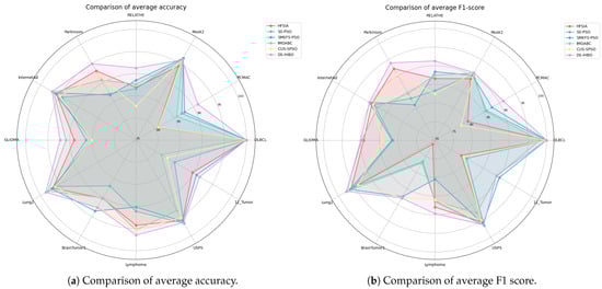
Figure 6. Comparison between DS-IHBO and other algorithms in average accuracy and F1 score visualization.

The Friedman test at the 0.05 significance level and the Finner test with an $\alpha$ value of 0.05 are employed to validate the performance of the proposed algorithm. Table 13 and Table 14 present the test results for the six algorithms, where DS-IHBO is selected as the reference method. In the tables, a smaller p-value from the Friedman test indicates higher confidence in the superiority of an algorithm over the others, while a smaller ranking value denotes superior performance across all datasets. The Friedman test results reveal that DS-IHBO achieved the lowest ranking value, significantly outperforming the other five comparative algorithms with statistical significance. The Finner test results indicate no significant difference between DS-IHBO and SMEFS-PSO, but DS-IHBO is significantly superior to the other four comparative algorithms. To strengthen the evidence for pairwise comparisons and quantify the magnitude of differences, the Wilcoxon signed-rank test is further performed in Table 15 and Table 16, and effect sizes are calculated to assess the practical significance of the differences. DS-IHBO is significantly superior to the aforementioned four algorithms in both accuracy and F1 score, with all effect sizes being highly significant. Although there are no statistically significant differences in classification performance between DS-IHBO and SMEFS-PSO, DS-IHBO showed better balance when considering the comprehensive objectives of FS. Subsequent experiments demonstrate that under comparable classification performance, DS-IHBO achieved higher computational efficiency and better feature dimensionality reduction performance.

Table 13. Friedman and Finner test results obtained by six algorithms (Acc).

Algorithms	Friedman Test			Finner Test
	Rank	p-Value		Adjusted p-Value	Significance (p < 0.05)
HFSIA	5.08			0.0008	Yes
SS-PSO	4.08			0.0042	Yes
SMEFS-PSO	2.92	$7.6\times {10}^{-6}$		0.0715	No
IMOABC	3.83			0.0121	Yes
CUS-SPSO	3.33			0.0236	Yes
DS-IHBO	1.75	—		—	—

Table 14. Friedman and Finner test results obtained by six algorithms (F1).

Algorithms	Friedman Test			Finner Test
	Rank	p-Value		Adjusted p-Value	Significance (p < 0.05)
HFSIA	5.50			0.0002	Yes
SS-PSO	4.58			0.0011	Yes
SMEFS-PSO	2.83	$8.0\times {10}^{-7}$		0.0632	No
IMOABC	3.50			0.0089	Yes
CUS-SPSO	4.00			0.0053	Yes
DS-IHBO	1.58	—		—	—

Table 15. Wilcoxon signed-rank test results obtained by six algorithms (Acc).

Algorithms	MSHRO vs.
	${\mathit{R}}^{\mathbf{+}}$	${\mathit{R}}^{\mathbf{-}}$	p-Value	Effect Size	Significance
HFSIA	78	0	0.0020	0.8421	Yes
SS-PSO	65	1	0.0078	0.7959	Yes
SMEFS-PSO	45	21	0.0746	0.2887	No
IMOABC	58	8	0.0117	0.7715	Yes
CUS-SPSO	63	3	0.0098	0.8036	Yes

Table 16. Wilcoxon signed-rank test results obtained by six algorithms (F1).

Algorithms	MSHRO vs.
	${\mathit{R}}^{\mathbf{+}}$	${\mathit{R}}^{\mathbf{-}}$	p-Value	Effect Size	Significance
HFSIA	82	0	0.0010	0.8563	Yes
SS-PSO	70	2	0.0049	0.8124	Yes
SMEFS-PSO	42	24	0.1098	0.2629	No
IMOABC	61	5	0.0146	0.7882	Yes
CUS-SPSO	67	5	0.0068	0.7982	Yes

Table 17 presents the imbalance robustness performance of six algorithms on binary classification problems. DS-IHBO consistently achieved optimal or co-optimal G-mean values across all six datasets. Notably, it significantly outperformed other algorithms on PCMAC, RELATHE, and Parkinson datasets (with improvements of 0.23%, 1.70%, and 1.21%, respectively). For complex datasets (e.g., RELATHE), DS-IHBO substantially exceeds the second-best algorithm (IMOABC). It also exhibits outstanding performance on noise-sensitive datasets (e.g., Parkinson). Furthermore, DS-IHBO maintained lower standard deviations on 5/6 datasets. Particularly on PCMAC, its standard deviation (0.79) is significantly lower than SS-PSO (1.97) and HFSIA (2.08), demonstrating enhanced algorithmic robustness.

Table 17. Average G-mean values obtained by six algorithms (std).

Datasets	HFSIA	SS-PSO	SMEFS-PSO	IMOABC	CUS-SPSO	DS-IHBO
DLBCL	100.00	100.00	100.00	97.33	100.00	100.00
	(0.00)	(0.00)	(0.00)	(0.42)	(0.00)	(0.00)
PCMAC	62.93	76.14	85.90	84.59	78.14	86.13
	(2.08)	(1.97)	(0.84)	(1.23)	(1.75)	(0.79)
Musk2	84.04	74.25	85.37	84.96	85.97	86.02
	(1.35)	(2.45)	(1.18)	(1.29)	(1.08)	(1.44)
RELATHE	74.06	74.89	78.22	86.51	82.12	88.21
	(2.14)	(2.08)	(1.73)	(0.86)	(1.38)	(0.71)
Parkinson	89.59	65.19	88.94	69.21	86.93	90.80
	(1.05)	(3.21)	(3.45)	(2.89)	(1.16)	(1.12)
InternetAd	74.22	76.60	77.81	77.01	77.34	77.81
	(2.03)	(1.47)	(1.86)	(1.59)	(1.52)	(1.43)

(2) Convergent curves of fitness value: As shown in Figure 7 and Figure 8, DS-IHBO exhibits rapid convergence in early iterations. For example, it achieves over 90% accuracy on the PCMAC dataset within 50 generations, and its convergence curves remain smooth in later iterations for datasets like RELATHE and Lymphoma. Theoretically, this performance stems from the synergy of its three modules: Module I narrows the search space via dimensionality reduction to lay the foundation for fast convergence; Module II maintains population diversity and balances exploration-exploitation through asymmetric initialization and adaptive differential operators, avoiding premature convergence to local optima; Module III reduces redundant evaluations on the original dataset to sustain convergence efficiency. To highlight the advantages of dynamic surrogate technology, DS-IHBO is compared with two baseline algorithms: (1) Static surrogate-based methods (e.g., CUS-SPSO, SMEFS-PSO) rely on fixed surrogate units, which easily introduce evaluation bias due to data distribution changes. For instance, CUS-SPSO shows obvious fitness discrepancies between training and test sets on the USPS dataset, leading to overfitting—while DS-IHBO’s dynamic surrogate updates effectively capture feature interactions and avoid such issues. (2) Surrogate-free EAs (e.g., HFSIA, IMOABC) require full-sample fitness evaluation, significantly increasing computational cost. For example, DS-IHBO’s runtime on PCMAC is only 19.3% of SMEFS-PSO’s. Further, HFSIA fails to maintain population diversity and falls into local optima on the GLIOMA dataset due to resource-intensive full-sample evaluations, whereas DS-IHBO avoids this via surrogate-assisted rapid exploration.

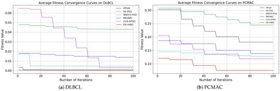
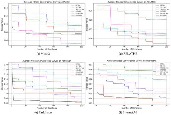
Figure 7. Evolution curves on the first six datasets.

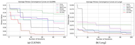
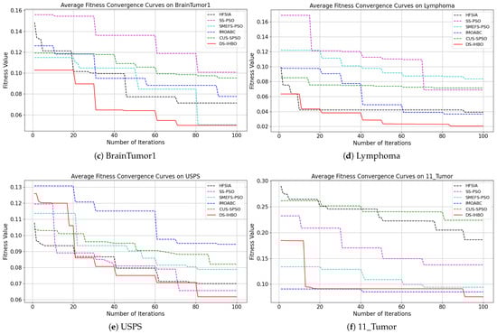
Figure 8. Evolution curves on the last six datasets.

(3) $d^{\ast }$ and $t^{\ast }$ values: Analysis of feature subset size (Table 18): (1) DS-IHBO selects the smallest feature subsets in half of the datasets; (2) HFSIA selects fewer features primarily due to its fixed filter threshold (200 features). Although achieving compact subsets, HFSIA exhibits inferior classification performance and imbalance robustness; (3) IMOABC attains the minimal feature count on PCMAC and Lung2, likely attributable to its tri-objective optimization framework: feature error rate minimization, feature subset proportion reduction, and inter-feature distance maximization.

Table 18. Average $d^{\ast }$ values obtained by six algorithms.

Datasets	HFSIA	SS-PSO	SMEFS-PSO	IMOABC	CUS-SPSO	DS-IHBO
DLBCL	11	166	351	153	2378	60
PCMAC	233	58	1005	54	1529	218
Musk2	86	133	109	67	100	83
RELATHE	220	295	520	281	2059	212
Parkinson	77	89	68	177	292	132
InternetAd	152	244	324	172	791	130
GLIOMA	57	358	51	180	1956	140
Lung2	95	324	430	20	1466	175
BrainTumor1	75	94	617	405	2679	67
Lymphoma	46	100	346	331	1746	99
USPS	88	93	115	90	101	82
11_Tumor	31	385	417	50	5095	116

To analyze the trade-off between performance gains and computational efficiency, the $t^{\ast }$ values of these algorithms are compared in Table 19. Key observations include (1) DS-IHBO demonstrates significantly lower $t^{\ast }$ values (computation time) than competitors on 10/12 datasets, owing to its efficient dynamic surrogate assistance. While not dominant on Musk2 and PCMAC, it maintains superior accuracy, F1 score, and G-mean; (2) HFSIA, SMEFS-PSO, and IMOABC—integrating filter-surrogate hybrid techniques—incur lower computational costs than pure evolutionary or surrogate methods. Notably, SMEFS-PSO’s local search phase introduces overhead in high-dimensional spaces, causing efficiency variance across scenarios; (3) CUS-SPSO exhibits suboptimal runtime performance versus peers, resulting from computation-intensive operations: particle selection strategies at each iteration increasing search complexity; pairwise feature correlation calculations during updates, particularly costly in high-dimensional data.

Table 19. Average $t^{\ast }$ values obtained by six algorithms (unit: s).

Datasets	HFSIA	SS-PSO	SMEFS-PSO	IMOABC	CUS-SPSO	DS-IHBO
DLBCL	33.03	221.26	300.26	131.68	881.27	20.58
PCMAC	3535.59	1748.10	1066.40	7393.55	23,940.00	2326.07
Musk2	1564.88	3598.00	8963.38	5852.29	21,123.44	3443.67
RELATHE	1785.32	7493.96	5256.66	5207.21	17,400.00	625.06
Parkinson	269.37	505.99	2009.54	285.61	5917.71	145.90
InternetAd	1724.58	3470.73	6152.37	7407.29	29,698.58	882.81
GLIOMA	33.49	65.09	207.08	65.39	754.29	29.77
Lung2	67.03	206.45	100.20	185.13	399.00	34.87
BrainTumor1	44.63	119.96	302.04	119.71	2007.67	26.64
Lymphoma	58.54	115.38	166.63	3922.37	2461.98	23.54
USPS	18,901.99	7362.30	9510.02	12,917.18	26,895.96	6872.09
11_Tumor	71.37	677.73	554.07	2358.32	1122.00	48.37

4.8. Parameter Sensitivity Analysis

The performance of the dynamic surrogate-assisted model depends significantly on two key parameters: the number of iterations $T_s$ during the surrogate evaluation phase and the surrogate unit update trigger threshold $T_n$. To determine the optimal parameter configuration, a comprehensive sensitivity analysis is conducted on these two parameters.

4.8.1. Parameter of Surrogate Model Iteration Count ($T_s$)

Five different values of $T_s$ (0, 25, 50, 75 and 100) are tested to evaluate the impact of the surrogate model’s iteration count on algorithm performance. $T_s$ = 0 indicates no use of the surrogate model at all, while higher $T_s$ values correspond to longer surrogate evaluation phases. Analysis of F1 score boxplots (Figure 9) reveals that on datasets such as DLBCL, PCMAC, and Musk2, $T_s$ = 75 achieved the best F1 scores. Its median value is significantly higher than those of other settings. Particularly on the DLBCL dataset, $T_s$ = 75 yielded an excellent F1 score of nearly 99%, significantly outperforming $T_s$ = 0 (no surrogate model) at 96%. This improvement is attributed to the surrogate model’s mechanism for handling imbalanced classes. $T_s$ = 75 generally exhibited smaller variance across most datasets, indicating superior algorithm stability at this setting. In contrast, $T_s$ = 0 (no surrogate model) showed larger performance fluctuations on many datasets. Performance showed a significant upward trend as $T_s$ increased from 0 to 75. However, when $T_s$ = 100, performance degradation is observed on some datasets, suggesting that an excessively long surrogate evaluation phase may introduce errors. Runtime analysis (Figure 10) highlights crucial computational efficiency characteristics: $T_s$ = 0 incurred the longest runtime, exceeding 10,000 s on large-scale complex datasets like PCMAC and Musk2. $T_s$ = 75 achieved favorable time efficiency on most datasets, reducing runtime by 60% to 80% compared with $T_s$ = 0. The runtime exhibited a steady decreasing trend from $T_s$ = 0 to $T_s$ = 100. Balancing the impact on F1 performance and runtime, $T_s$ = 75 is ultimately set to 75.

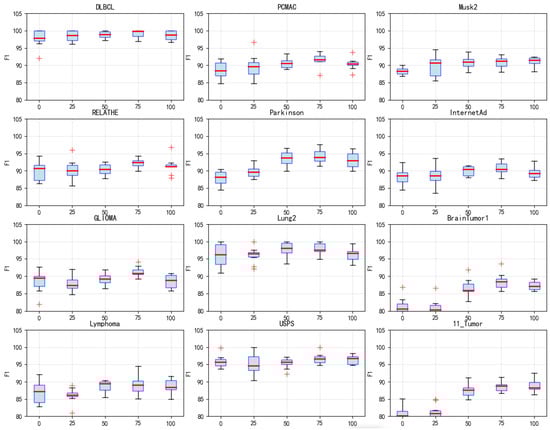
Figure 9. Box plots of F1 values obtained by DS-IHBO under different $T_s$ values.

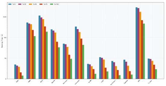
Figure 10. Running time of DS-IHBO under different $T_s$ values.

4.8.2. Dynamic Surrogate Switching Parameter ($T_n$)

Three different values of $T_n$ (5, 6, and 7) are tested to evaluate the impact of surrogate unit update frequency on algorithm performance. The comprehensive performance analysis (Figure 11) shows that $T_n$ = 6 achieved the highest accuracy rates on most datasets. Its accuracy advantage is particularly pronounced on complex datasets such as DLBCL and PCMAC. $T_n$ = 6 demonstrated the most balanced performance in terms of F1 score, maintaining high performance levels across all datasets. $T_n$ = 5 triggered updates too frequently, potentially causing excessive switching between surrogate units and adversely affecting convergence stability. $T_n$ = 7 triggered updates too infrequently, which might result in delayed responses to rapid environmental changes, potentially missing optimal opportunities for surrogate unit switching. $T_n$ = 6 exhibited a good balance in runtime. It avoided the computational burden associated with overly frequent updates ($T_n$ = 5) and mitigated the risk of slower convergence caused by delayed updates ($T_n$ = 7). $T_n$ = 6 provides an appropriate update frequency. It enables timely switching to a more suitable surrogate unit when the algorithm becomes trapped in local optimum. This moderate update frequency ensures the surrogate model adapts effectively to environmental changes during the search process while reducing computational cost.

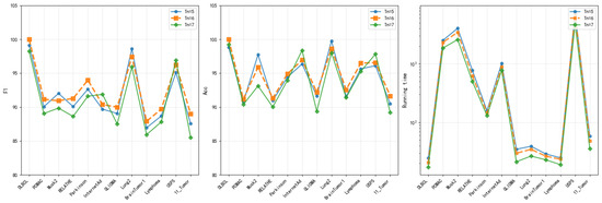
Figure 11. Acc, F1, and running time of DS-IHBO under different $T_n$ values.

The dynamic surrogate-assisted DS-IHBO demonstrates significant improvements over IHBO in classification accuracy, imbalance handling, and computational efficiency. This enhancement stems from four key mechanisms: (1) incorporating full-sample evaluation after 70% of maximum iterations ($0.75·T_m$) guarantees the final feature subset’s classification quality; (2) the adaptive surrogate selection mechanism continuously updates the most appropriate surrogate model during evolution, maintaining prediction reliability and boosting performance; (3) surrogate sample reduction substantially decreases training set dimensions, dramatically lowering individual evaluation costs; and (4) integrated adaptive KNN with minority-focused sampling prioritizes underrepresented classes during surrogate construction, effectively addressing class imbalance while strengthening minority class recognition.

5. Conclusions and Discussion

5.1. Conclusions

DS-IHBO, an enhanced FS approach derived from the IHBO algorithm, is presented in this paper. The proposed method integrates a dynamic surrogate-assisted mechanism with the IHBO algorithm to address the challenges of high-dimensional imbalanced FS while optimizing the search capability of HBO. Through strategic partitioning of complete sample sets into smaller surrogate units, our approach achieves a substantial reduction in computational overhead for fitness evaluation. Furthermore, the ensemble system continuously refines its surrogate units by comparing predicted and actual fitness values, thereby maintaining high prediction accuracy throughout the optimization process. The performance of our proposed FS method is assessed through comparative analysis with five EAs-based FS techniques (HFSIA, SS-PSO, SMEFS-PSO, IMOABC, and CUS-SPSO), which represent diverse strategies including high-dimensional processing, imbalance handling, surrogate modeling, and correlation-guided selection. Comparative analysis revealed that the DS-IHBO method consistently evolves high-quality and complementary feature subsets with superior classification accuracy while maintaining significantly lower computational overhead compared with competing approaches. Compared with IHBO without a dynamic surrogate, DS-IHBO achieved higher $Acc$ values and lower $t^{\ast }$ values on all datasets, as well as the highest F1 scores and G-mean values. These results significantly verify the efficiency and robustness of the algorithm. In summary, the proposed approach effectively enhances the HBO algorithm’s FS capability, yielding optimal feature combinations for classification tasks.

5.2. Limitations and Future Work

This paper primarily employs swarm intelligence algorithms to identify optimal feature subsets. Although the proposed DS-IHBO algorithm enhances the exploration of the search space and prevents entrapment in local optima, its convergence accuracy requires further improvement. Future research directions will include (1) expanding the application of the DS-IHBO algorithm to other high-dimensional optimization scenarios (e.g., image classification with high-resolution feature maps) to verify its generalizability; (2) exploring the integration of the proposed method with more advanced surrogate models (such as hybrid surrogate models) to further improve the efficiency of high-dimensional FS.

References

- Tudisco, A.; Volpe, D.; Ranieri, G.; Curato, G.; Ricossa, D.; Graziano, M.; Corbelletto, D. Evaluating the computational advantages of the variational quantum circuit model in financial fraud detection. IEEE Access 2024, 12, 102918–102940. [Google Scholar] [CrossRef]
- Fu, G.H.; Wang, J.B.; Lin, W. An adaptive loss backward feature elimination method for class-imbalanced and mixed-type data in medical diagnosis. Chemom. Intell. Lab. Syst. 2023, 236, 104809. [Google Scholar] [CrossRef]
- Nssibi, M.; Manita, G.; Chhabra, A.; Mirjalili, S.; Korbaa, O. Gene selection for high dimensional biological datasets using hybrid island binary artificial bee colony with chaos game optimization. Artif. Intell. Rev. 2024, 57, 51. [Google Scholar] [CrossRef]
- Arafah, M.; Phillips, I.; Adnane, A.; Hadi, W.; Alauthman, M.; Al-Banna, A.K. Anomaly-based network intrusion detection using denoising autoencoder and Wasserstein GAN synthetic attacks. Appl. Soft Comput. 2025, 168, 112455. [Google Scholar] [CrossRef]
- Barbieri, M.C.; Grisci, B.I.; Dorn, M. Analysis and comparison of feature selection methods towards performance and stability. Expert Syst. Appl. 2024, 249, 123667. [Google Scholar] [CrossRef]
- Li, M.; Zhao, Y.; Zhang, F.; Luo, B.; Yang, C.; Gui, W.; Chang, K. Multi-scale feature selection network for lightweight image super-resolution. Neural Netw. 2024, 169, 352–364. [Google Scholar] [CrossRef] [PubMed]
- Sharif, M.; Tanvir, U.; Munir, E.U.; Khan, M.A.; Yasmin, M. Brain tumor segmentation and classification by improved binomial thresholding and multi-features selection. J. Ambient Intell. Humaniz. Comput. 2024, 15, 1063–1082. [Google Scholar] [CrossRef]
- Nguyen, B.H.; Xue, B.; Zhang, M. A constrained competitive swarm optimizer with an SVM-based surrogate model for feature selection. IEEE Trans. Evol. Comput. 2024, 28, 2–16. [Google Scholar] [CrossRef]
- Hakami, A. Strategies for overcoming data scarcity, imbalance, and feature selection challenges in machine learning models for predictive maintenance. Sci. Rep. 2024, 14, 9645. [Google Scholar] [CrossRef]
- Kim, J.; Kang, J.; Sohn, M. Ensemble learning-based filter-centric hybrid feature selection framework for high-dimensional imbalanced data. Knowl.-Based Syst. 2021, 220, 106901. [Google Scholar] [CrossRef]
- Luo, X.; Chen, J.; Yuan, Y.; Wang, Z. Pseudo gradient-adjusted particle swarm optimization for accurate adaptive latent factor analysis. IEEE Trans. Syst. Man Cybern. Syst. 2024, 54, 2213–2226. [Google Scholar] [CrossRef]
- Qi, W.; Zhang, N.; Zong, G.; Su, S.F.; Yan, H.; Yeh, R.H. Event-triggered SMC for networked Markov jumping systems with channel fading and applications: Genetic algorithm. IEEE Trans. Cybern. 2023, 53, 6503–6515. [Google Scholar] [CrossRef] [PubMed]
- Hou, Y.; Guo, X.; Han, H.; Wang, J.; Du, Y. Adaptive ant colony optimization algorithm based on real-time logistics features for instant delivery. IEEE Trans. Cybern. 2024, 54, 6358–6370. [Google Scholar] [CrossRef] [PubMed]
- Zhang, L.; Chen, X. Elite-driven grey wolf optimization for global optimization and its application to feature selection. Swarm Evol. Comput. 2025, 92, 101795. [Google Scholar] [CrossRef]
- Yu, F.; Yin, L.; Zeng, B.; Lu, C.; Xiao, Z. A self-learning discrete artificial bee colony algorithm for energy-efficient distributed heterogeneous L-R fuzzy welding shop scheduling problem. IEEE Trans. Fuzzy Syst. 2024, 32, 3753–3764. [Google Scholar] [CrossRef]
- Sadeeq, H.T. Cauchy Operator Boosted Artificial Rabbits Optimization for Solving Power System Problems. Eng 2025, 6, 174. [Google Scholar] [CrossRef]
- Sun, L.; Sun, S.; Ding, W.; Huang, X.; Fan, P.; Li, K.; Chen, L. Feature selection using symmetric uncertainty and hybrid optimization for high-dimensional data. Int. J. Mach. Learn. Cybern. 2023, 14, 4339–4360. [Google Scholar] [CrossRef]
- Ye, Z.; Ma, L.; Chen, H. A hybrid rice optimization algorithm. In Proceedings of the 11th International Conference on Computer Science & Education (ICCSE), Nagoya, Japan, 23–25 August 2016; pp. 169–174. [Google Scholar]
- Ye, Z.; Luo, J.; Zhou, W.; Wang, M.; He, Q. An ensemble framework with improved hybrid breeding optimization-based feature selection for intrusion detection. Future Gener. Comput. Syst. 2024, 151, 124–136. [Google Scholar] [CrossRef]
- Mei, M.; Zhang, S.; Ye, Z.; Wang, M.; Zhou, W.; Yang, J.; Zhang, J.; Yan, L.; Shen, J. A cooperative hybrid breeding swarm intelligence algorithm for feature selection. Pattern Recognit. 2026, 169, 111901. [Google Scholar] [CrossRef]
- Wei, C.; Peng, B.; Li, C.; Liu, Y.; Ye, Z.; Zuo, Z. A two-stage optimized robust kernel density estimation for Bayesian classification with outliers. Int. J. Mach. Learn. Cybern. 2025, 1–25. [Google Scholar] [CrossRef]
- Brownlee, A.E.I.; Regnier-Coudert, O.; McCall, J.A.W.; Massie, S.; Stulajter, S. An application of a GA with Markov network surrogate to feature selection. Int. J. Syst. Sci. 2013, 44, 2039–2056. [Google Scholar] [CrossRef]
- Chen, K.; Xue, B.; Zhang, M.; Zhou, F. Correlation-guided updating strategy for feature selection in classification with surrogate-assisted particle swarm optimization. IEEE Trans. Evol. Comput. 2022, 26, 1015–1029. [Google Scholar] [CrossRef]
- Nguyen, H.B.; Xue, B.; Andreae, P. Surrogate-model based particle swarm optimisation with local search for feature selection in classification. In Applications of Evolutionary Computation; Squillero, G., Burelli, P., Eds.; Springer International Publishing: Cham, Switzerland, 2017; pp. 487–505. [Google Scholar]
- Song, X.F.; Zhang, Y.; Gong, D.W.; Gao, X.Z. A fast hybrid feature selection based on correlation-guided clustering and particle swarm optimization for high-dimensional data. IEEE Trans. Cybern. 2022, 52, 9573–9586. [Google Scholar] [CrossRef] [PubMed]
- Al-Rawashdeh, R.; Aljughaiman, A.; Albuali, A.; Alsenani, Y.; Alnaeem, M. Enhancing DoS detection in WSNs using enhanced ant colony optimization algorithm. IEEE Access 2024, 12, 134651–134671. [Google Scholar] [CrossRef]
- Miao, F.; Wu, Y.; Yan, G.; Si, X. A memory interaction quadratic interpolation whale optimization algorithm based on reverse information correction for high-dimensional feature selection. Appl. Soft Comput. 2024, 164, 111979. [Google Scholar] [CrossRef]
- Ahadzadeh, B.; Abdar, M.; Safara, F.; Khosravi, A.; Menhaj, M.B.; Suganthan, P.N. SFE: A simple, fast, and efficient feature selection algorithm for high-dimensional data. IEEE Trans. Evol. Comput. 2023, 27, 1896–1911. [Google Scholar] [CrossRef]
- Pan, J.S.; Shi, H.J.; Chu, S.C.; Hu, P.; Shehadeh, H.A. Parallel Binary Rafflesia Optimization Algorithm and Its Application in Feature Selection Problem. Symmetry 2023, 15, 1073. [Google Scholar] [CrossRef]
- Li, L.; Xuan, M.; Lin, Q.; Jiang, M.; Ming, Z.; Tan, K.C. An evolutionary multitasking algorithm with multiple filtering for high-dimensional feature selection. IEEE Trans. Evol. Comput. 2023, 27, 802–816. [Google Scholar] [CrossRef]
- Ying, W.; Wang, D.; Chen, H.; Fu, Y. Feature selection as deep sequential generative learning. ACM Trans. Knowl. Discov. Data 2024, 18, 1–21. [Google Scholar] [CrossRef]
- Pan, H.; Chen, S.; Xiong, H. A high-dimensional feature selection method based on modified Gray Wolf optimization. Appl. Soft Comput. 2023, 135, 110031. [Google Scholar] [CrossRef]
- Jiang, Z.; Zhang, Y.; Wang, J. A multi-surrogate-assisted dual-layer ensemble feature selection algorithm. Appl. Soft Comput. 2021, 110, 107625. [Google Scholar] [CrossRef]
- Gao, J.; Wang, Z.; Jin, T.; Cheng, J.; Lei, Z.; Gao, S. Information gain ratio-based subfeature grouping empowers particle swarm optimization for feature selection. Knowl.-Based Syst. 2024, 286, 111380. [Google Scholar] [CrossRef]
- Lin, H.; Wang, C.; Hao, Q. A novel personality detection method based on high-dimensional psycholinguistic features and improved distributed Gray Wolf optimizer for feature selection. Inf. Process. Manag. 2023, 60, 103217. [Google Scholar] [CrossRef]
- Song, X.; Jiang, Z.; Zhang, Y.; Peng, C.; Guo, Y. A surrogate-assisted multi-phase ensemble feature selection algorithm with particle swarm optimization in imbalanced data. IEEE Trans. Emerg. Top. Comput. Intell. 2025, 1–16. [Google Scholar] [CrossRef]
- Song, X.; Zhang, Y.; Gong, D.; Liu, H.; Zhang, W. Surrogate sample-assisted particle swarm optimization for feature selection on high-dimensional data. IEEE Trans. Evol. Comput. 2023, 27, 595–609. [Google Scholar] [CrossRef]
- Liu, S.; Wang, H.; Peng, W.; Yao, W. A Surrogate-Assisted Evolutionary Feature Selection Algorithm With Parallel Random Grouping for High-Dimensional Classification. IEEE Trans. Evol. Comput. 2022, 26, 1087–1101. [Google Scholar]
- Liu, S.; Wang, H.; Peng, W.; Yao, W. Surrogate-assisted evolutionary algorithms for expensive combinatorial optimization: A survey. Complex Intell. Syst. 2024, 10, 5933–5949. [Google Scholar] [CrossRef]
- Chu, S.C.; Yuan, X.; Pan, J.S.; Lin, B.S.; Lee, Z.J. A multi-strategy surrogate-assisted social learning particle swarm optimization for expensive optimization and applications. Appl. Soft Comput. 2024, 162, 111876. [Google Scholar] [CrossRef]
- Yu, K.; Sun, S.; Liang, J.; Chen, K.; Qu, B.; Yue, C.; Suganthan, P.N. A Space Transformation-Based Multiform Approach for Multiobjective Feature Selection in High-Dimensional Classification. IEEE Trans. Syst. Man Cybern. Syst. 2024, 54, 7305–7317. [Google Scholar]
- Hu, P.; Zhu, J. A filter-wrapper model for high-dimensional feature selection based on evolutionary computation. Appl. Intell. 2025, 55, 581. [Google Scholar] [CrossRef]
- Gong, H.; Li, Y.; Zhang, J.; Zhang, B.; Wang, X. A new filter feature selection algorithm for classification task by ensembling Pearson correlation coefficient and mutual information. Eng. Appl. Artif. Intell. 2024, 131, 107865. [Google Scholar] [CrossRef]
- Wang, Q.; Jiang, H.; Ren, J.; Liu, H.; Wang, X.; Zhang, B. An intrusion detection algorithm based on joint symmetric uncertainty and hyperparameter optimized fusion neural network. Expert Syst. Appl. 2024, 244, 123014. [Google Scholar] [CrossRef]
- Ramírez-Gallego, S.; Lastra, I.; Martínez-Rego, D.; Bolón-Canedo, V.; Benítez, J.M.; Herrera, F.; Alonso-Betanzos, A. Fast-mRMR: Fast minimum redundancy maximum relevance algorithm for high-dimensional big data. Int. J. Intell. Syst. 2017, 32, 134–152. [Google Scholar] [CrossRef]
- Liaw, L.C.M.; Tan, S.C.; Goh, P.Y.; Lim, C.P. A histogram SMOTE-based sampling algorithm with incremental learning for imbalanced data classification. Inf. Sci. 2025, 686, 121193. [Google Scholar] [CrossRef]
- Zhu, Y.; Li, W.; Li, T. A hybrid artificial immune optimization for high-dimensional feature selection. Knowl.-Based Syst. 2023, 260, 110111. [Google Scholar] [CrossRef]
- Li, J.; Luo, T.; Zhang, B.; Chen, M.; Zhou, J. IMOABC: An efficient multi-objective filter–wrapper hybrid approach for high-dimensional feature selection. J. King Saud Univ. Comput. Inf. Sci. 2024, 36, 102205. [Google Scholar] [CrossRef]
- Wang, H.; Li, G.; Wang, Z. Fast SVM classifier for large-scale classification problems. Inf. Sci. 2023, 642, 119136. [Google Scholar] [CrossRef]
Disclaimer/Publisher’s Note: The statements, opinions and data contained in all publications are solely those of the individual author(s) and contributor(s) and not of MDPI and/or the editor(s). MDPI and/or the editor(s) disclaim responsibility for any injury to people or property resulting from any ideas, methods, instructions or products referred to in the content. |
© 2025 by the authors. Licensee MDPI, Basel, Switzerland. This article is an open access article distributed under the terms and conditions of the Creative Commons Attribution (CC BY) license (https://creativecommons.org/licenses/by/4.0/).