Enhanced Feature Engineering Symmetry Model Based on Novel Dolphin Swarm Algorithm

Abstract

This study addresses the challenges of high-dimensional data, such as the curse of dimensionality and feature redundancy, which can be viewed as an inherent asymmetry in the data space. To restore a balanced symmetry and build a more complete feature representation, we propose an enhanced feature engineering model (EFEM) that employs a novel dual-strategy approach. First, we present a symmetrical feature selection algorithm that combines an improved Dolphin Swarm Algorithm (DSA) with the Maximum Relevance–Minimum Redundancy (mRMR) criterion. This method not only selects an optimal, high-relevance feature subset, but also identifies the remaining features as a complementary, redundant subset. Second, an ensemble learning-based feature reconstruction algorithm is introduced to mine potential information from these redundant features. This process transforms fragmented, redundant information into a new, synthetic feature, thereby establishing a form of information symmetry with the selected optimal subset. Finally, the EFEM constructs a high-performance feature space by symmetrically integrating the optimal feature subset with the synthetic feature. The model’s superior performance is extensively validated on nine standard UCI regression datasets, with comparative analysis showing that it significantly outperforms similar algorithms and achieves an average goodness-of-fit of 0.9263. The statistical significance of this improvement is confirmed by the Wilcoxon signed-rank test. Comprehensive analyses of parameter sensitivity, robustness, convergence, and runtime, as well as ablation experiments, further validate the efficiency and stability of the proposed algorithm. The successful application of the EFEM in a real-world product demand forecasting task fully demonstrates its practical value in complex scenarios.

1. Introduction

1.1. Research Background and Challenges

Feature engineering is the process of transforming raw data into features that better represent the underlying problem. As an essential component of the data mining process, it bridges data cleaning and modeling, and is closely related to the performance of model algorithms. High-quality feature engineering can effectively improve data quality and reveal features that benefit algorithm models.

It is a key technology for improving the performance of machine learning models and has demonstrated enormous application value in fields such as healthcare, fintech, industrial IoT, intelligent recommendation, and autonomous driving. In the medical field, An et al. [1] reduced misdiagnosis rates by the automated extraction of critical interaction features to improve the diagnostic accuracy of acute appendicitis. Zhao et al. [2] proposed a model to simultaneously capture spatial and temporal features to improve portfolio management and trading decision-making performance. In industrial scenarios, Siemens [3] utilized vibration characteristics to achieve a 95% accuracy rate for fault warning. Research has shown that excellent feature engineering can improve model performance by 3–5 times compared to algorithm improvement, while reducing computational costs by 70% [4,5]. Behind these practical achievements, it is inseparable from the continuous breakthroughs and innovations in feature engineering methodology.

In recent years, feature engineering has made significant progress in many areas. In automated feature engineering, Abhyankar et al. [6] proposed a new automatic feature engineering framework that combines large language models with evolutionary search. Wang et al. [7] proposed an automatic feature engineering architecture based on reinforcement learning. In interpretability research, Verdonck et al. [8] emphasized the importance of feature engineering in improving the performance of machine learning models, and believed that carefully designed features can still greatly improve the performance of such models, while Duan et al. [9] used a graph structure and causal inference modules to automatically identify key causal nodes from transaction history, significantly reducing false positives. In cross-modality, progress includes Radford et al.’s [10] contrastive learning model, which outperformed the combination of a deep residual network and bidirectional Transformer encoder by 17% in cross-modal retrieval. Yu et al. [11] employed a time series autoencoder to significantly enhance industrial fault detection performance, achieving high F1-scores. Studies such as Da et al. [12] and Rieke et al. [13] demonstrated that federated learning frameworks can achieve feature processing and model performance (up to 98% of centralized training) with close approximation and stability. OpenAI [14] demonstrated GPT-4′s ability to generate business-usable features (with an adoption rate of 73%). This also extends to cutting-edge fields like federated learning, digital twins, and distributed systems, which are crucial for industrial IoT and smart grid applications [15,16,17,18,19].

Beyond automated and interpretable feature engineering, intelligent bio-inspired algorithms have emerged as a powerful tool to further enhance feature selection and optimization. Intelligent bionic algorithms also have many applications in feature engineering. Gulati et al. [20] developed a hierarchical feature engineering method combining nonlinear transformations and genetic algorithms with bootstrapped selection, boosting interpretable model performance while reducing dimensionality. Song et al. [21] proposed a surrogate sample-assisted particle swarm optimization hybrid feature selection algorithm, which effectively addressed high-dimensional feature selection problems while reducing computational costs through a collaborative sample partitioning and feature clustering mechanism. Ma et al. [22] proposed a two-stage hybrid ant colony optimization algorithm for high-dimensional feature selection, significantly improving search efficiency and feature selection performance on high-dimensional data. Saheed et al. [23] proposed a binary firefly algorithm-based feature selection method that achieved a 99.72% detection accuracy on high-dimensional datasets through a three-stage processing framework. Pethe et al. [24] proposed a bat optimization algorithm-based feature selection method that achieved a peak accuracy of 98.92% while effectively reducing feature dimensionality.

With the assistance of intelligent bionic algorithms, the quality of feature engineering is improved, and high-quality feature engineering is crucial to the success of regression analysis. Arroba et al. [25] constructed a highly information-based feature expression, reducing prediction error to an average of 3.98%. Research on regression analysis methods has demonstrated diversified development trends. Regarding traditional method optimization, Prokhorenkova et al. [26] developed the CatBoost-R algorithm, which substantially reduced overfitting risk in time series regression tasks through ordered target encoding. In ensemble learning, Lim et al. [27] designed the Temporal Fusion Transformer, which reduced MAE by 23% in multivariate time series regression problems.

Beyond traditional industrial applications, recent advancements in structural health monitoring (SHM) and vibration-based damage detection have also demonstrated that data-driven and optimization-based approaches play a crucial role in identifying hidden structural defects and predicting failures. In particular, machine learning and bio-inspired algorithms have been widely applied in tasks such as beam crack detection, joint-induced vibration analysis, and defect prediction, showing strong potential for enhancing reliability in mechanical and civil engineering systems [28,29,30,31,32,33]. These studies highlight the broader applicability of advanced feature selection and optimization techniques beyond traditional industrial fault detection. Inspired by this line of research, the proposed semi-supervised feature selection framework in this study may also provide valuable insights for vibration-based SHM applications, further underscoring the generality and adaptability of the method.

The above research status indicates that feature engineering has become a core driving force for improving the performance of machine learning models, especially in regression analysis and prediction tasks, where it demonstrates significant value. These advances provide important insights for this study. First, there is an urgent need to develop a hybrid feature selection framework that integrates swarm intelligence and statistical criteria to balance automation efficiency and business interpretability. Second, feature optimization for regression tasks needs to consider both global correlation and local redundancy simultaneously. Finally, algorithm design should focus on reducing computational complexity to adapt to industrial-level application scenarios.

1.2. Gaps in Existing Research

Although feature engineering technology has made significant progress, there are still many problems and challenges in feature engineering, as follows:

(1)

Insufficient robustness of feature selection algorithms

Existing feature selection methods, such as those based on statistics, information theory, or embedded algorithms, are sensitive to data noise. When the data distribution changes or there are outliers, the stability of the selected feature subset is poor. Most studies only focus on the accuracy of feature selection and neglect the stability evaluation of algorithms in noisy environments [34,35,36,37].

(2)

Insufficient utilization of redundant features

Traditional feature selection methods, such as filters, wrappers, and embedded methods, typically reduce data dimensionality and improve model efficiency by eliminating redundant or low-information features based on their correlation or importance to the target variable. However, these methods have a key limitation: features marked as “redundant” are not completely useless, but may contain supplementary information or potential patterns indirectly related to the target variable. Directly discarding these features may lead to information loss, especially in high-dimensional or complex scenarios, where the synergistic effect of features may significantly affect model performance [38,39,40].

1.3. Motivation and Contributions

To address these issues, this study proposes a new feature construction paradigm that synthesizes low-dimensional but informative features by integrating valuable information from redundant features. This method not only reduces the number of features and alleviates the curse of dimensionality, but also avoids the inherent information waste in traditional feature selection, thereby improving model efficiency while fully utilizing the potential of data. This method has significant prospects in handling high-dimensional data, resource-constrained scenarios, and tasks that require strong interpretability.

The main contributions of this study are as follows: A dolphin swarm feature selection algorithm based on the theory of maximum correlation and minimum redundancy is proposed, specifically designed for regression datasets. Through this algorithm, important feature subsets and potential redundant feature subsets are identified. Considering that redundant feature subsets may contain key information, ensemble learning methods are adopted, where multiple machine learning models process these redundant features and generate new feature subsets. Subsequently, the model with the best performance is selected for secondary training to construct a new composite feature that fully preserves all the basic information in the redundant features. By combining the features selected by the Dolphin Swarm Algorithm with the newly constructed features, the final feature subset is formed to complete the entire feature engineering process. The proposed method is ultimately validated through regression algorithms, and comparative experiments and statistical analysis demonstrate its superior performance compared to other similar methods.

1.4. Structure and Organization

The content of this study is organized as follows: Section 2 explains the basic theory of feature engineering and predictive regression; Section 3 proposes an improved Dolphin Swarm Algorithm and constructs the overall framework of feature engineering; and Section 4 comprehensively validates the effectiveness of the proposed EFEM algorithm. We conduct comparative evaluations against various advanced feature selection algorithms on nine UCI regression datasets. Through ablation studies, statistical tests, and convergence analysis, we quantify the contributions of each algorithm component and verify the reliability of its conclusions. We also conduct parameter sensitivity analysis and noise robustness tests. Finally, we apply the algorithm to a real-world product demand forecasting task. Section 5 summarizes the research results, explains the innovations, and looks forward to future research directions. The organizational structure of the full paper is shown in Figure 1.

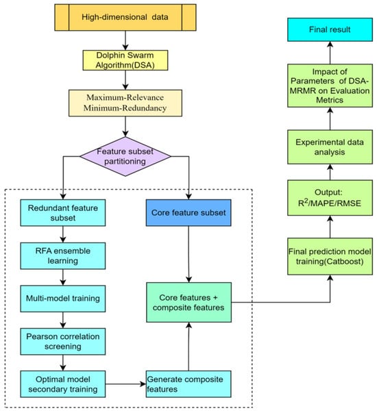
Figure 1. Research framework diagram.

2. Background

2.1. Feature Engineering

Feature engineering is the core process of machine learning, which improves model prediction performance, reduces computational complexity, alleviates dimensional disaster, enhances generalization ability, prevents overfitting, and improves interpretability by optimizing feature expression, reducing noise and redundant features, and screening key features, thereby comprehensively improving model performance and efficiency [41].

Feature engineering includes feature selection and feature construction, which are indispensable and important parts of the feature engineering process. Feature selection refers to the process of selecting the most relevant and valuable subset of features from an original feature set. Its core goal is to reduce data dimensionality, decrease computational overhead, improve model performance, and enhance the interpretability of results. By removing redundant and irrelevant features, feature selection can help machine learning models learn key patterns in data more efficiently and improve generalization ability.

Feature construction refers to the process of creating new, more predictive features by transforming, combining, or decomposing original features. Its core goal is to enhance the representation ability of features, mine hidden relationships in data, and improve the expression ability of models. Unlike feature selection, feature construction does not simply select existing features, but creates new features through mathematical transformations or domain knowledge, making it easier for machine learning algorithms to discover potential patterns in data. Feature construction can be either explicit (based on domain knowledge) or implicit (generated through algorithms) [42].

2.2. Regression and Predictive

Regression is an important branch of supervised learning, whose core feature is that the target variable is a continuous numerical value rather than a discrete class label. This requires different methods to be used for modeling and optimizing regression problems [43]. Traditionally, regression analysis is based on statistical methods such as linear regression, which assumes a linear relationship between input features and output variables and fits the model by minimizing prediction error. When there is a nonlinear relationship in the data, polynomial regression or machine learning methods can be used to enhance the expressive power. In addition, regression problems often face challenges such as overfitting, noisy data, and feature collinearity, so regularization techniques such as ridge regression and Lasso regression are widely used to improve model robustness. The evaluation of regression models typically uses metrics such as mean squared error ($MSE$), mean absolute error ($MAE$), and the coefficient of determination ($R^2$) to measure prediction accuracy.

The core purpose of regression problems is to predict continuous numerical values, thereby providing a quantitative basis for decision making. In practical applications, regression models are widely used in scenarios such as housing price prediction, temperature trend analysis, stock price trends, and sales forecasting.

Modern machine learning provides various modeling tools for regression problems. Traditional methods include linear regression, polynomial regression, and regularized regression (such as ridge regression and Lasso regression), which are suitable for linear or mildly nonlinear data. For more complex nonlinear relationships, support vector regression (SVR) maps data to high-dimensional space through kernel functions, while ensemble methods such as decision trees and random forests can automatically capture interactions between features [44].

3. Research Methodology

Given the gap in feature engineering research mentioned in Section 1.3, this study proposes our solutions to address these issues.

3.1. Principle of Standard Dolphin Swarm Algorithm

The Dolphin Swarm Algorithm (DSA) simulates the cooperative hunting behavior of dolphin groups, leveraging acoustic communication and dynamic capture mechanisms, demonstrating unique advantages in optimization problems. Its swarm intelligence collaboration can efficiently share information and avoid premature convergence, dynamically adjusting strategies to balance exploration and development capabilities, making it suitable for handling high-dimensional and nonlinear problems. Compared to particle swarm optimization and genetic algorithms, it is more adaptable between global search and local refinement, making it especially suitable for complex scenarios such as path planning and parameter optimization. However, the computational cost may increase with an increase in population size. We need to use its advantage for feature selection.

In this article, $U$ is defined as the set of all samples and $A$ is defined as the set of all features, with $S$ being a subset of $A$ (i.e., $S\subseteq A$). The target variable is denoted by $y$, The number of samples is represented by $\left|U\right|$ and the number of features is represented by $\left|A\right|$. The basic principles of the Dolphin Swarm Algorithm are shown in Algorithm 1.

Algorithm 1. Original Dolphin Swarm Algorithm

Input: Regression Dataset, Parameters, Population size, Maximum iterations, Objective function. Output: Optimal Feature Subset: Step 1: Each dolphin in the population is represented by a binary vector $P=\left[p_1,p_2,\right.\dots ,\left.p_m\right]$, where $\left|A\right|$ is the total number of features. $p_i=1$ indicates that the $i$-th feature is selected, and $p_i=0$ indicates it is not selected. Step 2: Randomly generate $N$ initial individuals in the population. Step 3: Use the binary vector $P$ to extract the selected features subsets $S$ from $A$. Step 4: Train a regression model (e.g., linear regression, random forest) using the selected features subsets $S$ and the target $y$. Step 5: Use the objective function $f\left(x_i\right)$ compute the fitness value. Step 6: Randomly update individuals based on a global best solution. $P^{t+1}=P^t+a\cdot \left(S-P^t\right)+b\cdot \mu$ Step 7: Simulate local search behavior by refining individual solutions, such as flipping specific feature selection states. Step 8: Update the global best features subsets $S$ based on fitness values. Step 9: Record the best feature subset $S$ found so far. Step 10: Terminate the algorithm when the maximum number of iterations $T$ is reached or when the fitness value stabilizes.

Step 6 represents the weight for approaching the optimal solution, the weight for random perturbation, and the random perturbation term, which uses either Gaussian noise or uniform noise.

3.2. Maximum Relevance and Minimal Redundancy (mRMR) for Regression

Then, we introduce the maximum correlation and minimum redundancy. The Maximum Relevance–Minimum Redundancy (mRMR) model maximizes the correlation between features and the target variable while minimizing the redundancy between features, which can more effectively filter out feature subsets with strong discriminability. Therefore, this study proposes integrating the optimization criteria of mRMR into the Dolphin Swarm Algorithm, enhancing the global search capability using the biomimetic optimization mechanism of the DSA, and combining the information theory evaluation criteria of mRMR to enable the algorithm to maintain efficient search while accurately balancing the correlation and redundancy of features, thereby improving the robustness and interpretability of feature selection.

The Maximum Relevance–Minimum Redundancy (mRMR) framework is a feature selection methodology that balances the following two competing objectives: (1) Maximum Relevance, which prioritizes features with the strongest statistical association with the target variable, and (2) Minimum Redundancy, which minimizes information overlap among selected features to avoid redundancy. While mRMR is widely adopted in classification tasks using mutual information, its direct application to regression problems—where the target h is continuous—requires critical adaptations. This study addresses this gap by redesigning mRMR’s relevance metric for regression while retaining its core redundancy control mechanism.

In classification, mutual information measures nonlinear dependencies between discrete features and targets. However, regression tasks often involve linear relationships between continuous variables. To bridge this gap, we propose the following two key modifications:

(1)

Relevance Metric: Replace mutual information with the F-statistic, which quantifies the linear dependence between a feature $x_i$ and the continuous target $h$.

(2)

Redundancy Metric: Retain Pearson correlation to evaluate pairwise feature redundancy [45], ensuring computational efficiency and interpretability.

To operationalize the aforementioned adaptations for regression tasks, we formalize the mRMR framework through rigorously defined mathematical metrics. Specifically, the replacement of mutual information with the F-statistic and the retention of Pearson correlation are concretized as follows (the parameter descriptions in the formula are shown in Table 1):

Table 1. Symbol definition.

Symbol	Definition
$K$	Number of subgroups for h-binning
$n_k$	Sample size of subgroup $k$
${\overline{x}}_i$	Global mean of feature $x_i$
$\lambda$	Redundancy penalty coefficient

(1)

Feature Relevance via F-Statistic:

The F-statistic, chosen for its sensitivity to linear dependencies in continuous variables, quantifies the ratio of between-group variance to within-group variance. For a feature $x_i$ and target $h$, it is defined as follows:

$$F(x_i,h)={\displaystyle \frac{{\displaystyle {\sum }_{k=1}^K{n}_k}{\left({\overline{x}}_i^{\left(k\right)}-{\overline{x}}_i\right)}^2/\left(K-1\right)}{{\displaystyle {\sum }_{k=1}^K{\displaystyle {\sum }_{j=1}^{n_k}{\left(x_{ij}^{\left(k\right)}-{\overline{x}}_i^k\right)}^2/\left(N-K\right)}}}}$$

(1)

Since the target variable $h$ in the research datasets is continuous, it requires discretization through binning for actual computation.

(2)

Feature Redundancy via Pearson Correlation:

Redundancy between features $x_i$ and $x_j$ is measured as follows:

$$\rho \left(x_i,x_j\right)=\left|{\displaystyle \frac{Cov\left(x_i,x_j\right)}{{\sigma }_{x_i}{\sigma }_{x_j}}}\right|$$

(2)

The covariance $Cov(x_i,x_j)$ captures the co-variation trend between two features, while the standard deviations ${\sigma }_{x_i}$ and ${\sigma }_{x_j}$ perform normalization to eliminate scale effects. The absolute value ensures non-negative results. An R-value below 0.3 indicates low redundancy between features, while values above 0.7 suggest high redundancy requiring special attention.

(3)

mRMR Optimization Criterion:

The optimal feature subset $S$ maximizes relevance while minimizing redundancy, as follows:

$$\underset{S}{\max }\left[{\displaystyle \frac{1}{\left|S\right|}}{\displaystyle \sum _{x_i\in S}F\left(x_i,h\right)-\frac{\lambda }{{\left|S\right|}^2}{\displaystyle \sum _{x_i,x_j\in S}R\left(x_i,x_j\right)}}\right]$$

(3)

$\lambda$: Balances the trade-off between relevance and redundancy (default $\lambda$ = 1).

Traditional mRMR frameworks for classification fail to handle continuous targets due to their reliance on mutual information [46]. By integrating the F-statistic, our adaptation extends applicability to regression problems by replacing mutual information with the F-statistic for relevance assessment, enhances robustness through statistical significance testing, automatically filtering non-predictive features, maintains efficiency by leveraging ANOVA-based approximations for high-dimensional data, and preserves interpretability by keeping the redundancy term based on Pearson correlation.

3.3. Fitness Function

As can be seen from the previous section, the key to the Dolphin Swarm Algorithm is to define the fitness function. To this end, we define a new fitness function by combining the mRMR formula with reduction rate.

$$Fitness\left(S\right)=\alpha \left[{\displaystyle \frac{1}{\left|S\right|}}{\displaystyle \sum _{x_i\in S}F\left(x_i,h\right)-\frac{1}{{\left|S\right|}^2}{\displaystyle \sum _{x_i,x_j\in S}\rho \left(x_i,x_j\right)}}\right]+\beta \left(1-{\displaystyle \frac{\left|S\right|}{\left|A\right|}}\right)$$

(4)

In Formula (4), parameter $\alpha$ is used to balance the trade-off between the maximum relevance and minimum redundancy of the feature subset, while parameter $\beta$ controls the computational efficiency of feature selection.

${\displaystyle \frac{1}{\left|S\right|}}{\displaystyle \sum F\left(x_i,h\right)}$: Average relevance of selected features to the target $h$.

${\displaystyle \frac{1}{{\left|S\right|}^2}}{\displaystyle \sum \rho \left(x_i,x_j\right)}$: Average redundancy among selected features.

$\alpha$: Weight balancing relevance and redundancy.

${\displaystyle \frac{\left|S\right|}{\left|A\right|}}$: Ratio of selected features ($\left|S\right|$) to total original features ($A$).

$\beta$: Weight controlling the penalty for high dimensionality.

3.4. DSA–mRMR Algorithm for Feature Selection

In the previous chapters, the standard Dolphin Swarm Algorithm (DSA) achieved global search by simulating dolphin swarm intelligence. Based on the Maximum Relevance–Minimum Redundancy (mRMR) criterion, this section proposes a DSA–mRMR hybrid algorithm, which integrates the DSA’s search capability with mRMR’s feature evaluation criterion. The fitness function (Formula (4)) dynamically balances the correlation and redundancy of feature subsets.

Next, we propose a new mRMR-based Dolphin Swarm Algorithm for feature selection. The algorithm is shown in Algorithm 2.

Algorithm 2. A novel feature selection algorithm (DSA–mRMR)

Input: An information system, initial values of various parameters. Output: A feature subset S 1. Initialize a population of dolphins $N$, where each dolphin represents a binary vector $S=\left[s_1,s_2,\dots ,s_{\left|A\right|}\right.$, $s_i$ = 1 if the feature $s_i$ is selected else 0. 2. Compute Fitness for each dolphin using the Formula (4). 3. Calculate Adaptive Mutation Probability for the current iteration:

$P_{\mathrm{mut}}\left(t\right)=P_{mut}^{\min }+\left(P_{mut}^{\max }-P_{mut}^{\min }\right)\cdot e^{-\lambda \left(t/T_{\max }\right)}$

4. Individual Exploration(Mutation): For each dolphin, mutate each bit in its vector with the current adaptive probability $P_{mut}\left(t\right)$:

$s_i^{\prime }=\left\{\begin{array}{cc}1-s_i,\hfill & \mathrm{if} rand\left(\right)<p_{mut}\left(t\right)\hfill \\ s_i,\hfill & otherwise\hfill \end{array}\right.$

5. Move toward the current best solution: For each dolphin and for each bit $i$, update as:

$S_{k,i}^{t+1}=\left\{\begin{array}{cc}{S}_{best,i}^t,\hfill & with probability p_{\mathrm{reinforce}}\hfill \\ S_{k,i}^t,\hfill & otherwise\hfill \end{array}\right.$

6. Update best solution: $s_{best}^{t+1}=\arg \max Fitness(S)$ 7. Stop if maximum iterations reached $T_{\max }$ or fitness improvement < $\epsilon$ ($\epsilon$ = 10−5) and output the best subsets.

The initial mutation rate ($P_{mut}^{\max }=0.4$) is set high to encourage extensive exploration in the early search phase, allowing dolphins to radically alter their feature subsets.

The minimum rate ($P_{mut}^{\min }=0.05$) is set low to ensure that the algorithm stabilizes and finely exploits the most promising regions of the search space in later iterations.

The decay rate ($\lambda$ = 5) is chosen to create a smooth, exponential decay curve that effectively transitions the search focus from exploration to exploitation. The values are empirically tuned on a validation set to achieve a balance between rapid initial progress and precise final convergence.

The computational complexity of the algorithm is primarily determined by the following three components: the initial population size, fitness discriminant function, and number of iterations.

Step 1 involves generating the initial dolphin population. The time complexity is $O\left(N\left|A\right|\right)$.

Step 2 involves evaluating the fitness of each dolphin using Formula 4. If linear regression is used for evaluation, the time complexity is approximately $O\left({\displaystyle \frac{N\left|U\right|\left|A\right|}{\epsilon }}\right)$.

Step 3 involves calculating the adaptive mutation probability for the current iteration, with a time complexity of $O\left(1\right)$.

In Step 4, the mutation probability is dynamic and controlled by the equation in Step 3, replacing the fixed. The time complexity of $O\left(N\left|A\right|\right)$.

In Step 5, the individual with the highest fitness is selected, and the time complexity is $O\left(N\right)$.

Since the first step operates outside the loop, the algorithm iterates from Step 2 to the final step T times. Thus, the total time complexity is $O(N\left|A\right|+T({\displaystyle \frac{N\left|U\right|\left|A\right|}{\epsilon }}+1+\mathrm{N}\left|A\right|+N))=O(N\left|A\right|+T({\displaystyle \frac{N\left|U\right|\left|A\right|}{\epsilon }}))=O(TN\left|U\left|A\right|\right|)$.

In this total time complexity, since $\epsilon$ is a constant, it can be ignored. The space complexity of the entire algorithm is $O(N\left|U\right|\left|A\right|)$.

3.5. Ensemble Learning for Redundant Features

After feature selection using the Dolphin Swarm Algorithm, the system retains certain redundant features with potential informational value. To fully exploit their latent information, we design a feature-fusion-based algorithm to reconstruct selected redundant features into synthetic features. This approach maintains effective features while significantly improving feature space utilization. The algorithm is shown in Algorithm 3.

Algorithm 3. Redundant feature aggregation (RFA)

Input: A redundant feature subset $S^{\prime }\subseteq A$. Output: A composite feature $F$ constructed from $S^{\prime }$, or $\varphi$ if no valid feature is generated. 1. Select n machine learning models $M$ (e.g., Liner Regression, Random Forest) suitable for regression tasks to perform modeling and training. 2. Input sub information systems based on redundant features $S^{\prime }$ from DSA–mRMR. For each redundant feature subset $S^{\prime }$, train the n models independently to generate n reconstructed features subsets $\widehat{S}=\left\{s_1,s_2,\dots ,s_n\right\}$. 3. Calculate Pearson’s correlation coefficient $\gamma$ between each $f_i$ and the target variable $y$.    If $\max \left(\gamma \right)$ < threshold, return $\varphi$, Exit the loop.    Else, proceed to Step 4. 4. Select the model with the highest $\gamma$ (or lowest RMSE) as the optimal model M*. 5. Retrain $M*$ on the entire $\widehat{S}$ to produce the final composite feature $\tilde{s}$. 6. Return $s*$ if valid, otherwise $\varphi$.

The overall time complexity of the algorithm is principally determined by the computational complexity of the constituent machine learning algorithms, with the remaining steps contributing negligibly to the total complexity.

Figure 2 illustrates the workflow of Algorithm 3, which primarily focuses on leveraging redundant features for model construction.

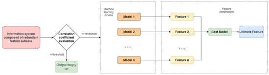
Figure 2. Feature construction flowchart.

In this study, model performance is assessed by employing goodness of fit ($R^2$) along with error metrics such as root mean square error ($RMSE$) and mean absolute percent error ($MAPE$). These metrics evaluate both the model’s ability to fit the observed data and its predictive accuracy. The goodness of fit ($R^2$) is calculated as follows:

$$R^2={\displaystyle \frac{{\displaystyle \sum _{i=1}^n{({\stackrel{⌢}{y}}_i-{\overline{y}}_i)}^2}}{{\displaystyle \sum _{i=1}^n{(y_i-{\overline{y}}_i)}^2}}}$$

(5)

$R^2$ is often used to evaluate the degree of fit of sample data in the model.

Root mean square error reflects the deviation between predicted values and true values. It strengthens the influence of large errors in the indicator, thereby making the sensitivity of the indicator higher. The formula is as follows:

$$RSME=\sqrt{{\displaystyle \frac{1}{n}}{\displaystyle \sum _{i=1}^n{(y_i-{\stackrel{⌢}{y}}_i)}^2}}$$

(6)

The mean absolute percent error ($MAPE$) is a commonly used metric in forecasting and prediction analysis. The $MAPE$ is calculated using the following formula:

$$MAPE={\displaystyle \frac{1}{n}}{\displaystyle \sum _{i=1}^n\left|\frac{y_i-{\stackrel{⌢}{y}}_i}{y_i}\right|}\times 100$$

(7)

3.6. The Overall Algorithm of Feature Engineering

Then, we integrate the first two algorithms to design a new feature engineering algorithm. The algorithm is shown in Algorithm 4.

Algorithm 4. Enhanced feature engineering model (EFEM)

Input: An information system Output: $R^2$, $RMSE$ and $MAPE$ 1. Using the DSA–mRMR algorithm, the feature subset $S$ and its redundant feature subset $S^{\prime }$ are obtained. 2. Evaluate whether the correlation coefficient $\gamma$ of the redundant feature subset is greater than the threshold. If the correlation coefficient $\gamma \ge threshold$, proceed next step; otherwise, jump to step 5. 3. Input the redundant feature subset $S^{\prime }$ as an information system to algorithm RFA, generating a new feature $\tilde{s}$. 4. Merge the feature subset $S$ selected by the DSA–mRMR with the feature constructed in Step 3 to form a new feature subset $S*$. 5. Select the best machine learning model from algorithm RFA to train the extracted feature subset $S*$. 6. Output the results of evaluation indicators, including $R^2$, RMSE and MAPE.

The enhanced feature engineering model (EFEM) is a machine learning pipeline that combines feature selection and feature construction to improve predictive model performance. The algorithm first employs the DSA–mRMR method to filter out a highly relevant, low-redundancy feature subset $S$ and a redundant subset $S^{\prime }$. It then checks the correlation coefficient $\gamma$ of the redundant features—if it exceeds a threshold, the RFA algorithm constructs new features from the redundant subset and merges them with the originally selected features. Finally, the optimal machine learning model is selected for training, and evaluation metrics ($R^2,RMSE,MAPE$) are output. The EFEM’s uniqueness lies in dynamically leveraging redundant information to generate new features, reducing dimensionality while enhancing model expressiveness, making it suitable for high-dimensional regression tasks.

The EFEM model employs a symmetrical dual strategy. A symmetrical decomposition of the feature space is first performed. The DSA–mRMR method is used to precisely select an optimal, highly relevant feature subset, while the remaining features are concurrently identified as a redundant subset. Instead of simply discarding this redundant information, a second symmetrical process is employed: a new synthetic feature is created by the RFA algorithm, which aggregates the seemingly useless features. This new feature serves as a symmetrical complement to the initially selected optimal subset.

The computational complexity of the EFEM is determined by the integration of its feature selection, redundancy handling, and model training phases. Therefore, the overall complexity is dominated by the DSA–mRMR and RFA steps.

4. Experimental Analysis

This section systematically evaluates the regression performance of the enhanced feature engineering model (EFEM) on nine standard UCI datasets [47] to comprehensively validate the model’s effectiveness. In the RFA algorithm, the correlation threshold is set to 0.7. The algorithm employs the following four base models: Bayesian linear regression, random forest regression, CatBoost, and support vector machine. To avoid information leakage, the RFA composite features are constructed within each cross-validation fold using only the training subset. The validation/test folds are strictly excluded from this process, ensuring that the performance estimates remain unbiased. Through comparative analysis, CatBoost is identified as the top-performing algorithm and is consequently selected as the final training model in the framework. The selected features are retrained using CatBoost, with its performance evaluated through 10-fold cross-validation. This process ultimately identifies the optimal feature set for model construction. These parameters undergo extensive validation and tuning to ensure model interpretability while maintaining a stable performance across diverse datasets.

Through multidimensional metrics, the study compares and analyzes the EFEM’s prediction accuracy and feature selection capabilities, and the evaluation metrics include the root mean square error ($RMSE$), mean absolute percentage error ($MAPE$), and goodness-of-fit ($R^2$).

All experiments in this study were conducted on a high-performance computing cluster equipped with an Intel Xeon (R) Platinum 8352 V 32-core processor and 60 GB of RAM. The implementation utilized Python 3.8 within the Anaconda 2021.05 distribution environment, with core dependencies on machine learning libraries, including scikit-learn 1.0.2 and CatBoost 1.0.6, for algorithm development. To ensure reproducibility, results were aggregated over 10 independent trials, with final metrics derived from the arithmetic mean.

4.1. Algorithm Comparison

In order to better evaluate the effectiveness of the EFEM, five similar feature engineering algorithms are selected for comparison. These five algorithms are as follows:

Guo et al. (2020) proposed an Improved Whale Optimization Algorithm for Feature Selection (IWOA-FS) that enhances feature selection performance through dynamic-inertia weights and elite opposition-based learning strategies [48].

Ren et al. (2023) developed a Hybrid High-Dimensional Multi-Target Sparrow Search Algorithm (HDMT-SSA) framework that integrates tent chaotic mapping and Lévy flight strategies to optimize feature selection in high-dimensional data [49].

Aghelpour et al. (2021) integrated the Hybrid Dragonfly Algorithm (HDA-ADP) into an artificial neural network (ANN) framework, developing a novel hybrid model for agricultural drought forecasting [50].

Rostami et al. (2020) proposed a Multi-Objective Particle Swarm Optimization algorithm with Node Centrality (MOPSO-NC) to select biologically significant genetic features using node centrality analysis [51].

Wang et al. (2022) developed the SWDE-FS algorithm, a self-adaptive weighted differential evolution approach that reduces computational complexity to $O(n\log n)$ for large-scale feature selection through an efficient grouped mutation strategy [52].

Next, we further examine the experimental parameters. First, to discretize the target variable, we employ K-means clustering for binning, converting continuous targets into categorical bins, which enables effective F-statistic calculation.

This study employs the DSA–mRMR for feature selection, with the following parameter settings: dolphin population size $N=50$, mutation probability $p_{mut}=0.05$, maximum iterations $T=50$, and convergence threshold $\epsilon \le {10}^{-5}$. The fitness function evaluates feature subsets using the performance metric of a random forest model via 10-fold cross-validation. The critical parameters $\alpha$ and $\beta$ are configured depending on the dataset, with detailed procedures provided in Section 4.5.

As shown in Table 2, the experiments use multiple datasets from the UCI Machine Learning Repository. These datasets vary significantly in size (1059–53,500 samples) and complexity (28–529 features), providing a comprehensive test bench for evaluating the scalability and robustness of the EFEM.

Table 2. Detailed description of the datasets.

ID	DataSet	Abbreviation	Instance	Feature	Source
1	Energydata	ED	19,735	28	UCI
2	WEC_Perth_49	WECP	36,043	149	UCI
3	ValidationData	VD	1111	529	UCI
4	ProcessedDJI	PDJI	1984	82	UCI
5	CommViolPredUnnormalizedData	CVPUD	2214	145	UCI
6	Default_features_1059_tracks	DFT	1059	70	UCI
7	Slice_localization_data	SLD	53,500	386	UCI
8	Superconductivty	SD	21,263	82	UCI
9	UJIndoorLoc-trainingData	UJILD	19,937	529	UCI

The bold values in Table 3 indicate the minimum number of feature selections for each set of experiments. The results show that, except for HDA-ADP, which is superior on the PDJI and DFT datasets, the EFEM selects the least features in all other cases, and has a significant advantage in the average number of feature selections, while HDMT-SSA performs relatively weakest.

Table 3. Number of selected features.

Dataset	IWOA-FS	HDMT-SSA	HDA-ADP	MOPSO-NC	SWDE-FS	EFEM
ED	7	8	4	5	5	3
WECP	52	68	74	79	72	34
VD	187	247	279	263	250	101
PDJI	29	24	19	30	23	26
CVPUD	57	78	76	72	77	38
DFT	31	23	17	23	25	19
SLD	198	196	202	217	196	109
SD	33	35	24	25	24	13
UJILD	189	275	245	268	275	88
Average	87.00	106.00	104.44	109.11	105.22	47.89

Note: The bold value indicates the best performance.

In Table 4, we define the feature reduction rate, and the reduction rate is calculated as follows:

$$reduction=(1-{\displaystyle \frac{\left|S\right|}{\left|A\right|}})\ast 100\%$$

(8)

Table 4. Comparison of feature reduction rates.

Dataset	IWOA-FS	HDMT-SSA	HDA-ADP	MOPSO-NC	SWDE-FS	EFEM
ED	71.43%	67.86%	82.14%	78.57%	78.57%	85.71%
WECP	64.19%	53.38%	49.32%	45.95%	50.68%	76.35%
VD	64.46%	53.12%	47.07%	50.09%	52.55%	80.72%
PDJI	63.41%	69.51%	75.61%	62.20%	70.73%	67.07%
CVPUD	60.00%	45.52%	46.90%	49.66%	46.21%	73.10%
DFT	54.29%	65.71%	74.29%	65.71%	62.86%	71.43%
SLD	48.45%	48.96%	47.41%	43.52%	48.96%	71.50%
SD	58.54%	56.10%	69.51%	68.29%	69.51%	82.93%
UJILD	64.08%	47.83%	53.50%	49.15%	47.83%	83.18%
Average	60.98%	56.44%	60.64%	57.02%	58.66%	76.89%

Note: The bold value indicates the best performance.

The bold data in Table 4 indicates the row with the best reduction rate. Comparative analysis shows that the EFEM algorithm exhibits the best reduction performance in most cases. Specifically, with the exception of the HDA-ADP algorithm, which performs slightly better on the PDJI and DFT datasets, the EFEM algorithm achieves the best reduction results in all other comparison experiments. Statistical results show that the EFEM algorithm achieves an average reduction rate of 76.89%, significantly outperforming the other compared algorithms. A comprehensive evaluation shows that the EFEM algorithm achieves the best overall performance, while the HDFT-SSA performs relatively poorly.

As shown in Table 5, the numbers in brackets represent the ranking of the goodness of fit ($R^2$) of each algorithm. The analysis results show that the EFEM algorithm ranks first on six of the nine datasets and ranks third on the remaining three datasets, with an average ranking of 1.67, which is significantly better than other comparison algorithms. In addition, the average goodness of fit of the EFEM algorithm reaches 0.9263, further verifying its excellent performance in model fitting. In contrast, the SWDE-FS algorithm performs poorly.

Table 5. Algorithm goodness-of-fit ($R^2$) comparison and ranking.

Dataset	RAW	IWOA-FS	HDMT-SSA	HDA-ADP	MOPSO-NC	SWDE-FS	EFEM
ED	1	0.998 (6)	0.9998 (3)	0.9998 (3)	0.9998 (3)	0.9998 (3)	0.9998 (3)
WECP	0.9974	0.9932 (4.5)	0.9934 (2)	0.9933 (3)	0.9931 (6)	0.9932 (4.5)	0.9972 (1)
VD	0.8816	0.6994 (6)	0.8397 (3)	0.8412 (2)	0.8048 (4)	0.7124 (5)	0.863 (1)
PDJI	0.7813	0.7726 (1)	0.7668 (4)	0.7693 (2)	0.6629 (6)	0.6662 (5)	0.7658 (3)
CVPUD	0.955	0.7178 (5)	0.6979 (6)	0.9413 (2)	0.7511 (3)	0.7454 (4)	0.9321 (1)
DFT	0.7756	0.7208 (3)	0.7164 (5)	0.7142 (6)	0.7267 (2)	0.7206 (4)	0.8569 (1)
SLD	0.9915	0.949 (2)	0.9474 (3)	0.945 (4)	0.9445 (5)	0.9432 (6)	0.997 (1)
SD	0.9217	0.8751 (5)	0.8702 (6)	0.8765 (4)	0.8874 (2)	0.8767 (3)	0.9256 (1)
UJILD	0.9999	0.9682 (6)	0.998 (4)	0.9997 (1.5)	0.9997 (1.5)	0.9861 (5)	0.9996 (3)
Average	0.9227	0.8549 (5)	0.8700 (3)	0.8978 (2)	0.8633 (4)	0.8493 (6)	0.9263 (1)

Note: The bold value indicates the best performance.

As shown in Table 6, the numbers in parentheses indicate the root mean square error ($RMSE$) ranking of each algorithm. The experimental results show that the EFEM algorithm performs exceptionally well on the nine datasets, ranking first on five, second on two, third on one, and fourth on one. Its overall ranking significantly outperforms the other compared algorithms. In contrast, the SWDE-FS algorithm performs poorly overall.

Table 6. Algorithm root mean square error ($RMSE$) comparison and ranking.

Dataset	RAW	IWOA-FS	HDMT-SSA	HDA-ADP	MOPSO-NC	SWDE-FS	EFEM
ED	0.0767	0.2203 (5)	0.21 (1)	0.2232 (6)	0.2126 (3)	0.2121 (2)	0.2168 (4)
WECP	6296.08	10,114.9622 (5)	9952.0156 (2)	10,048.0822 (3)	10,200.03 (6)	10,108.1293 (4)	6450.2137 (1)
VD	170,092.4411	272,350.3021 (6)	198,663.4525 (3)	197,137.7314 (2)	218,482.4 (4)	266,203.1996 (5)	180,742.3109 (1)
PDJI	0.4715	0.4807 (1)	0.8266 (6)	0.4861 (2)	0.5875 (5)	0.5855 (4)	0.4877 (3)
CVPUD	519.0804	1409.5336 (5)	1460.5124 (6)	617.5007 (1)	1324.887 (3)	1339.1683 (4)	670.6632 (2)
DFT	23.5548	26.3888 (4)	26.5613 (5)	26.7005 (6)	26.0769 (2)	26.3060 (3)	18.7478 (1)
SLD	2.0597	5.0445 (2)	5.1216 (3)	5.2383 (4)	5.264 (5)	5.3258 (6)	1.2119 (1)
SD	9.5736	12.0863 (6)	12.0021 (3)	12.0231 (5)	11.9754 (2)	12.0116 (4)	9.3235 (1)
UJILD	4575.9941	24,735.8124 (4)	24,680.8435 (3)	9414.0578 (6)	28,421.17 (5)	65,147.41 (1)	10,312.0809 (2)
Average	20,168.8147	34,294.9812 (5)	26,089.0606 (3)	24,140.2270 (2)	28,719.1782 (4)	38,093.5942 (6)	22,022.8063 (1)

Note: The bold value indicates the best performance.

As shown in Table 7, the numbers in brackets represent the ranking of the mean absolute percentage error ($MAPE$) of each algorithm. The analysis results show that the EFEM algorithm once again performs best, with an average $MAPE$ of 1.2023. The $MAPE$ on the SLD dataset is only 0.0209, which is 77.5% lower than the 0.093 of SWDE-FS, and it is 5.5687 on the SD dataset, which is 36.5% lower than the 8.7652 of SWDE-FS, demonstrating its excellent reliability in controlling relative prediction errors. In contrast, the MOPSO-NC algorithm performs poorly.

Table 7. Algorithm mean absolute percentage error (MAPE) comparison and ranking.

Dataset	RAW	IWOA-FS	HDMT-SSA	HDA-ADP	MOPSO-NC	SWDE-FS	EFEM
ED	0.0169	0.0312 (1)	0.0313 (2)	0.0337 (6)	0.0315 (3)	0.0317 (4)	0.0325 (5)
WECP	0.0009	0.0020 (3.5)	0.0099 (6)	0.0020 (3.5)	0.0020 (3.5)	0.0020 (3.5)	0.0009 (1)
VD	0.0001	0.0001 (3.5)	0.0001 (3.5)	0.0001 (3.5)	0.0001 (3.5)	0.0001 (3.5)	0.0001 (3.5)
PDJI	3.04978 × 1012	3.247 × 1012 (3)	4.052 × 1012 (4)	2.256 × 1012 (1)	5.13 × 1012 (6)	4.395 × 1012 (5)	2.673 × 1012 (2)
CVPUD	0.0316	0.2366 (6)	0.2347 (5)	0.0603 (1)	0.2198 (3)	0.2241 (4)	0.0654 (2)
DFT	3.9544	4.98 (4)	5.1666 (6)	4.9009 (3)	4.9874 (5)	4.6674 (2)	2.4589 (1)
SLD	0.0375	0.0902 (2)	0.0903 (4)	0.0914 (5)	0.0902 (2)	0.093 (6)	0.0209 (1)
SD	6.4343	8.7032 (4)	8.7154 (5)	8.4673 (2)	8.4825 (3)	8.7652 (6)	5.5687 (1)
UJILD	0	0 (3.5)	0 (3.5)	0 (3.5)	0 (3.5)	0 (3.5)	0 (3.5)
Average		1.9211 (3)	2.0334 (4)	1.7568 (2)	2.1048 (6)	2.0198 (5)	1.2023 (1)

Note: The bold value indicates the best performance.

4.2. Statistical Analysis

To rigorously compare algorithm performance, we conducted Wilcoxon signed-rank tests under a paired experimental design to assess statistical significance. The results of the Wilcoxon signed-rank tests between the EFEM algorithm and other comparative algorithms are presented in Table 8. With a significance level of $\alpha =0.05$, $p<\alpha$ indicates statistically significant differences between the algorithms.

Table 8. Wilcoxon paired test results for algorithms’ comparison.

Paired Variables	Median ± Standard Deviation			z	df	p	Cohen’s d
	Paired 1	Paired 2	Paired Difference (Paired 1 − Paired 2)
EFEM vs. IWOA-FS	0.932 ± 0.083	0.875 ± 0.127	0.048 ± 0.08	2.31	8	0.01953	0.668
EFEM vs. HDMT-SSA	0.932 ± 0.083	0.87 ± 0.122	0.023 ± 0.081	2.521	8	0.01172	0.543
EFEM vs. HDA-ADP	0.932 ± 0.083	0.931 ± 0.104	0.004 ± 0.047	1.96	8	0.04995	0.317
EFEM vs. MOPSO-NC	0.932 ± 0.083	0.887 ± 0.13	0.052 ± 0.064	2.38	8	0.01729	0.579
EFEM vs. SWDE-FS	0.932 ± 0.083	0.877 ± 0.138	0.054 ± 0.069	2.521	8	0.01172	0.681

Table 8 displays the model test results (median, p-value, degrees of freedom, significance value, and effect size), with an analysis of the statistical significance of p-values for each paired sample group. If it is significant ($p<0.05$), the null hypothesis is rejected, indicating that there are differences between each group of paired samples. Otherwise, it means that there is no significant difference between each group of paired samples. Cohen’s d value represents the difference effect size. A value less than 0.2 indicates that the difference is very small; a value within [0.2, 0.5) indicates that the difference is small; a value within [0.5, 0.8) indicates that the difference is medium; and a value greater than 0.8 indicates that the difference is very large.

Table 8 presents the results of paired comparisons involving the variable EFEM across five pairings, analyzed using non-parametric tests (indicated by Z-scores). All pairings exhibited statistically significant differences, with p-values ranging from 0.01172 to 0.04995. The EFEM pairing with SWDE-FS exhibited the largest effect size (Cohen’s d = 0.681), along with the highest median difference (0.054 ± 0.069) among all pairings.

In contrast, the EFEM pairing with HDA-ADP showed the smallest median difference (0.004 ± 0.047) and effect size (d = 0.317), though they were still statistically significant.

The overall performance of the EFEM algorithm is robust, it can consistently detect statistically significant differences, and it shows a strong discrimination ability in some pairings. Therefore, the performance of the EFEM algorithm is good and worthy of further promotion.

4.3. Algorithm Convergence and Runtime

To comprehensively evaluate the convergence, efficiency, and robustness of the proposed DSA–mRMR algorithm, convergence experiments were conducted on four different datasets. Figure 3 shows the relationship between the number of algorithm iterations and the number of selected features for these datasets. As shown, the number of selected features decreases steadily with increasing iterations and eventually stabilizes. This demonstrates that the DSA–mRMR algorithm, through its iterative optimization mechanism, gradually eliminates redundant and irrelevant features, thereby effectively compressing the feature dimension.

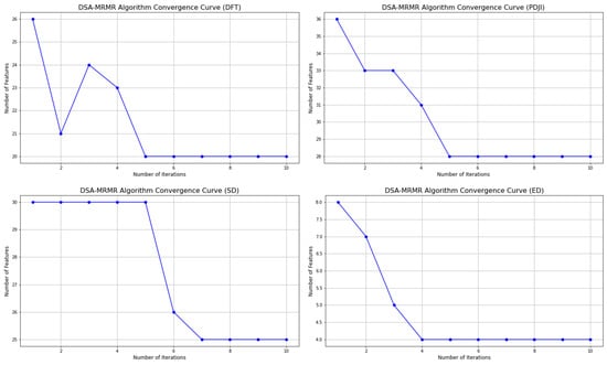
Figure 3. DSA–mRMR algorithm convergence curve.

The plateau of the curve indicates successful convergence of the algorithm. This not only demonstrates that the DSA–mRMR algorithm can find an optimal or suboptimal feature subset, but also demonstrates the effectiveness and reliability of its optimization process. The number of features stabilizes after a relatively small number of iterations, indicating that the algorithm can efficiently complete the feature selection task, avoiding unnecessary redundant computations and significantly improving overall efficiency. The stable convergence curve indicates that after reaching the optimal solution, the algorithm’s search process does not experience drastic fluctuations or performance degradation, demonstrating its high robustness in complex data environments.

The computational efficiency of the EFEM algorithm was compared with other algorithms on four datasets. The results showed that EFEM’s runtime exhibited dataset-dependent characteristics. Table 9 shows that on the VD and CVPUD datasets, the algorithm achieved the shortest runtime, demonstrating a clear advantage in computational efficiency. However, on the DFT and PDJI datasets, its runtime ranked relatively low, second and fourth, respectively.

Table 9. Comparison and ranking of algorithm running time (unit: seconds).

Dataset	IWOA-FS	HDMT-SSA	HDA-ADP	MOPSO-NC	SWDE-FS	EFEM
DFT	1149.98 (4)	1019.76 (3)	1287.56 (5)	1319.82 (6)	890.34 (1)	1017.76 (2)
VD	4.98 (4)	3.19 (2)	5.76 (5)	7.1 (6)	4.56 (3)	2.27 (1)
PDJI	2567.83 (3)	2141.09 (1)	8987.48 (6)	3000.76 (5)	2382.37 (2)	2863.43 (4)
CVPUD	57.21 (6)	14.94 (2)	20.12 (3)	21.09 (4)	36.37 (5)	13.81 (1)
Average time	945 (3)	794.745 (1)	2575.23 (6)	1087.1925 (5)	828.41 (2)	974.318 (4)

Note: The bold value indicates the best performance.

Overall, although the EFEM ranked fourth in average runtime, it generally ranked high in predictive performance (as shown in Table 5, Table 6 and Table 7). This demonstrates that the EFEM strikes a balance between computational efficiency and model performance, providing a reliable solution for applications requiring a high accuracy.

4.4. Ablation Study

A series of ablation experiments were conducted to evaluate the effectiveness of the EFEM model and the contributions of its key components. The experimental results are shown in Table 10. The goodness of fit of the following four different model configurations was evaluated: the EFEM model (the full model), the RFA model (using only redundant feature aggregation, without DSA–mRMR, and using all dataset features), the DSA–mRMR model (using only DSA–mRMR feature selection, without redundant feature aggregation), and the DSA model (the baseline model, without DSA–mRMR and redundant feature aggregation). The experimental results showed that on most datasets, the model goodness of fit exhibited a consistent ranking: DSA < DSA–mRMR < RFA < EFEM. This result strongly demonstrates the effectiveness of the DSA–mRMR feature selection and the redundant feature aggregation (RFA) module. The DSA–mRMR module significantly improved model performance by selecting the most representative features. The redundant feature aggregation (RFA) module further enhanced the model’s fit by effectively utilizing redundant information.

Table 10. Results of ablation study on the different algorithm ($R^2$).

Dataset	DSA	DSA–mRMR	RFA	AE	SSL	EFEM
ED	0.9521 (6)	0.9816 (4)	0.9698 (5)	0.9951 (2)	0.9901 (3)	0.9998 (1)
WECP	0.9327 (6)	0.9656 (5)	0.9671 (4)	0.9785 (3)	0.9904 (2)	0.9972 (1)
VD	0.8115 (6)	0.8471 (4)	0.8237 (5)	0.8527 (3)	0.859 (2)	0.863 (1)
PDJI	0.6911 (6)	0.7518 (4)	0.7358 (5)	0.7602 (3)	0.7675 (1)	0.7658 (2)
CVPUD	0.8845 (6)	0.9109 (4)	0.9069 (5)	0.9189 (3)	0.9287 (2)	0.9321 (1)
DFT	0.7961 (6)	0.8382 (4)	0.8195 (5)	0.8414 (3)	0.8537 (2)	0.8569 (1)
SLD	0.9566 (6)	0.9821 (4)	0.9752 (5)	0.9863 (3)	0.9891 (2)	0.997 (1)
SD	0.8764 (6)	0.9024 (4)	0.8956 (5)	0.9145 (3)	0.9214 (2)	0.9256 (1)
UJILD	0.9435 (6)	0.9877 (4)	0.9702 (5)	0.9927 (3)	0.9986 (2)	0.9996 (1)
Average	0.8716 (6)	0.9075 (4)	0.8960 (5)	0.9156 (3)	0.9221 (2)	0.9263 (1)

A comparison of the EFEM algorithm with two independent deep learning-based feature extraction methods and self-supervised learning feature extraction was also performed to verify the effectiveness of our hybrid strategy. As shown in Table 10, they achieved an average ranking of third and second, respectively, demonstrating the powerful capabilities of deep learning for feature extraction, especially when working with complex datasets.

As a complete model integrating all optimized components, the EFEM exhibited the best goodness of fit among all configurations, validating the superiority of its design.

4.5. Parameter Sensitivity Analysis

To determine the optimal number of clusters (K) for discretizing the target variable, the elbow method was employed. As shown in Figure 4, our analysis of the PDJI, CVPUD, DFT, and VD datasets reveals that the elbow of the curves consistently appeared at K = 2. This indicates that discretizing the target variables of these datasets into two categories is the most effective choice for reducing intra-cluster error and provides a solid theoretical foundation for our algorithm.

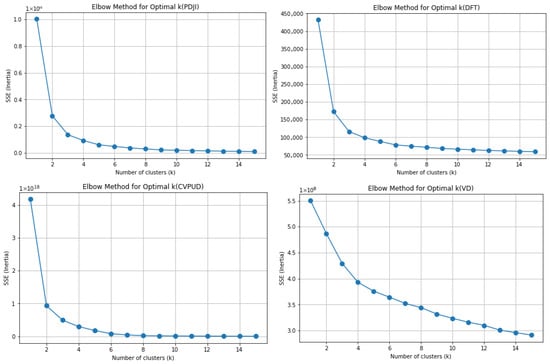
Figure 4. Elbow method for optimal k.

While the elbow rule provides a theoretical basis for choosing K = 2, sensitivity analysis was further conducted on the choice of K to verify the robustness of our algorithm. This analysis was performed on four datasets. As shown in Figure 5, while changes in K slightly affect model performance, the curves for metrics such as $R^2$, $RMSE$, and $MAPE$ all fluctuate within a narrow range, indicating that model performance remains stable and high. This strongly demonstrates that our algorithm can reliably identify core feature subsets under different discretization methods, ultimately achieving a robust predictive performance.

Figure 5. Performance metrics sensitivity analysis to K value.

Analysis on the DFT dataset, as a representative subplot in Figure 5, visually confirms this robustness. The curves for $R^2$, $RMSE$, and $MAPE$ show that while performance varies slightly as K increases, the overall trend remains strong. Specifically, the $R^2$ value remains consistently high, while the $RMSE$ and $MAPE$ values stay low across different K values. This further validates that the algorithm’s performance is not overly sensitive to the choice of K and can maintain stability in a variety of scenarios.

To evaluate the impact of parameters $\alpha$ (controlling the trade-off between feature relevance and redundancy) and $\beta$ (adjusting the penalty term for dimensionality reduction) on model performance, this study conducted a grid search to test $R^2$ values under different parameter combinations, visualized through 3D surface plots (as shown in Figure 6). The analysis revealed that the model achieved an optimal performance ($R^2$ > 0.92) when $\alpha$ ranged between 0.4 and 0.6 and $\beta$ ≤ 0.3.

Figure 6. Three-dimensional surface plots.

The 3D surface plot shown in subfigure (PDJI 3D Surface Plot) clearly illustrates the results of a parameter sensitivity analysis of the EFEM on the PDJI dataset. The horizontal axis ($\alpha$) represents the balance coefficient between feature relevance and redundancy, the vertical axis ($\beta$) represents the regularization strength during dimensionality reduction, and this axis quantifies the model performance index (ranging from 0.1 to 0.81). The results indicate that surface fluctuations are primarily due to the following mechanisms: nonlinear coupling between parameters, with the model achieving an optimal performance when $\alpha \in \left[0.2,0.4\right]$ and $\beta \in \left[0.6,0.8\right]$, and performance degradation caused by suboptimal parameter combinations (minimum 0.7).

Under these conditions, the feature subset effectively retains highly informative features while suppressing redundancy. The surface plot exhibits a distinct peak at $\alpha$ = 0.5 and $\beta$ = 0.2, demonstrating the synergistic effect of the mRMR criterion and the dimensionality reduction penalty. Conversely, when $\alpha$ > 0.7 or $\beta$ > 0.5, $R^2$ sharply declines, indicating that overemphasizing relevance or dimensionality reduction leads to information loss. These results confirm the sensitivity of parameter selection and provide quantitative guidance for parameter tuning in practical applications.

A sensitivity analysis was also conducted on the correlation threshold $\gamma$, a key parameter of the RFA algorithm. Although the thresholds and model selections might appear empirical, their robustness was examined through sensitivity analyses. Specifically, correlation thresholds of 0.6, 0.7, and 0.8 were compared, and the BLR and RF models were used for evaluating the performance. As shown in Table 11, the results showed that 0.7 provided a good balance between redundancy reduction and information retention, and CatBoost consistently outperformed other models in terms of accuracy and stability. These findings confirm that our design choices are both theoretically sound and empirically justified.

Table 11. Comparison of RFA thresholds under different models.

$\mathit{\gamma }$	0.6		0.7		0.8		0.7
Dataset	BLR	RF	BLR	RF	BLR	RF	CatBoost
ED	0.9107	0.9395	0.9209	0.9439	0.9054	0.9239	0.9618
WECP	0.8876	0.9401	0.9165	0.9488	0.8947	0.9498	0.9521
VD	0.779	0.8001	0.7809	0.8131	0.7612	0.7823	0.8176
PDJI	0.6478	0.6976	0.6598	0.7002	0.6295	0.6809	0.7189

4.6. Robustness Analysis

To comprehensively evaluate the robustness of an algorithm, the following steps are typically required: normal condition testing, noise testing, abnormal condition testing, and stress testing. Among these experiments, noise testing focuses on examining the algorithm’s robustness to noise. Specifically, noise is introduced into the dataset and the algorithm is run multiple times on it to assess its noise resistance. Four datasets were selected from Table 2 for this experiment, with 25% of the real-valued data randomly selected from each dataset for noise injection testing.

In the experiments conducted on the four original datasets, the EFEM significantly outperformed the other algorithms. On the noisy datasets, it was readily apparent that these values degraded to varying degrees compared to the data in Table 5, Table 6 and Table 7. A comparative analysis of the six algorithms was conducted, with detailed experimental results listed in Table 12, Table 13 and Table 14. However, the EFEM’s overall performance remained superior. The noise experiments further demonstrate the EFEM’s superior performance.

Table 12. Algorithm goodness-of-fit ($R^2$) comparison and ranking on noisy datasets.

Dataset	IWOA-FS	HDMT-SSA	HDA-ADP	MOPSO-NC	SWDE-FS	EFEM
WECP	0.9785 (4)	0.9859 (2)	0.9841 (3)	0.9527 (6)	0.9672 (5)	0.9933 (1)
VD	0.5892 (6)	0.7988 (2)	0.7230 (3)	0.6558 (4)	0.6014 (5)	0.8006 (1)
DFT	0.7249 (3)	0.6325 (5)	0.5891 (6)	0.7513 (2)	0.6987 (4)	0.7764 (1)
CVPUD	0.6419 (5)	0.5537 (6)	0.7891 (2)	0.7258 (4)	0.7322 (3)	0.7986 (1)
Average	0.7336 (6)	0.7427 (5)	0.7713 (4)	0.7714 (3)	0.7499 (2)	0.8422 (1)

Note: The bold value indicates the best performance.

Table 13. Algorithm root mean square error ($RMSE$) comparison and ranking on noisy datasets.

Dataset	IWOA-FS	HDMT-SSA	HDA-ADP	MOPSO-NC	SWDE-FS	EFEM
WECP	20,172.8539 (3)	23,821.3829 (5)	26,865.1093 (6)	18,920.9453 (2)	23,018.8279 (4)	10,045.2812 (1)
VD	386,459.2094 (6)	240,875.0185 (2)	246,910.7593 (3)	309,285.7915 (4)	372,391.8407 (5)	220,817 (1)
DFT	40.6071 (4)	46.6051 (3)	58.2379 (6)	38.0857 (2)	45.9170 (5)	29.6055 (1)
CVPUD	2891.1892 (5)	3403.3978 (6)	967.9319 (1)	2098.3655 (3)	2181.5067 (4)	1187.0132 (2)
Average	102,390.9649 (6)	67,036.6011 (2)	68,700.5096 (3)	82,585.797 (4)	99,409.5231 (5)	58,019.725 (1)

Note: The bold value indicates the best performance.

Table 14. Algorithm mean absolute percentage error ($MAPE$) comparison and ranking on noisy data.

Dataset	IWOA-FS	HDMT-SSA	HDA-ADP	MOPSO-NC	SWDE-FS	EFEM
WECP	0.0040 (2)	0.0258 (6)	0.0090 (3)	0.0180 (5)	0.0120 (4)	0.002 (1)
VD	0.0001 (3.5)	0.0001 (3.5)	0.0001 (3.5)	0.0001 (3.5)	0.0001 (3.5)	0.0001 (3.5)
DFT	12.4891 (5)	15.8349 (6)	12.1374 (3)	12.5109 (4)	9.0215 (2)	5.436 (1)
CVPUD	0.8961 (6)	0.8752 (5)	0.1970 (1)	0.5898 (3)	0.6544 (4)	0.1588 (2)
Average	3.3473 (5)	4.1838 (6)	3.0858 (3)	3.279475 (4)	2.422 (2)	1.3992 (1)

Note: The bold value indicates the best performance.

4.7. Application on Order Demand Prediction

To further evaluate the applicability of the EFEM model in real-world, high-dimensional forecasting scenarios, the algorithm was applied to product demand forecasting. The algorithm used historical data [53] (2015–2018) from a Chinese manufacturing company to forecast product demand, focusing on the first quarter of 2019. The experimental dataset contained 597,694 samples. The original dataset contained 8 features, which were expanded to 18 features after feature reconstruction, reflecting product pricing and demand in different sales regions.

Four machine learning algorithms, namely random forest (RF), Bayesian linear regression (BLR), Support Vector Regression (SVR), and CatBoost, were selected to constitute the foundational base models for the EFEM ensemble framework. Optimized feature selection was performed by the EFEM, ultimately identifying a refined subset of the following five significant features: season, holiday type, holiday, promotion type, and promotion activity. As shown in Table 15, Table 16 and Table 17, the individual methods were significantly outperformed by the EFEM. In a comparison of the experimental EFEMs, the CatBoost-based ensemble model achieved the highest accuracy ($R^2=0.894$).

Table 15. Model prediction results.

Sales_Region	Item_Code	Jan 2019	Feb 2019	Mar 2019
101	20002	82.55	67.367	55.05
101	20003	181.40	152.09	140.16
101	20006	71.06	50.05	66.04
…	…	…	…	…
105	22066	1273.51	828.63	549.08
105	22072	380.45	225.94	200.52
$R^2=0.894$

Table 16. Comparison of RMSE.

Model	Month		Week		Day
	Training Set	Test Set	Training Set	Test Set	Training Set	Test Set
RF	1172	729	429	291	159	131
BLR	1139	662	386	278	138	120
SVR	1119	569	447	246	134	122
CatBoost	1228	652	427	284	148	121
Fusion	295		91		44

Table 17. Comparison of MAPE.

Model	Month		Week		Day
	Training Set	Test Set	Training Set	Test Set	Training Set	Test Set
RF	1460	1917	753	1206	451	699
BLR	1740	2328	709	1127	346	445
SVR	316	458	215	352	324	408
CatBoost	1772	2370	789	1261	357	457
Fusion	335		247		203

Long Short-Term Memory (LSTM) networks are an improvement upon Recurrent Neural Networks (RNNs). LSTM demonstrates a good performance in long-term memory tasks, and as a result, it is widely applied in nonlinear time series prediction. In this section, products are classified based on regions, and products within the same region are extracted and demand is aggregated on a monthly basis. Data is organized with products as rows and time as columns. Finally, LSTM is employed for single-step forecasting.

After adjusting the learning rate and iterations, the final forecast results indicate a significant presence of negative values, which are treated as zeros. Due to these zero values, $MAPE$ is not suitable as a model evaluation metric. Therefore, only $RMSE$ and $R^2$ are computed to gauge the predictive accuracy of the model. The predicted results are shown in Table 18. The results of the aforementioned forecast highlight significant errors, with both and RMSE indicating a poor predictive performance of the model.

Table 18. LSTM prediction results.

Item_Code	Forecast Results
20001	0
20002	32.035
20003	354.009
…	…
22081	682.225
22084	2.857
$R^2=0.239$	$RMSE$ = 505.143

We ultimately concluded that the EFEM provides the most effective and accurate forecasts for enterprise production planning.

5. Conclusions

This study proposes an enhanced feature engineering model (EFEM) that effectively addresses the key challenges in high-dimensional regression tasks, including local optimal convergence and inefficient redundant feature processing. The model achieves this by integrating the Dolphin Swarm Algorithm (DSA) with the Maximum Relevance–Minimum Redundancy (mRMR) method. EFEM contains the following two major innovations: (1) the DSA–mRMR algorithm, which uses a dynamic fitness function to optimize feature selection and balance feature relevance and redundancy, and (2) a developed feature construction algorithm that employs an ensemble learning strategy to fuse redundant features and generate more discriminative synthetic features. Finally, the model combines the optimal feature subset with the synthetic features to further improve prediction performance.

Experiments conducted on nine UCI regression datasets showed that the EFEM significantly outperformed baseline methods in both prediction accuracy and computational efficiency, achieving average performance metrics of $R^2$ = 0.9263, $RMSE$ = 22,022.81, and $MAPE$ = 1.2023. The statistical significance of this performance improvement was confirmed by a Wilcoxon signed-rank test. Furthermore, the model selected an average of only 47.89 features (achieving a dimensionality reduction rate of 76.89%), which substantially improved computational efficiency while maintaining accuracy. A comprehensive analysis of parameter sensitivity, robustness, convergence, and ablation experiments demonstrated the EFEM’s exceptional stability and reliability in complex data environments. The model’s successful application in a real-world product demand forecasting task further validated its practical value in industrial scenarios.

Future research will concentrate on two main directions. On one hand, we will focus on optimizing the algorithm’s architecture by integrating adaptive learning with new intelligent algorithms to further improve model efficiency. On the other hand, we will expand its industrial application scenarios, verify its real-time performance in fields such as intelligent manufacturing and financial forecasting, and develop incremental learning functions to promote technological implementation. These works will provide more powerful and practical solutions for high-dimensional data processing.

References

- An, J.; Kim, I.S.; Kim, K.-J.; Park, J.H.; Kang, H.; Kim, H.J.; Kim, Y.S.; Ahn, J.H. Efficacy of automated machine learning models and feature engineering for diagnosis of equivocal appendicitis using clinical and computed tomography findings. Sci. Rep. 2024, 14, 22658. [Google Scholar] [CrossRef] [PubMed]
- Zhao, Y.; Zhang, W.; Yang, T.; Jiang, Y.; Huang, F.; Lim, W.Y.B. STORM: A Spatio-Temporal Factor Model Based on Dual Vector Quantized Variational Autoencoders for Financial Trading. arXiv 2024, arXiv:2412.09468. [Google Scholar] [CrossRef]
- Siemens Senseye. The Transformative Role of Generative AI in Predictive Maintenance [White Paper]; Siemens Digital Industries: Plano, TX, USA, 2024. [Google Scholar]
- Kraev, E.; Koseoglu, B.; Traverso, L.; Topiwalla, M. Shap-Select: Lightweight feature selection using SHAP values and regression. arXiv 2024, arXiv:2410.06815. [Google Scholar] [CrossRef]
- Benítez-Peña, S.; Blanquero, R.; Carrizosa, E.; Ramírez-Cobo, P. Cost-sensitive feature selection for support vector machines. arXiv 2024, arXiv:2401.07627. [Google Scholar] [CrossRef]
- Abhyankar, N.; Shojaee, P.; Reddy, C.K. LLM-FE: Automated feature engineering for tabular data with LLMs as evolutionary optimizers. arXiv 2025, arXiv:2503.14434. [Google Scholar] [CrossRef]
- Wang, K.; Wang, P.; Xu, C. Toward efficient automated feature engineering. arXiv 2022, arXiv:2212.13152. [Google Scholar] [CrossRef]
- Verdonck, T.; Baesens, B.; Oskarsdottir, M.; van den Broucke, S. Special Issue on Advances in Feature Engineering. Mach. Learn. 2021, 113, 3917–3928. [Google Scholar] [CrossRef]
- Duan, Y.; Zhang, G.; Wang, S.; Peng, X.; Ziqi, W.; Mao, J.; Wu, H.; Jiang, X.; Wang, K. CaT-GNN: Enhancing credit card fraud detection via causal temporal graph neural networks. arXiv 2024, arXiv:2402.14708. [Google Scholar] [CrossRef]
- Radford, A.; Kim, J.W.; Hallacy, C. Learning transferable visual models from natural language supervision. In Proceedings of the 38th International Conference on Machine Learning, Virtual, 18–24 July 2021; Volume 139, pp. 8748–8763. [Google Scholar]
- Yu, W.; Liu, Y.; Dillon, T.; Rahayu, W. Edge computing-assisted IIoT framework with an autoencoder for fault detection in manufacturing predictive maintenance. IEEE Trans. Ind. Inform. 2022, 19, 5701–5710. [Google Scholar] [CrossRef]
- da Silva, F.R.; Camacho, R.; Tavares, J.M.R. Federated learning in medical image analysis: A systematic survey. Electronics 2023, 13, 47. [Google Scholar] [CrossRef]
- Rieke, N.; Hancox, J.; Li, W.; Milletarì, F.; Roth, H.R.; Albarqouni, S.; Bakas, S.; Galtier, M.N.; Landman, B.A.; Maier-Hein, K.; et al. The future of digital health with federated learning. NPJ Digit. Med. 2020, 3, 119. [Google Scholar] [CrossRef]
- Achiam, J.; Adler, S.; Agarwal, S.; Ahmad, L.; Akkaya, I.; Aleman, F.L.; Almeida, D.; Altenschmidt, J.; Altman, S.; Anadkat, S.; et al. GPT-4 technical report. arXiv 2023, arXiv:2303.08774v6. [Google Scholar] [CrossRef]
- Yang, H.; Yuan, J.; Li, C.; Zhao, G.; Sun, Z.; Yao, Q.; Bao, B.; Vasilakos, A.V.; Zhang, J. BrainIoT: Brain-like productive services provisioning with federated learning in industrial IoT. IEEE Internet Things J. 2021, 9, 2014–2024. [Google Scholar] [CrossRef]
- Yang, H.; Yu, T.; Liu, W.; Yao, Q.; Meng, D.; Vasilakos, A.V.; Cheriet, M. PAINet: An integrated passive and active intent network for digital twins in automatic driving. IEEE Commun. Mag. 2024, 63, 32–38. [Google Scholar] [CrossRef]
- Yang, H.; Zhao, X.; Yao, Q.; Yu, A.; Zhang, J.; Ji, Y. Accurate fault location using deep neural evolution network in cloud data center interconnection. IEEE Trans. Cloud Comput. 2020, 10, 1402–1412. [Google Scholar] [CrossRef]
- Zhang, C.; Yang, H.; Zhang, C.; Zhang, J.; Yao, Q.; Wang, Z.; Vasilakos, A.V. Federated cross-chain trust training for distributed smart grid in Web 3.0. Appl. Soft Comput. 2025, 180, 113313. [Google Scholar] [CrossRef]
- Yao, Q.; Yang, H.; Li, C.; Bao, B.; Zhang, J.; Cheriet, M. Federated transfer learning framework for heterogeneous edge IoT networks. China Commun. 2023. [Google Scholar] [CrossRef]
- Gulati, A.; Felahatpisheh, A.; Valderrama, C.E. Feature engineering through two-level genetic algorithm. Mach. Learn. Appl. 2025, 21, 100696. [Google Scholar] [CrossRef]
- Song, X.; Zhang, Y.; Gong, D.; Liu, H.; Zhang, W. Surrogate sample-assisted particle swarm optimization for feature selection on high-dimensional data. IEEE Trans. Evol. Comput. 2022, 27, 595–609. [Google Scholar] [CrossRef]
- Ma, W.; Zhou, X.; Zhu, H.; Li, L.; Jiao, L. A two-stage hybrid ant colony optimization for high-dimensional feature selection. Pattern Recognit. 2021, 116, 107933. [Google Scholar] [CrossRef]
- Saheed, Y.K. A binary firefly algorithm based feature selection method on high dimensional intrusion detection data. In Illumination of Artificial Intelligence in Cybersecurity and Forensics; Springer International Publishing: Cham, Switzerland, 2022; pp. 273–288. [Google Scholar]
- Pethe, Y.S.; Gourisaria, M.K.; Singh, P.K.; Das, H. FSBOA: Feature selection using bat optimization algorithm for software fault detection. Discov. Internet Things 2024, 4, 6. [Google Scholar] [CrossRef]
- Arroba, P.; Risco-Martín, J.L.; Zapater, M.; Moya, J.M.; Ayala, J.L. Enhancing regression models for complex systems using evolutionary techniques for feature engineering. arXiv 2024, arXiv:2407.00001. [Google Scholar] [CrossRef]
- Prokhorenkova, L.; Gusev, G.; Vorobev, A.; Dorogush, A.V.; Gulin, A. CatBoost: Unbiased boosting with categorical features. Adv. Neural Inf. Process. Syst. 2018, 31, 6639–6649. [Google Scholar]
- Lim, B.; Arık, S.Ö.; Loeff, N.; Pfister, T. Temporal fusion transformers for interpretable multi-horizon forecasting. Int. J. Forecast. 2021, 37, 1748–1764. [Google Scholar] [CrossRef]
- Khatir, A.; Capozucca, R.; Khatir, S.; Magagnini, E.; Le Thanh, C.; Riahi, M.K. Advancements and emerging trends in integrating machine learning and deep learning for SHM in mechanical and civil engineering: A comprehensive review. J. Braz. Soc. Mech. Sci. Eng. 2025, 47, 419. [Google Scholar] [CrossRef]
- Mansouri, A.; Tiachacht, S.; Ait-Aider, H.; Khatir, S.; Khatir, A.; Cuong-Le, T. A novel Optimization-Based Damage Detection in Beam Systems Using Advanced Algorithms for Joint-Induced Structural Vibrations. J. Vib. Eng. Technol. 2025, 13, 486. [Google Scholar] [CrossRef]
- Khatir, A.; Capozucca, R.; Khatir, S.; Magagnini, E.; Cuong-Le, T. Enhancing damage detection using reptile search algorithm-optimized neural network and frequency response function. J. Vib. Eng. Technol. 2025, 13, 88. [Google Scholar] [CrossRef]
- Khatir, A.; Capozucca, R.; Khatir, S.; Magagnini, E.; Benaissa, B.; Le Thanh, C.; Wahab, M.A. A new hybrid PSO-YUKI for double cracks identification in CFRP cantilever beam. Compos. Struct. 2023, 311, 116803. [Google Scholar] [CrossRef]
- Khatir, A.; Capozucca, R.; Khatir, S.; Magagnini, E. Vibration-based crack prediction on a beam model using hybrid butterfly optimization algorithm with artificial neural network. Front. Struct. Civ. Eng. 2022, 16, 976–989. [Google Scholar] [CrossRef]
- Khatir, A.; Brahim, A.O.; Magagnini, E. An efficient computational system for defect prediction through neural network and bio-inspired algorithms. HCMCOU J. Sci. Adv. Comput. Struct. 2024, 14, 66–80. [Google Scholar] [CrossRef]
- Liu, Y.; Wang, J.; Zhang, Y. A survey on automated feature engineering for machine learning. Comput. Appl. Softw. 2025, 42, 1–10,40. [Google Scholar]
- Tu, T.; Su, Y.; Tang, Y.; Tan, W.; Ren, S. A more flexible and robust feature selection algorithm. IEEE Access 2023, 11, 141512–141522. [Google Scholar] [CrossRef]
- Pau, S.; Perniciano, A.; Pes, B.; Rubattu, D. An evaluation of feature selection robustness on class noisy data. Information 2023, 14, 438. [Google Scholar] [CrossRef]
- Yi, S.; Liang, Y.; Lu, J.; Liu, W.; Hu, T.; Zhenyu, H.E. Robust feature selection method via joint low-rank reconstruction and projection reconstruction. Tongxin Xuebao 2023, 44, 209–219. [Google Scholar]
- Theng, D.; Bhoyar, K.K. Feature selection techniques for machine learning: A survey of more than two decades of research. Knowl. Inf. Syst. 2024, 66, 1575–1637. [Google Scholar] [CrossRef]
- Patankar, A.; Patil, P.; Brahmane, M. Feature Forgetting: A Novel Approach to Redundant Feature Pruning in Automated Feature Engineering. 2025. Available online: https://www.researchsquare.com/article/rs-7130210/v1 (accessed on 26 July 2025).
- Li, J.; Wen, Y.; He, L. Scconv: Spatial and channel reconstruction convolution for feature redundancy. In Proceedings of the IEEE/CVF Conference on Computer Vision and Pattern Recognition, Vancouver, BC, Canada, 17–24 June 2023; pp. 6153–6162. [Google Scholar]
- Kuhn, M.; Johnson, K. Feature Engineering and Selection: A Practical Approach for Predictive Models; CRC Press: Boca Raton, FL, USA, 2019. [Google Scholar]
- Batista, J.E. Embedding domain-specific knowledge from LLMs into the feature engineering pipeline. arXiv 2025, arXiv:2503.21155. [Google Scholar] [CrossRef]
- Stewart, L.; Bach, F.; Berthet, Q. Building Bridges between Regression, Clustering, and Classification. arXiv 2025, arXiv:2502.02996. [Google Scholar] [CrossRef]
- Avelino, J.G.; Cavalcanti, G.D.C.; Cruz, R.M.O. Resampling strategies for imbalanced regression: A survey and empirical analysis. Artif. Intell. Rev. 2024, 57, 82. [Google Scholar] [CrossRef]
- Bennasar, M.; Sayadi, M.K.; Caiado, J.; Figueira, R.; Oliveira, E.; Suárez, J. Feature selection using joint mutual information maximization and correlation-based redundancy control. Expert Syst. Appl. 2021, 183, 115408. [Google Scholar] [CrossRef]
- Faletto, G.; Bien, J. Cluster Stability Selection for Feature Selection. arXiv 2022, arXiv:2201.00494. [Google Scholar] [CrossRef]
- UCI Machine Learning Repository. Available online: https://archive.ics.uci.edu/datasets (accessed on 26 April 2025).
- Guo, W.; Liu, T.; Dai, F.; Xu, P. An Improved Whale Optimization Algorithm for Feature Selection. Comput. Mater. Contin. 2020, 62, 337–354. [Google Scholar] [CrossRef]
- Ren, L.; Zhang, W.; Ye, Y.; Li, X. Hybrid Strategy to Improve the High-Dimensional Multi-Target Sparrow Search Algorithm and Its Application. Appl. Sci. 2023, 13, 3589. [Google Scholar] [CrossRef]
- Aghelpour, P.; Mohammadi, B.; Mehdizadeh, S.; Bahrami-Pichaghchi, H.; Duan, Z. A novel hybrid dragonfly optimization algorithm for agricultural drought prediction. Stoch. Environ. Res. Risk Assess. 2021, 35, 2459–2477. [Google Scholar] [CrossRef]
- Rostami, M.; Forouzandeh, S.; Berahmand, K.; Soltani, M. Integration of multi-objective PSO based feature selection and node centrality for medical datasets. Genomics 2020, 112, 4370–4384. [Google Scholar] [CrossRef]
- Wang, X.; Wang, Y.; Wong, K.-C.; Li, X. A self-adaptive weighted differential evolution approach for large-scale feature selection. Knowl. Based Syst. 2022, 235, 107633. [Google Scholar] [CrossRef]
- Gao, F. Data for Enhanced Feature Engineering Symmetry Model base on a Novel Dolphin Swarm Algorithm [Order Dataset]. Baidu Netdisk. Note: This Is an Informal Resource Hosted on Baidu Netdisk 2025, a Personal Cloud Storage Service. Available online: https://pan.baidu.com/s/1vm6bv8sw0kyX0ATRsDTgkw?pwd=575z (accessed on 26 August 2025).
Disclaimer/Publisher’s Note: The statements, opinions and data contained in all publications are solely those of the individual author(s) and contributor(s) and not of MDPI and/or the editor(s). MDPI and/or the editor(s) disclaim responsibility for any injury to people or property resulting from any ideas, methods, instructions or products referred to in the content. |
© 2025 by the authors. Licensee MDPI, Basel, Switzerland. This article is an open access article distributed under the terms and conditions of the Creative Commons Attribution (CC BY) license (https://creativecommons.org/licenses/by/4.0/).