Abstract
Nanotechnology is a fundamental component of modern technology. Researchers have concentrated their efforts in recent years on inventing various algorithms to increase heat transmission rates. Using nanoparticles in host fluids to dramatically improve the thermal properties of ordinary fluids is one way to address this problem. The article deals with the bio-convective Walter’s B nanofluid with thermophoresis and Brownian diffusion through a cylindrical disk under artificial neural networks (ANNs). In addition, the thermal conductivity, radiation, and motile density of microorganisms are taken into consideration. The Buongiorno model is utilized to investigate the properties of nanofluids in motile microorganisms. By using appropriate similarity variables, a dimensionless system of a differential system is attained. The non-linear simplified system of equations has been numerically calculated via the Runge–Kutta fourth-order shooting process. The consequences of flow parameters on the velocity field, temperature distribution, species volumetric concentration, and microorganism fields are all addressed. Two distinct artificial neural network models were produced using numerical data, and their prediction performance was thoroughly examined. It is noted that according to the error histograms, the ANN model’s training phase has very little error. Furthermore, mean square error values calculated for local Nusselt number, local Sherwood number, and local motile density number, parameters were obtained as , , and , respectively. Both artificial neural network models can predict with high accuracy, according to the findings of the calculated performance parameters.
1. Introduction
With the development of artificial intelligence tools, various artificial intelligence tools have been used in the field of data forecasting in many areas. Artificial neural networks, developed by simulating the human brain, are one of the widely used artificial intelligence tools. ANNs, which can predict data with high accuracy thanks to powerful learning algorithms, are used in many engineering fields and various studies are carried out on this subject. The ANN model was used by Shafiq et al. [1] to conduct a numerical study to interpret the properties of the flow of electrically conductive Williamson fluid on a porous stretched surface. In order to study the heat phenomenon, both the velocity and thermal shift phenomena must be taken into account. The Galerkin weighted residual technique was utilized to generate the set of data for the suggested ANN model. The Levenberg–Marquard algorithm was used in the ANN model with 10 neurons in the hidden layer. The ANN model’s output and the target values were compared and analyzed. It is indicated that the ANN model can accurately predict output values. Miandoab et al. [2] studied the effects of spunbond splices on heat transport and pressure drop along a horizontal tube carrying graphene-oxide/water nanofluid. In the numerical study, the flow of the nanofluid was analyzed by considering the different volume ratios and Re. The inner tube contains twisted bands that have varying aspect ratios. Provided that the bending ratio is not too low, solid nanoparticles at high volume fractions and Re levels enhance heat transfer. Using the obtained numerical data, an ANN model is proposed to estimate Nu and pressure drop. The results demonstrated that the ANN model can accurately predict output values. Shafiq et al. [3] used an artificial neural network to optimize the Darcy–Forchheimer squeezed flow in non-linear stratified liquid under convective conditions. The thermal characteristics of Ree–Eyring liquid with entropy generation and a non-linear heat source/slot restricted by a double rotating disk were investigated by Alzahrani et al. [4]. The cases covered in the study include the classical definitions of joule heating and homogeneous/heterogeneous chemical reactions. Using Darcy–Forchheimer expressions, the importance of porous media is emphasized and shear effects are incorporated on the double spinning disk. The analytical procedure was evaluated by the homotopic procedure and the problem was formulated with differential equations. In addition, an ANN model related to physical parameters has been developed. The entropy generation model and Bejan number were estimated by an ANN model considering flow parameters. According to the study findings and graphic evaluations, the entropy generation rate enhanced with the Weissenberg number and slip factor. A neural network developed by Shafiq et al. [5] on single-walled carbon nanotubes and ethylene glycol nanofluids in slender needles was based on nanomaterial diameter and solid-fluid interfacial layers.
The concept of nanoscience has been widely used in the context of challenges associated with classical heat transfer in order to improve the heat transfer properties of various fluids. Liquids with low thermal conductivity present a significant obstacle to enhancing heat transfer in manufacturing frameworks. Fluids having a high thermal conductivity, on the other hand, are essential, and because of this reason, nanoliquids are essential. Nanofluids have been shown to be useful in a number of technical and pharmaceutical applications due to their excellent enhancement in heat capacity. Combining nanofluids with biotechnological mechanisms could be applied to nutraceuticals, biological sensors, and agriculture. Nanotechnology makes use of a wide range of nanomaterials, such as nanoparticles, nanorods, and nanostructures. Magnetic nanofluids contain both magnetic and liquid characteristics, and can be employed in tunable optical fiber filters, oscillators, optical switches, and optical panes, among other applications. Nanofluids are used as refrigerants in a wide range of electrical devices Nanotechnology is also widely used in the treatment of diseases such as cancer therapy and the development of military applications. Choi [6] invented the term “nanofluid”, and his research demonstrated that adding nanoparticles to base fluids strengthens their thermo-physical efficiency. Buongiorno [7] presented a numerical concept of nanofluids around the same time that thermophoresis and Brownian motion features are estimated. Radwan et al. [8] found nanofluids for convection cooling of the diesel engine cylinder head for completely formed turbulent mode features of -AlO/water. In [9], the authors explored mixed convective fluid analysis with nanomaterials using computational science. The magnetohydrodynamic heat transport of a hybrid nanofluid in a square enclosure with a wave conductive cylinder was investigated by Tayebi et al. [10]. Second-grade fluid flow in two parallel plates was explored by Dutta et al. [11]. The free convective three-dimensional flow of a second-grade incompressible fluid through a high porosity matrix consisting of an infinite porous layer under continuous suction was addressed by Rana et al. [12]. Rasool et al. [13] explored the Marangoni impact in the convective flow of second-grade liquid of a water-based nanofluid. Shafiq et al. [14] used response surface methodology to conduct a sensitivity analysis on carbon nanotubes’ significance in a Darcy–Forchheimer flow towards a rotating disk. Researchers Chu and colleagues [15] studied time-dependent microrotation blood flow via gold particle conduction and a non-uniform heat sink/source via numerical simulations. The study focused on the dual stratification of the Walters’ B nanofluid flow via radiative Riga plate performed by Shafiq et al. [16]. The rheological effects of vegetable oil-lubricant, TiO, MWCNT nano-lubricants, and machining variables were investigated by Kokpujie et al. [17]. An analysis of the motion of water conveying alumina nanoparticles past a vertical plate with a convective boundary condition was conducted by Khan et al. [18].
Although there are various studies in the literature on the determination of various properties and flow characteristics of nanofluids by ANNs, it is seen that there is no study on modeling the flow of MHD bioconvective Walter’s B nanofluid towards a cylindrical disk by an ANN. The study aims to fill an important gap with the feature of being a first in the literature. This research focuses on the application of artificial neural networks with variable thermal conductivity and thermal radiation to the thermophoresis and Brownian diffusion of Walter’s B nanoliquid through a cylindrical disk. The Runge–Kutta fourth-order shooting process is used to solve the generated differential systems. The flow parameters’ effects on the velocity, temperature, species volumetric concentration, and microorganism fields are all discussed.
2. Problem Statement
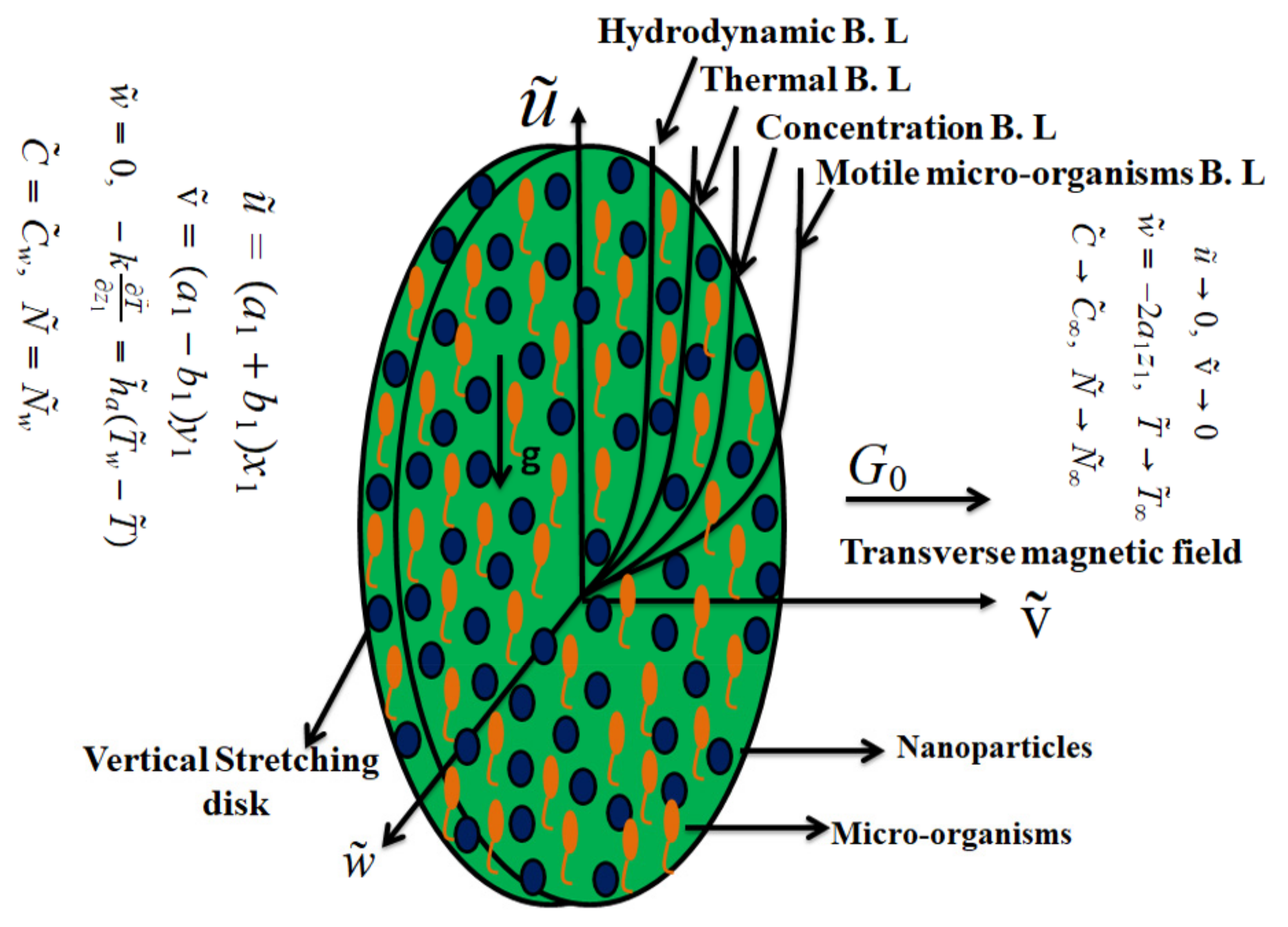
A 3D incompressible MHD bioconvective Walter’s B fluid flow is considered with gyrotactic motile microorganisms and nanoparticles. The heat and mass transport process depends on both thermal radiation and thermal conductivity. The flow of Walter’s B fluid is generated via a cylindrical disk. The flow problem is investigated by applying thermal and solutal convective conditions. The magnetic field is applied normally to the disk. We assume that the surface temperature, microorganism, and concentration are . stand for ambient temperature, concentration, and microorganisms, accordingly. Figure 1 depicts the physical overview of the present analysis. The flow regulating equations for a three-dimensional steady flow of bioconvection Walter’s B nanofluid via cylindrical disk were written with these concerns in mind [19,20].
with:
where are velocity components of , and , respectively; the heat capacity of the nanofluid is ; describes dynamic viscosity; and depict thermal and Brownian diffusion coefficients; indicates the coefficient of viscoelasticity; indicates the strength of the magnetic field; demonstrate nanofluid density, nanoparticle density, and microbe particle density; represents electrical conductivity of nanofluid; is the microorganisms’ diffusivity; depicts the ratio of nanoparticle heat capacity to nanofluid heat capacity; the gravitational force is symbolized by ; indicate concentration and thermal expansion coefficients; shows the motile density of microorganisms; the constant of chemotaxis; is the swimming speed of the strongest cell; is considered to be constant; and indicate the concentrations and temperatures of nearby and faraway fluids; heat capacitance is represented by ; demonstrates thermal conductivity; displays the radiative heat flux. This is a simplified representation of temperature-dependent conductivity , as in [20]
where is thermal conductivity parameter and is ambient thermal conductivity. Transformations to be introduced as follows [20]
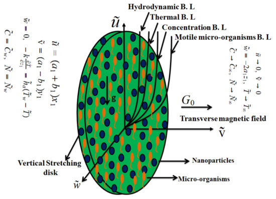
Figure 1.
Analysis of the flow.
After applying the above transformation, we can rewrite the non-dimensional forms of the system as
Here the dimensionless parameters describe
which are the Prandtl number, radiation number, magnetic number, thermophoresis number, Brownian motion number and Schmidt number, stress-to-strain ratio, viscoelastic parameter, mixed convection parameter, buoyancy ratio parameter, bioconvection Rayleigh number, Peclet number, bioconvection Lewis number, and microorganism difference parameter, respectively.
2.1. Physical Quantities of Interest
The heat transfer, motile density, and mass transfer rates are the most essential applications of this topic in industrial and engineering procedures.
Local Nusselt, Motile Density, and Sherwood Numbers
In terms of physical quantities, the local Nusselt number, motile density, and Sherwood number can be expressed as follows
and their dimensionless forms are
3. Structure of the ANN Models
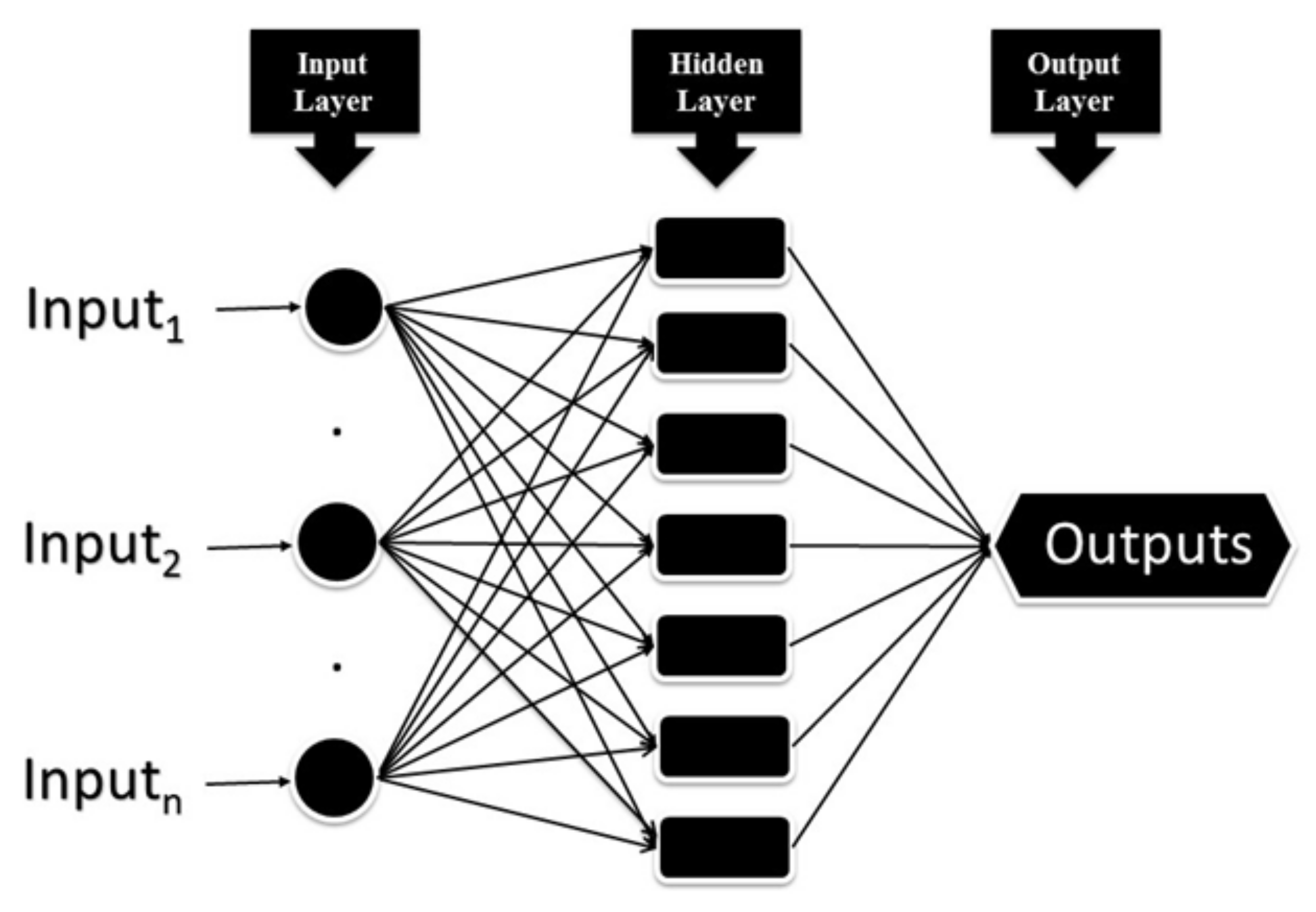
Two different ANN models were developed to model the bioconvective magnetized Walter’s B nanofluid flow flowing towards a cylindrical disk. Since the input variables affecting the LNN, LSHN, and LMDN parameters, which are determined as flow parameters, are different, an ANN model was designed for LNN and LSHN parameters, and a separate ANN model was designed for the development of the LMDN parameter. Input and output parameters of two different ANN models designed are given in Table 1. In both ANN models, the multi-layer perceptron (MLP) network model, which is one of the most preferred ANN models due to its strong structures, is used [21,22,23]. MLP networks consist of layers that are directly connected to each other. The first of the layers is the input layer, which contains the input data. The hidden layer is after the input layer, and every MLP network has at least one hidden layer. The next layer after the hidden layer is the output layer. Figure 2 represents the basic configuration diagram of an MLP network model. Using the Levenberg–Marquardt training algorithm, the MLP network model is trained, which is one of the most preferred algorithms due to its high learning capacity [24,25]. MLP networks employ Tan–Sig and Purelin transfer functions, respectively, on their hidden and output layers. The transfer functions in use are listed below [26,27]:

Table 1.
Input and output parameters for developed ANN models.
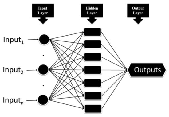
Figure 2.
The basic configuration diagram of an MLP network model.
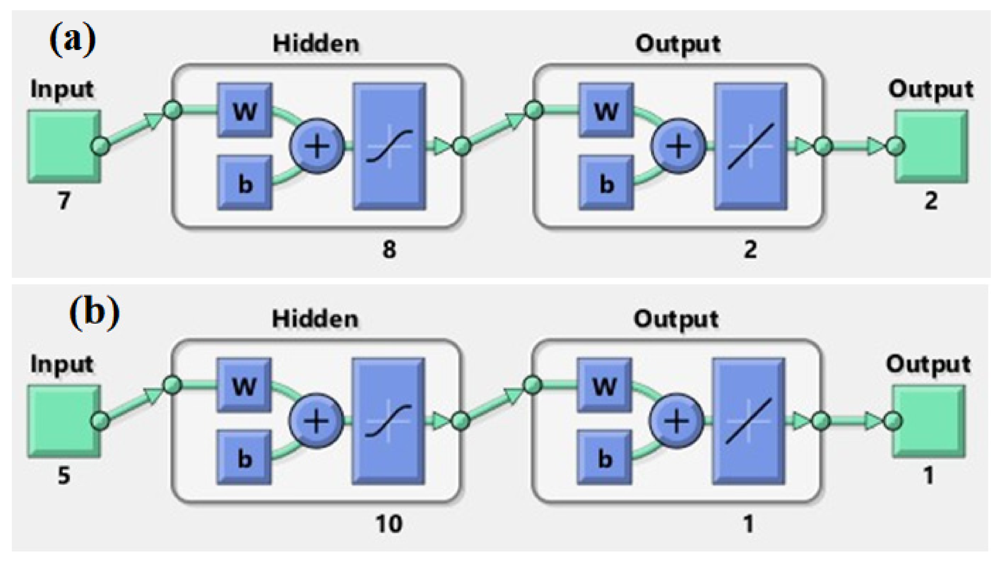
Ideally optimizing and grouping the data to be used in the training of ANN models is one of the parameters that is important for the performance of the models [28]. The model, which is widely used in the literature, was preferred for data optimization and grouping of the developed neural network model [29,30,31]. Of the 36 datasets used for the development of LNN and LSHN parameters, 26 were grouped for training the model, 5 for validation, and 5 for testing. The ANN model developed for estimating the LDMN parameter was trained with a total of 33 data sets, 23 of which were reserved for training, 5 for validation, and 5 for testing. In the hidden layers of MLP neural networks, there is a computational element called a neuron [32]. The lack of a fixed method to determine the number of neurons to be used in the hidden layer is one of the difficulties in the design of MLP networks [33,34]. The performances of MLP networks, which were developed using different numbers of neurons, were examined and the models that gave the most ideal performance were optimized. As a result of the optimization, 8 neurons were used in the hidden layer of the first MLP network model and 10 neurons were used in the hidden layer of the second MLP network. The structural diagrams of the ANN models designed for the development of LNN, LSHN, and LDMN parameters are shown in Figure 3.
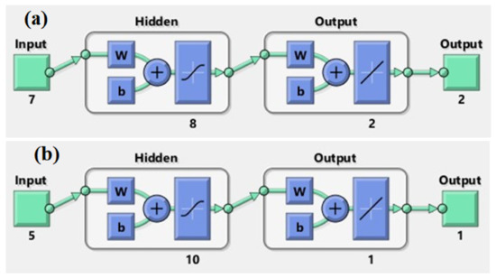
Figure 3.
The structural diagrams of the ANN models designed for the development of LNN, LSHN, and LDMN parameters. (a) 8 neurons were used in the hidden layer; (b) 10 neurons.
In the analysis of training and predictive performance of both ANN models, performance parameters that are commonly used in the literature were preferred [35]. The equations used to calculate the performance parameters mean squared error (MSE) and coefficient of determination (R) are provided below [36]:
The equation used to calculate the margin of deviation (MoD) values between the outputs obtained from the ANN models and the target data is given below [37]:
4. Discussion
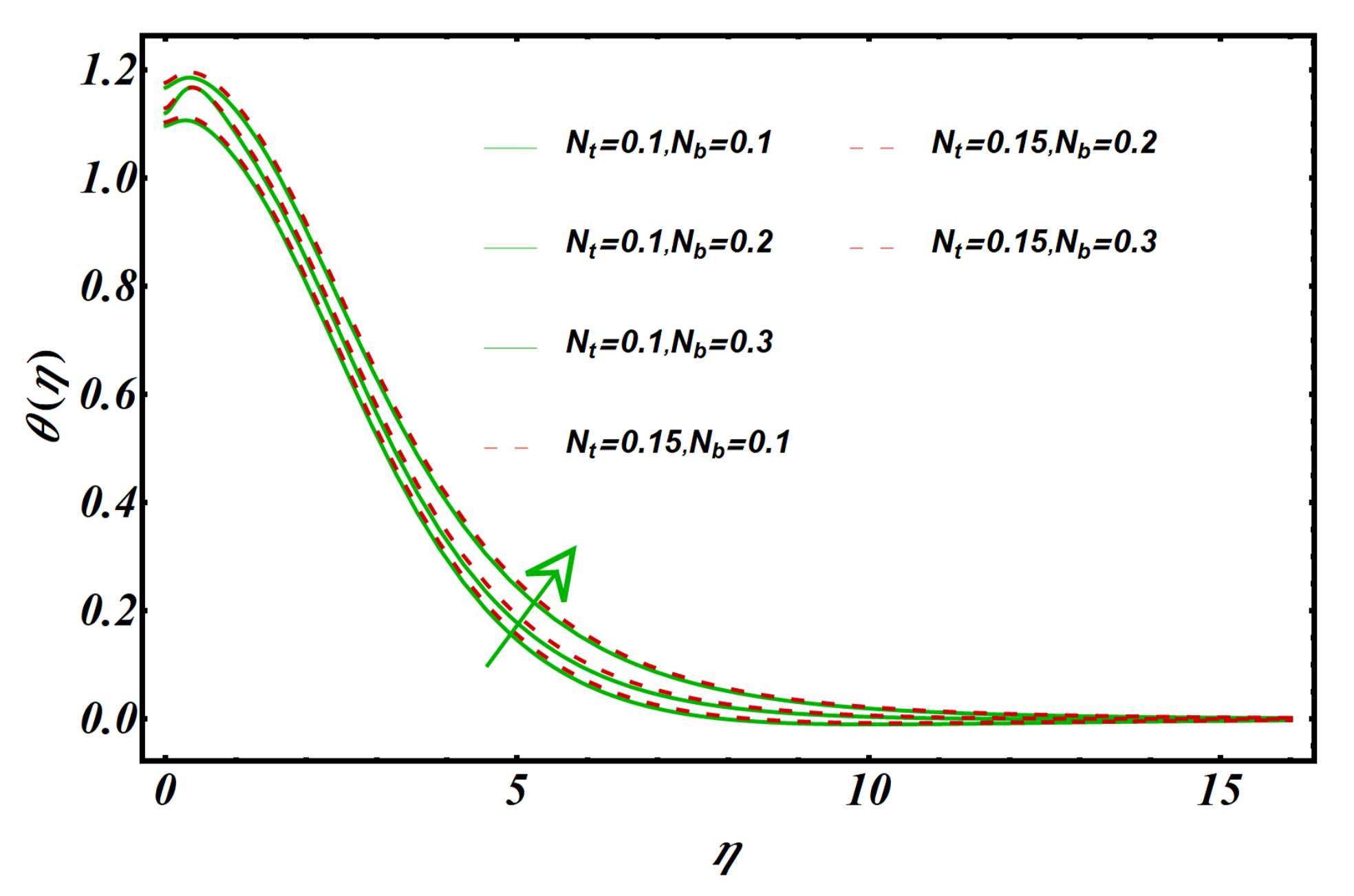
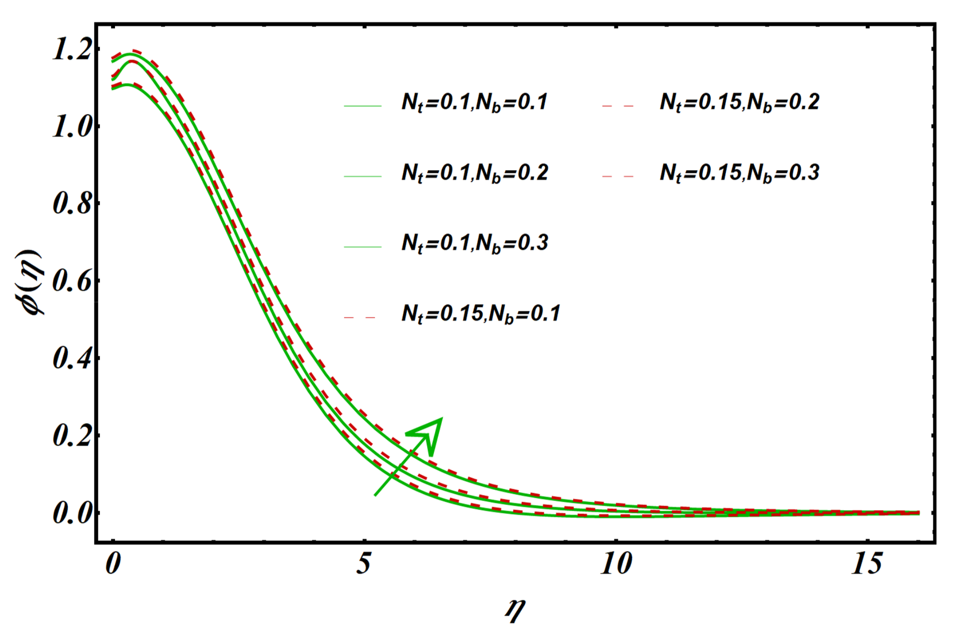
Figure 4 explores the consequences of Brownian motion variable on temperature distribution . A higher Brownian motion variable results in an improved temperature profile . During thermal conduction, nanoparticle motion plays a crucial role. Due to the chaotic movement of the nanoparticles, their kinetic energy rises, increasing the temperature of the nanofluid. It is also notable that Figure 4 depicts the effect of the thermophoresis parameter on the temperature field . It appears in this figure that with an increase in , the temperature field increases. For applications in thermal engineering, this is a significant result. In a physical sense, tends to enhance the thermophoresis force that is responsible for moving nanoparticles from hot to cold areas, which causes a more significant increase in temperature. In Figure 5, the variation in concentration profile is plotted against the thermophoresis parameter . Thermophoresis is known to be induced by large . Due to these forces, the nanoparticles are prone to migrate in the opposite direction of the concentration gradient (that is, from hot to cold) causing a non-uniform nanoparticle distribution. As a result, higher results in an increasing trend in the concentration distribution of nanomaterials. The implications of Brownian motion number on the concentration field are also shown in Figure 5. Larger increases the random motion and collision of the fluid’s macroscopic particles, lowering the fluid concentration.
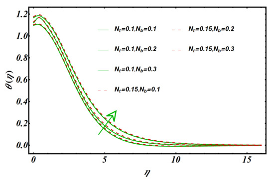
Figure 4.
Impact of and on .
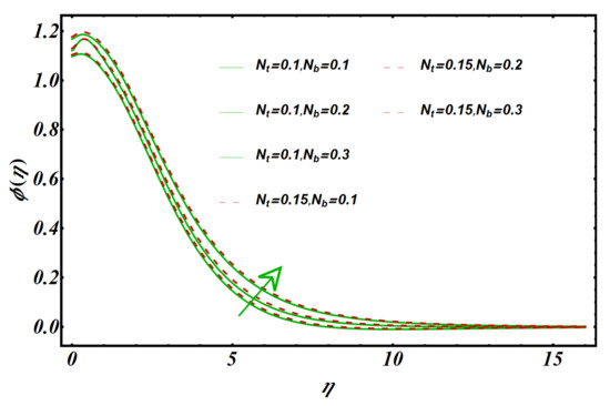
Figure 5.
Impact of and on .
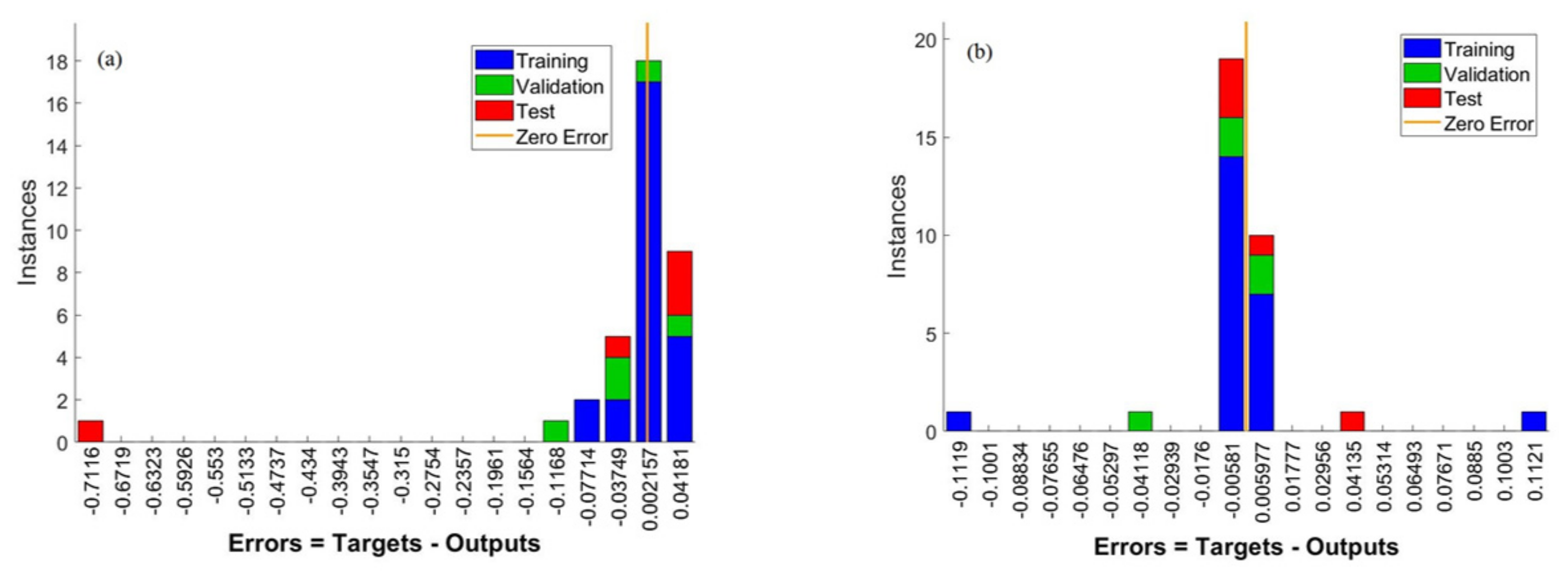
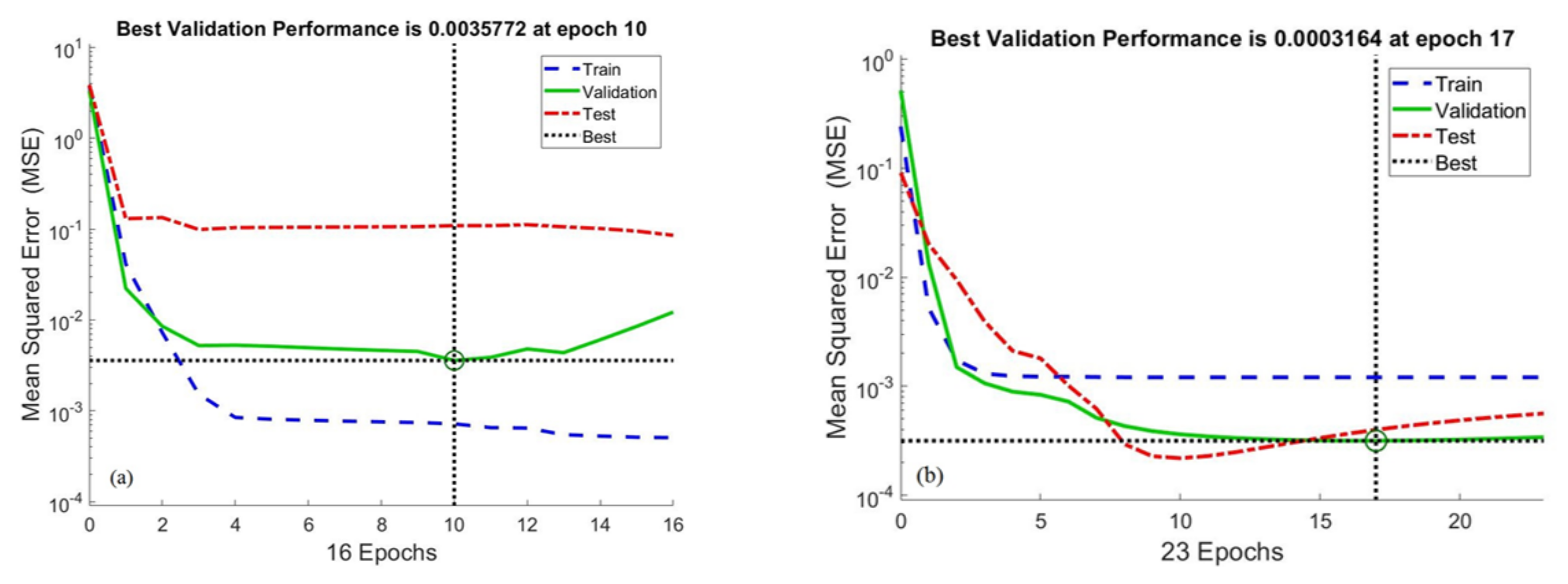
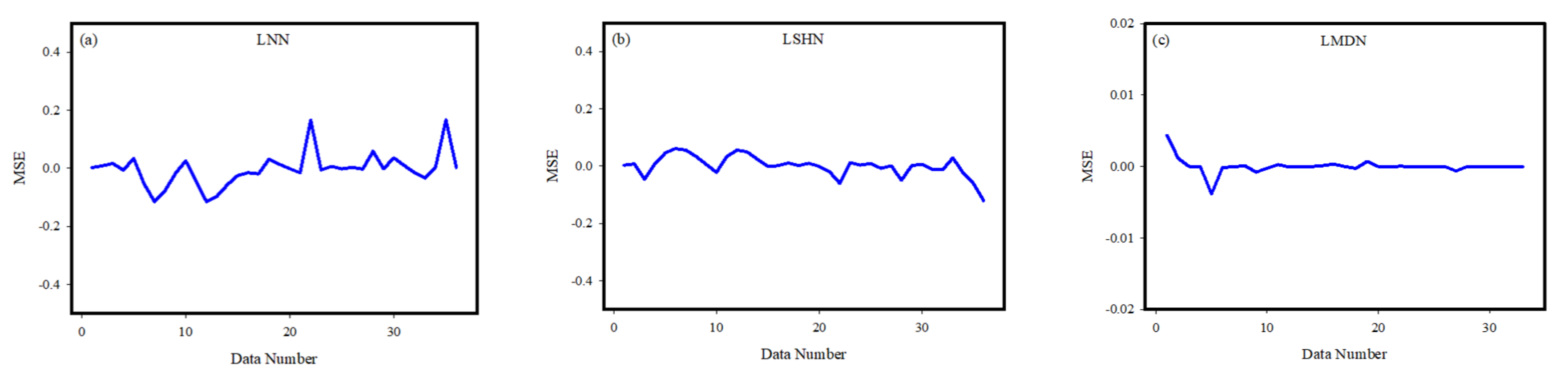
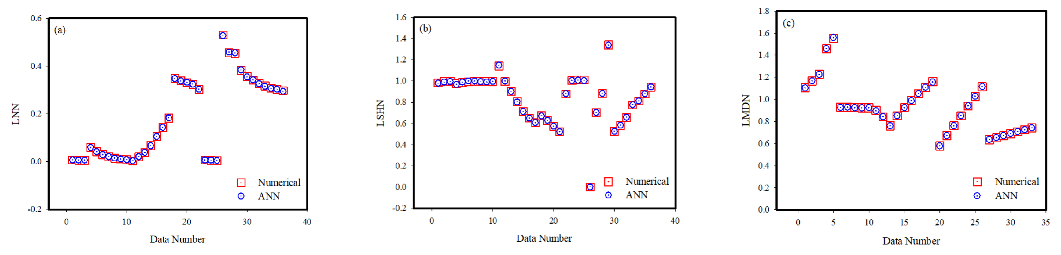
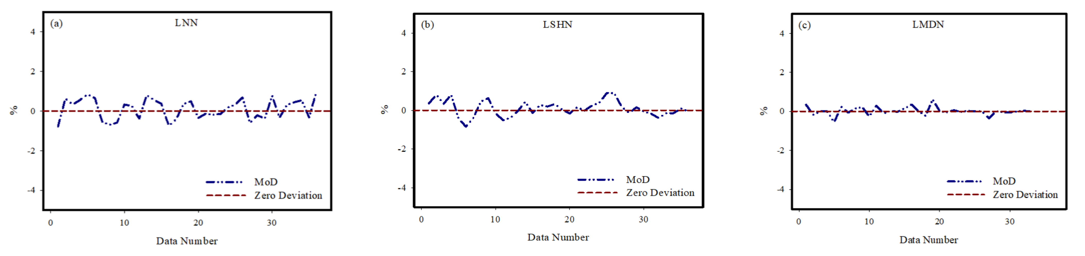
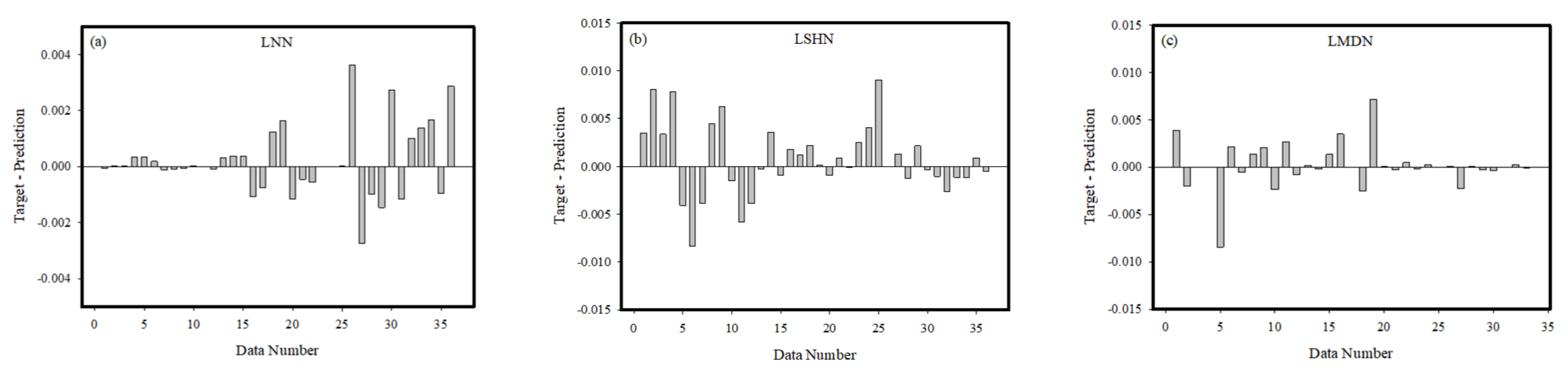
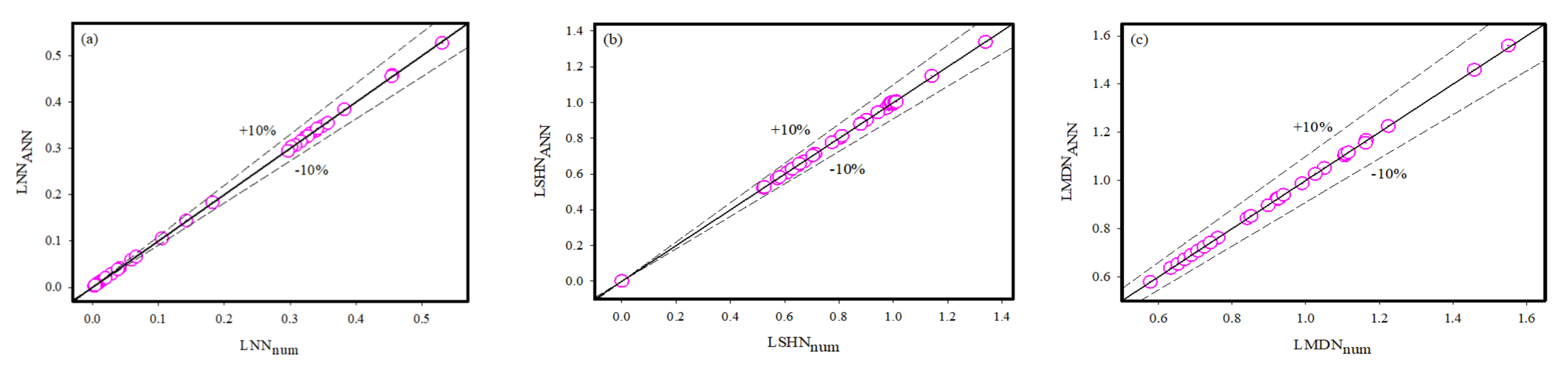
The first step in analyzing the performance of the ANN model is to ensure that the training phase is optimally completed. Figure 6 depicts histograms of the error values attained during the training phase. When the error histogram information is examined, it is discovered that the error values obtained for the three data groups are concentrated around the zero error line. The histograms show that the numerical values of the errors are also very low. The error histogram results show that the errors in the ANN model’s training phase are very low. Figure 7 shows training performance graphs for both MLP neural networks. The graphs show that the MSE values, which are high at the start of the training phase, decrease as the epochs progress. According to the MSE values, which decrease with each epoch and gradually approach zero, the values between the output and target are getting closer to zero. The lowest error value of the MLP networks was achieved with the ideal validation value, and the training stage was completed. Figure 8 shows the calculated MSE values for each data set used for the training phase of the ANN models. The closeness of the MSE values to zero demonstrates the low errors obtained during the model training phase. When the data line showing the calculated MSE values for each output value is examined, it can be seen that they are very close to the zero error values. The MSE values revealed that the training stages of both ANN models were completed optimally. Figure 9 depicts the outputs and target values gained from the ANN models in order to assess estimation accuracy. When the graphs are investigated, it is clear that the points representing the target and output values are perfectly aligned. This agreement between the output values and the target values demonstrates that both ANN models were designed to make accurate predictions. Figure 10 depicts the calculated MoD values for each data point. When the MoD values that demonstrate the proportional deviation among the output values of the ANN models and the target values are inspected, they are found to be very low. The closeness of the curve expressing the MoD values to the zero error line demonstrates that the deviation among the ANN model outputs and the target values is very small. The MoD values show that the developed ANN models can predict with very low deviations. The differences between the target values and the output values were calculated in order to examine the error rates of both ANN models in greater depth. When the difference values given for each data point in Figure 8 are examined, it is seen that the difference values calculated for each data point are very low. The low differences between the target values and the output values show that the developed ANN models can predict with very low errors. While the target values are on the x-axis of Figure 11, the outputs obtained from the ANN model are on the y-axis. When the positions of the data points are analyzed, it is seen that, in general, all data points are located on the zero error line. However, it should be noted that the data points are within the error band. The results obtained from Figure 12 are another proof that both ANN models developed can make predictions with high accuracy. The performance parameters calculated for the developed ANN models are given in Table 2. The fact that the MSE values are quite low, the R value is close to 1, and the MoD values are very low shows that the developed ANN models were developed to predict the LNN, LSHN, and LMDN values with very high accuracy.
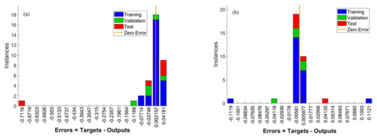
Figure 6.
Error histogram for the ANN models. (a) For LNN and LSHN; (b) For LMDN.
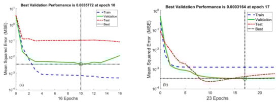
Figure 7.
Training performance graphs of both MLP neural networks. (a) For LNN and LSHN; (b) For LMDN.
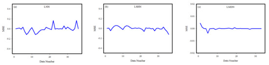
Figure 8.
The calculated MSE values for each data used for the training phase of the ANN models. (a) For LNN; (b) For LSHN. (c) For LMDN.
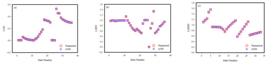
Figure 9.
The target and outputs values obtained from the ANN models. (a) For LNN; (b) For LSHN. (c) For LMDN.
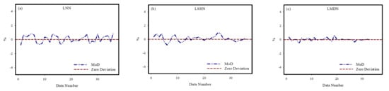
Figure 10.
The MoD values calculated for each data point. (a) For LNN; (b) For LSHN. (c) For LMDN.
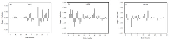
Figure 11.
The differences between the target values and the output values. (a) For LNN; (b) For LSHN. (c) For LMDN.
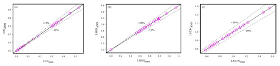
Figure 12.
The numerical values and the ANN outputs. (a) For LNN; (b) For LSHN. (c) For LMDN.
Table 2.
The performance parameters calculated for the developed ANN models.
Table 3 and Table 4 display the LNN, LMDN, and LSHN values for various values of the variables under consideration. It should be observed that LNN improves with an increase in Brownian motion number . Moreover, it has been discovered that LNN reduces as the radiation number , thermal conductivity parameter , thermophoresis parameter , Prandtl numbers , heat generation number , and Lewis number increase. From Table 4 we also note that LSHN reduces as the thermophoresis parameter Brownian motion number and thermal conductivity parameter increase, while it increases when radiation number , Prandtl numbers , heat generation number and Lewis number increase. Table 4 shows that increasing LMDN increases buoyancy ratio parameter , bioconvection Lewis number Peclet number , and microorganisms difference parameter . On the other hand, the opposite behavior is noted for the increment in bioconvection Rayleigh number . The accuracy of the numerical modeling and the ANN model are very close.
Table 3.
The values of LNN and LSHN for various values of physical parameters.
Table 4.
The values of LMDN for various values of physical parameters.
5. Concluding Remarks
The study investigated the bio-convective transport of Walter’s B nanofluid in the presence of thermophoresis and Brownian diffusion through a cylindrical disk using artificial neural networks. Variable thermal conductivity, thermal radiation, and motile microorganisms are also considered. The non-linear simplified equations were numerically calculated using the Runge–Kutta fourth-order shooting procedure. The study’s key findings include the following:
- In thermal engineering applications, thermophoresis and Brownian motion play significant roles.
- Thermophoresis number tends to enhance the thermophoresis force that is responsible for moving nanoparticles from hot to cold areas, which causes a more significant increase in temperature.
- As indicated by the MoD value, the developed ANN models are capable of making very accurate predictions.
- According to the error histograms, there is very little error in the training phase of the ANN model.
- MSE values calculated for LNN, LSHN, and LMDN parameters were obtained as , , and , respectively.
- The R value for the ANN model developed for estimating LNN and LSHN values is 0.98537.
- The R value calculated for the ANN model developed to estimate the LMDN value is 0.99269.
- The average MoD value for LNN and LSHN values was calculated as 0.1% and the average MoD value for LMDN value was calculated as 0.02%.
- The findings obtained as a result of the calculation and analysis of the performance parameters clearly showed that both ANN models can make predictions with high accuracy.
Author Contributions
A.S.: Conceptualization, Writing—review and editing, Data curation, Formal analysis, Methodology, Validation. A.B.Ç.: Software, Methodology, Writing—review and editing, Data curation, Formal analysis, Methodology. T.N.S.: Data curation, Formal analysis, Validation, Conceptualization, Methodology, Writing—original draft. All authors have read and agreed to the published version of the manuscript.
Funding
This research work has no funding.
Institutional Review Board Statement
Not applicable.
Informed Consent Statement
Not applicable.
Data Availability Statement
Data are contained within the article.
Conflicts of Interest
The author(s) declared no potential conflicts of interest with respect to the research, authorship and/or publication of this article.
Nomenclature
| dimensionless temperature | |
| surface temperature | |
| dimensionless velocity | |
| gravitational force | |
| dimensionless concentration | |
| density of nanofluid | |
| dimensionless motile density | |
| magnetic field | |
| coefficients of concentration and thermal | |
| stretching velocity | |
| specific heat | |
| ambient microorganisms concentration | |
| density of nanomaterials | |
| heat capacity of nanofluid | |
| microbe particle density | |
| thermal diffusion coefficient | |
| Brownian motion coefficient | |
| Stefan–Boltzmann constant | |
| microorganism diffusivity | |
| temperature dependent conductivity | |
| viscosity of nanofluid | |
| maximum speed of swimming cell | |
| constant | |
| motile density of microorganisms | |
| radiative heat flux | |
| velocity components in directions, respectively | |
| heat transfer coefficient | |
| viscoelastic parameter | |
| stress-to-strain ratio | |
| ambient temperature | |
| chemotaxis constant | |
| concentration of nanoparticles | |
| coefficient of viscoelasticity | |
| nanoliquid’s electrical conductivity | |
| ratio of heat capacity of nanoparticles by the heat capacity of nanofluid | |
| ambient nanoparticles concentration | |
| Brownian motion number | |
| Prandtl number | |
| bioconvection Pecelt number | |
| Lewis parameter | |
| radiation number | |
| M | magnetic number |
| bioconvection Lewis number | |
| stress-to-strain ratio | |
| thermophoresis number | |
| viscoelastic parameter | |
| bioconvection Rayleigh number | |
| mixed convection number | |
| microorganisms difference parameter | |
| buoyancy ratio parameter |
References
- Shafiq, A.; Çolak, A.B.; Sindhu, T.N.; Al-Mdallal, Q.M.; Abdeljawad, T. Estimation of unsteady hydromagnetic Williamson fuid fow in a radiative surface through numerical and artificial neural network modeling. Sci. Rep. 2021, 11, 14509. [Google Scholar] [CrossRef] [PubMed]
- Miandoab, A.R.; Bagherzadeh, S.A.; Isfahani, A.H.M. Numerical study of the effects of twisted-tape inserts on heat transfer parameters and pressure drop across a tube carrying Graphene Oxide nanofluid: An optimization by implementation of Artificial Neural Network and Genetic Algorithm. Eng. Anal. Bound. Elem. 2022, 140, 1–11. [Google Scholar] [CrossRef]
- Shafiq, A.; Çolak, A.B.; Sindhu, T.N.; Muhammad, T. Optimization of Darcy-Forchheimer squeezing flow in nonlinear stratified fluid under convective conditions with artificial neural network. HeatTransfer Res. 2022, 3, 53. [Google Scholar] [CrossRef]
- Alzahrani, F.; Khan, M.I. Entropy generation and Joule heating applications for Darcy Forchheimer flow of Ree-Eyring nanofluid due to double rotating disks with artificial neural network. Alex. Eng. 2022, 61, 3679–3689. [Google Scholar] [CrossRef]
- Shafiq, A.; Çolak, A.B.; Sindhu, T.N. Designing artificial neural network of nanoparticle diameter and solid–fluid interfacial layer on single-walled carbon nanotubes/ethylene glycol nanofluid flow on thin slendering needles. Int. J. Numer. Methods Fluids 2021, 93, 3384–3404. [Google Scholar] [CrossRef]
- Choi, S.U.S. Enhancing thermal conductivity of fluids with nanoparticles. ASME 1995, 66, 99–105. [Google Scholar]
- Buongiorno, J. Convective transport in nanofluids. J. Heat Tran. 2006, 128, 240–250. [Google Scholar] [CrossRef]
- Radwan, M.S.; Saleh, H.E.; Attai, Y.A.; Elsherbiny, M.S. On heat transfer enhancement in diesel engine cylinder head using γ-Al2O3/water nanofluid with different nanoparticle sizes. Adv. Mech.Eng. 2020, 12, 1687814019897507. [Google Scholar] [CrossRef]
- Pantokratoras, A. Discussion:“Computational analysis for mixed convective flows of viscous fluids with nanoparticles”. J. Therm. Sci. Eng. Appl. 2019, 11, 5. [Google Scholar]
- Tayebi, T.; Chamkha, A.J. Magnetohydrodynamic natural convection heat transfer of hybrid nanofluid in a square enclosure in the presence of a wavy circular conductive cylinder. J. Therm. Sci. Eng. Appl. 2020, 12, 3. [Google Scholar] [CrossRef]
- Dutta, J.; Kundu, B. Finite integral transform based solution of second grade fluid flow between two parallel plates. J. Appl. Comput. Mech. 2019, 5, 989–997. [Google Scholar]
- Rana, M.A.; Latif, A. Three-dimensional free convective flow of a second-grade fluid through a porous medium with periodic permeability and heat transfer. Bound. Value Probl. 2019, 2019, 44. [Google Scholar] [CrossRef]
- Rasool, G.; Zhang, T.; Shafiq, A. Marangoni effect in second grade forced convective flow of water based nanofluid. J. Adv. Nanotechnol. 2019, 1, 50. [Google Scholar] [CrossRef] [Green Version]
- Shafiq, A.; Sindhu, T.N.; Al-Mdallal, Q.M. A sensitivity study on carbon nanotubes significance in Darcy–Forchheimer flow towards a rotating disk by response surface methodology. Sci. Rep. 2021, 11, 1–26. [Google Scholar]
- Chu, Y.-M.; Khan, U.; Shafiq, A.; Zaib, A. Numerical simulations of time-dependent micro-rotation blood flow induced by a curved moving surface through conduction of gold particles with non-uniform heat sink/source. Arab. J. Sci. Eng. 2021, 46, 2413–2427. [Google Scholar] [CrossRef]
- Shafiq, A.; Mebarek-Oudina, F.; Sindhu, T.N.; Abidi, A. A study of dual stratification on stagnation point Walters’ B nanofluid flow via radiative Riga plate: A statistical approach. Eur. Phys. J. Plus 2021, 136, 1–24. [Google Scholar] [CrossRef]
- Okokpujie, I.P.; Tartibu, L.K.; Sinebe, J.E.; Adeoye, A.O.M.; Akinlabi, E.T. Comparative Study of Rheological Effects of Vegetable Oil-Lubricant, TiO2, MWCNTs Nano-Lubricants, and Machining Parameters’ Influence on Cutting Force for Sustainable Metal Cutting Process. Lubricants 2022, 10, 54. [Google Scholar] [CrossRef]
- Khan, U.; Zaib, A.; Ishak, A.; Waini, I.; Sherif, M.E.S.; Boonsatit, N.; Pop, I.; Jirawattanapanit, A. Ramification of Hall and Mixed Convective Radiative Flow towards a Stagnation Point into the Motion of Water Conveying Alumina Nanoparticles Past a Flat Vertical Plate with a Convective Boundary Condition: The Case of Non-Newtonian Williamson Fluid. Lubricants 2022, 10, 192. [Google Scholar] [CrossRef]
- Abbasi, A.; Mabood, F.; Farooq, W.; Batool, M. Bioconvective flow of viscoelastic nanofluid over a convective rotating stretching disk. Int. Commun. Heat Mass Tran. 2020, 119, 104921. [Google Scholar] [CrossRef]
- Hassan, W.; Metib, A.; Taseer, M.; Khan, M.A. Bioconvection transport of magnetized Walter’s B nanofluid across a cylindrical disk with nonlinear radiative heat transfer. Case Stud. Therm. Eng. 2021, 26, 101097. [Google Scholar]
- Vaferi, B.; Samimi, F.; Pakgohar, E.; Mowla, D. Artificial neural network approach for prediction of thermal behavior of nanofluids flowing through circular tubes. Powder Technol. 2014, 267, 1–10. [Google Scholar] [CrossRef]
- Canakci, A.; Ozsahin, S.; Varol, T. Modeling the influence of a process control agent on the properties of metal matrix composite powders using artificial neural networks. Powder Technol. 2012, 228, 26–35. [Google Scholar] [CrossRef]
- Güzel, T.; Çolak, A.B. An experimental study on artificial intelligence-based prediction of capacitance-voltage parameters of polymer-interface 6H-SiC/MEH-PPV/Al Schottky diodes. Phys. Status Solidi A Appl. Mater. Sci. 2022, 219, 2100821. [Google Scholar] [CrossRef]
- Ali, A.; Abdulrahman, A.; Garg, S.; Maqsood, K.; Murshid, G. Application of artificial neural networks (ANN) for vapor-liquid-solid equilibrium prediction for CH4-CO2 binary mixture. Greenh. Gases 2019, 9, 67–78. [Google Scholar] [CrossRef]
- Kareem, F.A.A.; Shariff, A.M.; Ullah, S.; Garg, S.; Dreisbach, F.; Keong, L.K.; Mellon, N. Experimental and neural network modeling of partial uptake for a carbon dioxide/methane/water ternary mixture on 13X zeolite. Energy Technol. 2017, 5, 1373–1391. [Google Scholar] [CrossRef]
- Vafaei, M.; Afrand, M.; Sina, N.; Kalbasi, R.; Sourani, F.; Teimouri, H. Evaluation of thermal conductivity of MgO-MWCNTs/EG hybrid nanofluids based on experimental data by selecting optimal artificial neural networks. Phys. E 2017, 85, 90–96. [Google Scholar] [CrossRef]
- Akhgar, A.; Toghraie, D.; Sina, N.; Afrand, M. Developing dissimilar artificial neural networks (ANNs) to prediction the thermal conductivity of MWCNT-TiO2/Water-ethylene glycol hybrid nanofluid. Powder Technol. 2019, 355, 602–610. [Google Scholar] [CrossRef]
- Çolak, A.B. An experimental study on the comparative analysis of the effect of the number of data on the error rates of artificial neural networks. Int. J. Energy Res. 2021, 45, 478–500. [Google Scholar] [CrossRef]
- Esmaeilzadeh, F.; Teja, A.S.; Bakhtyari, A. The thermal conductivity, viscosity, and cloud points of bentonite nanofluids with n-pentadecane as the base fluid. J. Mol. Liq. 2020, 300, 112307. [Google Scholar] [CrossRef]
- Barati-Harooni, A.; Najafi-Marghmaleki, A. An accurate RBF-NN model for estimation of Viscosity of nanofluids. J. Mol. Liq. 2016, 224, 580–588. [Google Scholar] [CrossRef]
- Rostamian, S.H.; Biglari, M.; Saedodin, S.; Esfe, M.H. An inspection of thermal conductivity of CuO-SWCNTs hybrid nanofluid versus temperature and concentration using experimental data, ANN modeling and new correlation. J. Mol. Liq. 2017, 231, 364–369. [Google Scholar] [CrossRef]
- Ahmadloo, E.; Azizi, S. Prediction of thermal conductivity of various nanofluids using artificial neural network. Int. Heat Mass Transf. 2016, 74, 69–75. [Google Scholar] [CrossRef]
- Bonakdari, H.; Zaji, A.H. Open channel junction velocity prediction by using a hybrid self-neuron adjustable artificial neural network. Flow Meas. Instrum. 2016, 49, 46–51. [Google Scholar] [CrossRef]
- Çolak, A.B.; Güzel, T.; Yıldız, O.; Özer, M. An experimental study on determination of the shottky diode current-voltage characteristic depending on temperature with artificial neural network. Phys. B 2021, 608, 412852. [Google Scholar] [CrossRef]
- Çolak, A.B.; Yıldız, O.; Bayrak, M.; Tezekici, B.S. Experimental study for predicting the specific heat of water based Cu-Al2O3 hybrid nanofluid using artificial neural network and proposing new correlation. Int. J. Energy Res. 2020, 44, 7198–7215. [Google Scholar] [CrossRef]
- Öcal, S.; Gökçek, M.; Çolak, A.B.; Korkanxcx, M. A comprehensive and comparative experimental analysis on thermal conductivity of TiO2-CaCO3/Water hybrid nanofluid: Proposing new correlation and artificial neural network optimization. Heat Transf. Res. 2021, 52, 55–79. [Google Scholar] [CrossRef]
- Çolak, A.B.; Karakoyun, Y.; Acikgoz, O.; Yumurtacı, Z.; Dalkılıç, A.S. A Numerical Study Aimed at Finding Optimal Artificial Neural Network Model Covering Experimentally Obtained Heat Transfer Characteristics of Hydronic Underfloor Radiant Heating Systems Running Various Nanofluids. Heat Transf. Res. 2022, 53, 51–71. [Google Scholar] [CrossRef]
Publisher’s Note: MDPI stays neutral with regard to jurisdictional claims in published maps and institutional affiliations. |
© 2022 by the authors. Licensee MDPI, Basel, Switzerland. This article is an open access article distributed under the terms and conditions of the Creative Commons Attribution (CC BY) license (https://creativecommons.org/licenses/by/4.0/).