Analysis of Wind Data for Sports Performance Design: A Case Study for Sailing Sports

Abstract

Environmental conditions affect outdoor sports performance. This is particularly true in some sports, especially in the sport of sailing, where environmental parameters are extremely influential as they interact directly with strategic analysis of the race area and then with strategic analysis of the performance itself. For these reasons, this research presents an innovative methodology for the strategic analysis of the race course that is based on the integrated assessment of meteorological data measured on the ground, meteorological data measured at sea during the training activities and the results of the CALMET model in hindcasting over a limited scale. The results obtained by the above analysis are then integrated into a graphical representation that provides to coaches and athletes the main strategic directions of the race course in a simple and easy-to-use way. The authors believe that the innovative methodology that has been adopted in the present research may represent a new approach to the integrated analysis of meteorological data on coastal environments. On the other hand, the results of this analysis, if presented with an appropriate technique of meta‑communication adapted to the sport sectors, can be used effectively for the improvement of athletes’ performances.

1. Introduction

The effect of weather and environmental conditions on sports has been extensively studied over the years [1,2,3,4]. Based upon the studies of Lobozewicz [5] and of Kay and Vamplew [6], Pezzoli and Cristofori [7] have studied the impact of some specific environmental parameters on different sports using a particular impact index divided into five classes. This analysis clearly shows that most of the outdoor sport activities, and in particular endurance sports, are strongly influenced by the variation of meteorological parameters.

Actually the evaluation of bio-climatological conditions and of thermal comfort in endurance sports, particularly in road cycling, is of fundamental importance not only for a proper planning of the training program and the nutritional plan, but also for a better evaluation of the race strategy [8,9].

Despite these observations, the influence of meteorological and environmental conditions is often disregarded in outdoor sport performance assessments [10,11].

Some new researches about team sports [12,13,14], cycling [15], marathons [16,17], water sports [10], effect of materials and apparels on the sport performance [18,19,20] as well as the recent results obtained by Pezzoli et al. [11], show that in sports performance analysis it is necessary to work, not only in the well-known areas of “Performance Analysis” (“Motion Analysis”, “Match Analysis” and “Notational Analysis”), but also in the area of “Environmental Analysis”.

Different authors studied the effect of the environment and of the weather on the sailing sports and concluded that a meteorological division (or, at least, a “Weather Coach”) should be present in the team because meteorological conditions can influence the “performance” of the athletes [21,22,23,24].

Moreover, Bethwaite [25] shows how in sailing it is possible to subdivide the performance in strategy, tactic and technique, where the strategy is the analysis of the relationship between the boat and the environment, while tactic is the analysis of the relationship between the boat and the other boats. The analysis conducted by Pezzoli et al. [11] demonstrates that the athletes and the coaches in sailing need to have reliable information about the weather and the atmospheric conditions of the race area with a different time scaling.

Gaining knowledge on the wind patterns in the racing area is very important for the sailors, which, before the race as well as during the race, must elaborate strategic and tactical decisions in very short times.

The aim of this work is to develop a general methodology that can be used to help sailors to get reliable information about the race area by means of a careful analysis of the meteorological observations which is also supported by the use of a simulation tool. The final product is the “Call Book”, which is a handy guide made available to athletes and coaches where the meteorological conditions and the strategic analysis are described in detail.

The data measured by meteorological stations have been used to determine the recurrent “Weather Patterns” (WP hereafter). The method of analysis of the climatologic and meteorological conditions through the use of WPs has been widely used to forecast intense rain events [26,27] and for climatologic forecasting of the general atmospheric circulation and its downscaling at a regional scale [28].

This research presents an innovative methodology that, by means of a multidimensional statistical analysis, allows to individuate recurrent WPs at local scale and to recognize the main meteorological features at synoptic scale associated to each WP.

In the same time, using a limited area model in hindcasting (CALMET), the wind roses have been built in the center of each race area by means of an off-shore data base. The analysis of the resulting wind roses allows defining the strategic types of the regatta field as those where:

(1)

wind varies in the different zones both in direction and speed;

(2)

wind varies in the different zones for direction and not for intensity (these regatta fields are extremely rare);

(3)

wind intensity varies and wind direction remains almost constant (or also there is a variation of the “wind pressure”).

The determination of the regatta field type is essential to set up a correct strategy. It is therefore evident that the methodology proposed in this research can actually be useful for both coaches and athletes.

2. Material and Methods

2.1. Research Design

This work presents the results of the analysis of the wind patterns in the bay of Santander (Spain) where the ISAF (International Sailing Federation) Sailing World Championships was held in September 2014 (Santander 2014 hereafter). Santander 2014 was a very important sport event, both for the high level of the participating teams, and because it was the qualifier for the Olympic games of Rio 2016. Additional information about the event is available at http://www.santander2014.com/.

The analysis and reconstruction of the meteorological field has been conducted with an innovative methodology by means of the CALMET diagnostic meteorological model [29] with a high spatial resolution. The CALMET results have been compared against the observations of the “El Sardinero” meteorological station, which is located close to the shore line. Additional observations have been collected during the Santander test event of September 2013. The comparison between predicted and observed variables has been carried out both qualitatively by judging the time trends, and quantitatively by means of some statistical parameters.

2.2. Material

2.2.1. The CALMET Meteorological Model

The CALMET meteorological model [29] has been used to create the virtual meteorological database for the period September 8–21, 2013. CALMET is the meteorological preprocessor of the CALPUFF dispersion model [30], which belongs to the list of preferred/suggested models of the US-EPA (United States Environmental Protection Agency).

CALMET is a diagnostic meteorological model which reconstructs the 3D wind and temperature fields starting from meteorological measurements, orography and land use data. Besides the wind and temperature fields, CALMET determines the 2D fields of micro meteorological variables needed to describe the atmospheric turbulence and to carry out dispersion simulations (mixing height, Monin Obukhov length, friction velocity, convective velocity and others).

The diagnostic wind field module of CALMET uses a two‑step approach for the computation of the wind field. In the first step (S1), an initial guess wind field is adjusted for kinematic effects of terrain, slope flows, and terrain blocking effects to produce a S1 wind field. The second step (S2) consists of an objective analysis procedure to introduce observational data into the S1 wind field to produce a final wind field. CALMET can optionally use the output of some prognostic meteorological models in three different ways: as a replacement for the initial guess field, as a replacement for the S1 field, as pseudo observations in the objective analysis procedure.

2.2.2. Geophysical Data

CALMET has been applied over a domain of 17 × 13 km², with a grid amplitude of 500 m. The lower left corner of the domain has the following UTM coordinates within zone 30T: Easting 427500, Northing 4807500.

One of the input files of CALMET includes the geophysical data required by the model: land use type, terrain elevation, surface parameters (surface roughness length, albedo, Bowen ratio, soil heat flux parameter, and vegetation leaf area index) and anthropogenic heat flux. The land use and elevation data are entered as gridded fields, whereas the surface parameters and anthropogenic heat flux can be entered either as gridded fields or computed from the land use data at each grid point.

Terrain and land use have been averaged within each 500 m grid cell of the CALMET domain starting from the original data, which derive respectively from the Shuttle Radar Topography Mission (SRTM) database and the CORINE Land Cover database. The resulting averaged terrain elevation and land cover are shown in Figure 1. The grid averaged terrain elevation is measured from 0 m of the sea, in the northern part of the domain, to a bit more than 100 m at the south eastern part of the domain. The percentage distribution of land use over the grids of the simulation domain indicates that more than 58% of the domain is covered by water, and another great part (19%) is covered by complex cultivation patterns. The built-in area covers more than 10% of the domain. Surface parameters and anthropogenic heat flux were not available as gridded fields, therefore the model default values were used.

2.2.3. Input Meteorological Data

CALMET needs meteorological observations with surface and upper air data. At surface, the following variables are needed with hourly resolution: wind speed, wind direction, temperature, cloud cover, ceiling height, surface pressure, relative humidity and precipitation rate. The upper air data, needed at least twice daily, must include for each vertical level: wind speed, wind direction, temperature, pressure and height.

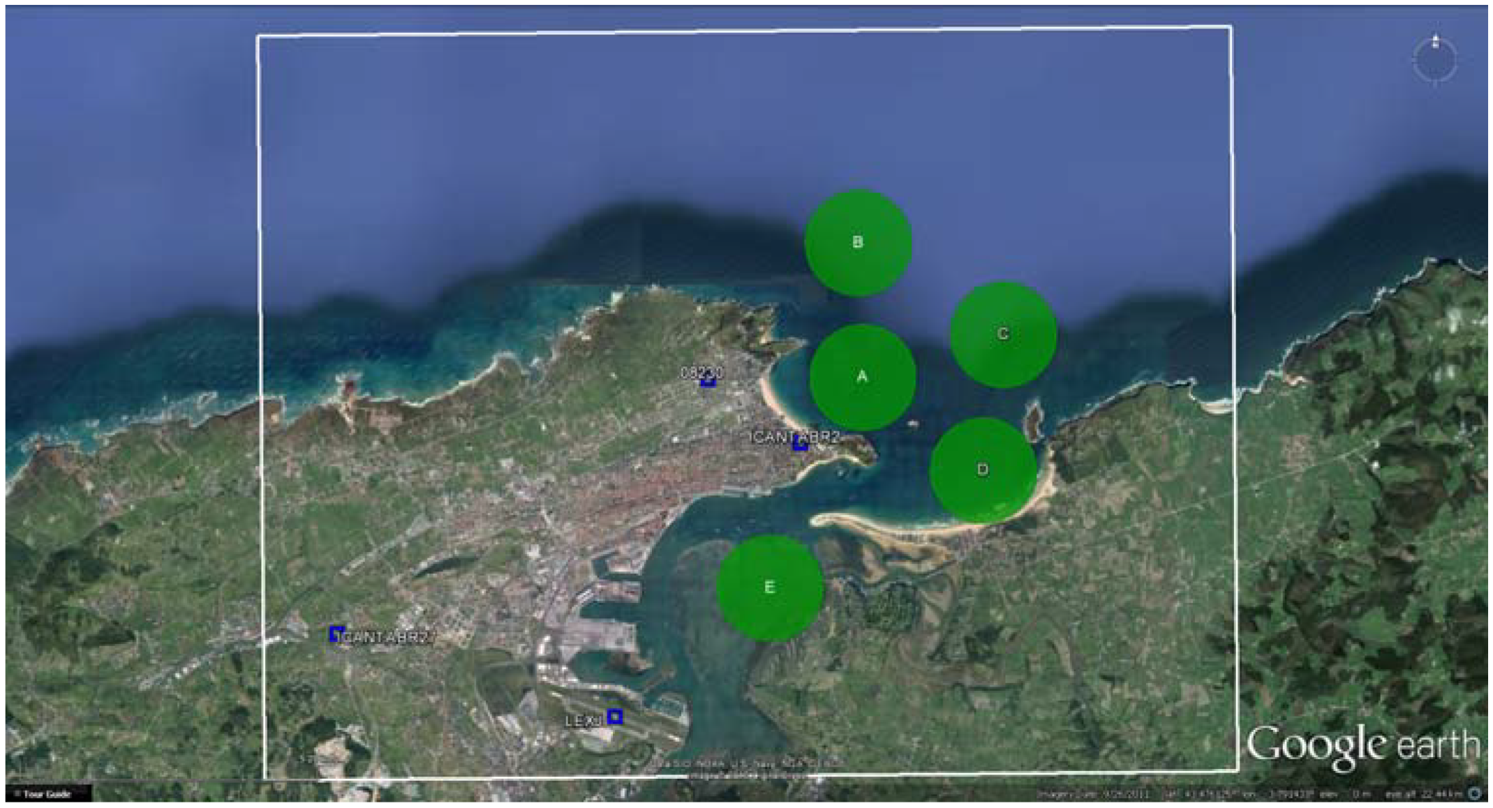
The surface observations have been taken from the ICANTABR27 weather station, located in the south western part of the domain, and from the METAR data of the Santander airport (ICAO code LEXJ), located in the southern part of the domain. The upper air data have been taken from the WMO station 08023, located in the central part of the domain close to the shore line. The positions of the meteorological stations are shown in Figure 2 with blue squares.

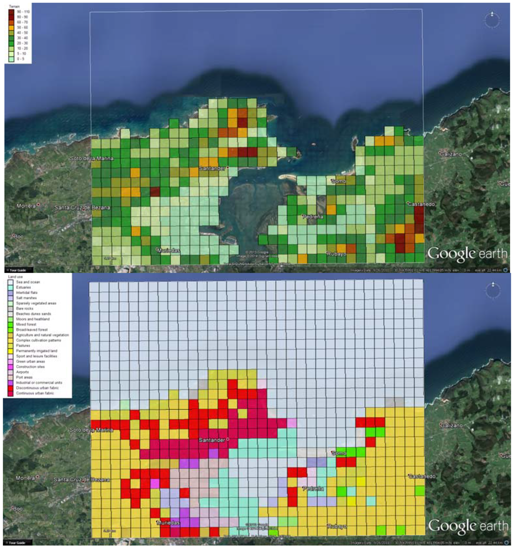
Figure 1. Reconstruction of terrain elevation (above) and land cover (below) over the 500 × 500 m² cells of the simulation domain.

Figure 1. Reconstruction of terrain elevation (above) and land cover (below) over the 500 × 500 m² cells of the simulation domain.

Figure 2. Simulation domain (white rectangle), meteorological monitoring stations (blue squares) and regatta areas (green circles).

Figure 2. Simulation domain (white rectangle), meteorological monitoring stations (blue squares) and regatta areas (green circles).

The ICANTABR27 observations are available with a time resolution of 5 min, and they have been averaged over each hour in order to prepare the data as needed by CALMET. The upper air meteorological observations of the WMO station 08023 are available every 12 h, and they have only been formatted as needed by CALMET, without any averaging.

The METAR observations are available each day with half‑hour time resolution only for the time period 05:30–23:00 LT. The fact that the METAR data do not cover the whole day is not a problem because, for the current application, the CALMET output are needed for the period 09:00–18:00, therefore bogus data can be used for the missing hours, since CALMET is a diagnostic model. Moreover, a preliminary analysis of the input data has shown that the METAR observations are often characterized by variable winds during the morning, therefore it was not possible to assign a precise direction to the wind, for this reason all the METAR data during the morning have been invalidated.

At the same time, the data measured by the ICANTABR27 station averaged over each hour have been used to determine the recurrent “Weather Patterns” (WP hereafter) over the race course by means of specialized software.

2.2.4. The WindRose PRO3 Software

A wind rose is a chart which gives a view of how wind speed and wind direction are distributed at a particular location over a specific period of time. A ternary plot (or three variables plot) is a polar coordinate chart where the distance of each point from the center (pole) is determined by the wind speed, the angle from north in clockwise direction is determined by the wind direction, and the color and/or size of each point depends on the value of a third variable (e.g., atmospheric temperature, pressure, concentration of a specific pollutant, etc.). Both these representations allow summarizing in a single plot a large quantity of data; therefore they are very useful representations.

The wind roses and the ternary plots presented in this work have been produced with the WindRose PRO3 software [31].

A time filter option allows analyzing the wind data and produce wind roses only for particular years, months, days of the week or hours of the day. It is also possible to produce wind roses only for day or night hours, which are determined by the software itself starting from the geographical position and the time zone of the meteorological station.

The WindRose PRO3 software has been used in many sectors: meteorology, architecture, air quality, oceanography, veterinary medicine, veterinary epidemiology, wind energy, climate, aquatic botany and agriculture. It has also been used for the analysis of sport performances [10].

2.2.5. Off Shore Weather Observations

An off shore measuring campaign has been carried out in the period September 8–15, 2013 during a training camp of the Swedish Olympic Sailing Team. Many meteorological variables (wind direction and speed, temperature, humidity and atmospheric pressure) have been repeatedly measured during this campaign over the regatta fields, with particular attention to fields A, B and C (Figure 2).

The measurements were performed by means of a rubber dinghy at different points of the regatta fields, with a sampling time of 10″ and a total measuring time of 1′–2′ at each point. During the measurements the rubber dinghy was arrested to avoid its rolling and pitching influencing the measurements. A high‑precision handle anemometer (JDC—SKYWATCH Geos 11) [32] was used; this tool has already proved to be extremely performing in the application of meteorology to sport [15].

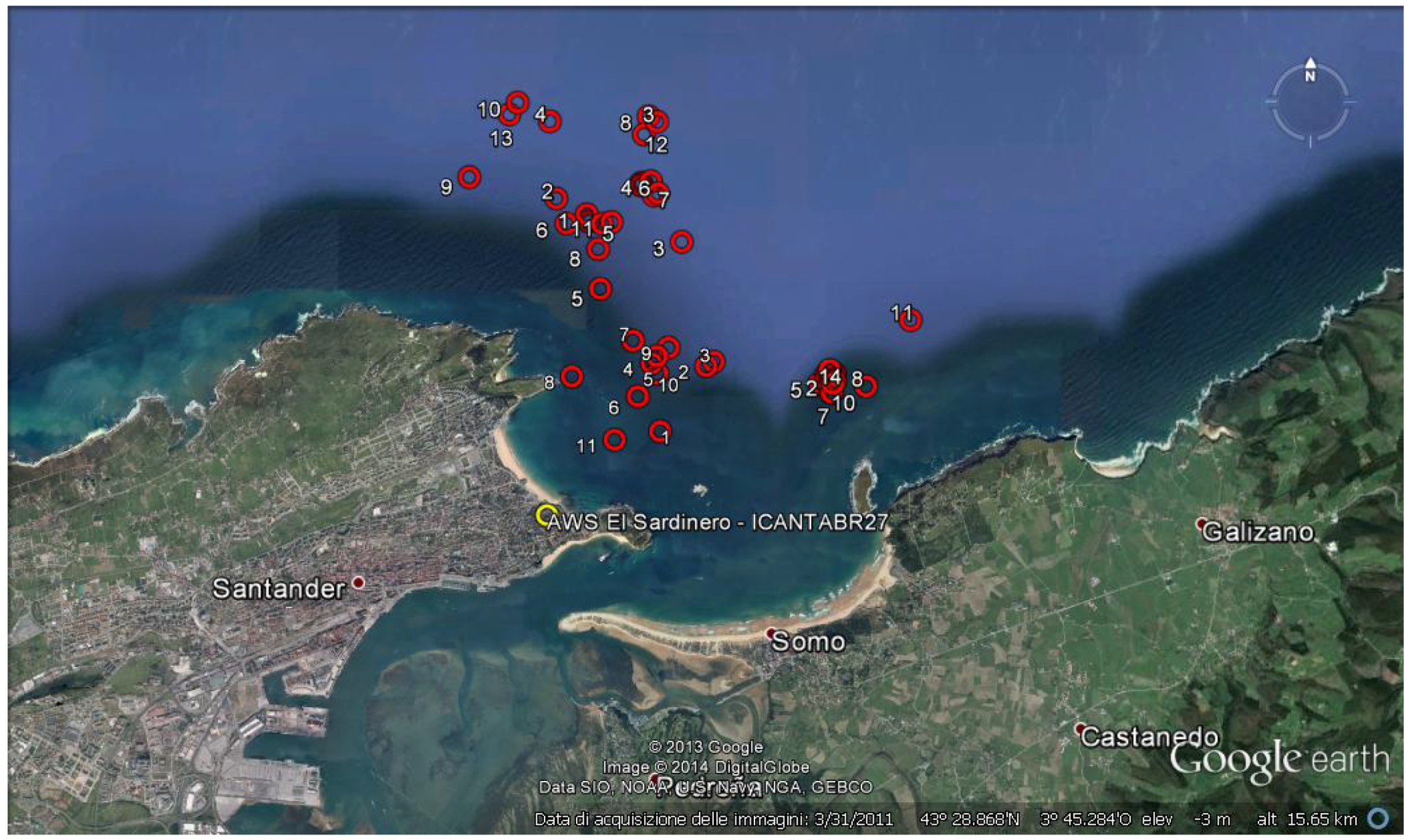
The meteorological data have been integrated with the measurements of the geographic coordinates (latitude and longitude) carried out with a GARMIN Forerunner 910XT [33] used in automatic registration modality in order to simplify the off-shore observation procedure. The off‑shore measuring points are shown in Figure 3.

Figure 3. Off-shore weather observations (red circles) made in the period September 8–15, 2013 and position of the Automatic Weather Station ICANTABR27 (yellow circle). The white numbers next to red circles represent the order of the measures for each day (some numbers are repeated because the measures were made on different days).

Figure 3. Off-shore weather observations (red circles) made in the period September 8–15, 2013 and position of the Automatic Weather Station ICANTABR27 (yellow circle). The white numbers next to red circles represent the order of the measures for each day (some numbers are repeated because the measures were made on different days).

2.3. Methods

2.3.1. Weather Patterns

By means of the WindRose PRO3 software and of the wind data measured by the Automatic Weather Station ICANTABR27 during the period September 8–21 of the years 2005–2013, and averaged over 1 h, the recurrent WPs of the regatta area have been determined. The reason for considering only the measurements of the month of September is that the Sailing World Championships was held in September 2014.

Wind speed and wind direction measured at the ICANTABR27 meteorological station have been associated, in two different charts, to air temperature and atmospheric pressure. In such way the relation between global and local atmospheric circulation conditions has been determined.

With the aim to differentiate between gradient wind (associated to the passage of fronts over the regatta area) and thermal wind (associated to land and sea breeze), the wind roses have been produced considering only two time intervals: 09:00 LT–13:00 LT and 14:00 LT–18:00 LT.

The resulting WPs have been used to evaluate the most frequent meteorological situations over the regatta field. Then, they have been compared to the WPs of the period September 8–15, 2013, and two of the latter have been selected because belonging to the most frequent WPs. These two cases have been analyzed to create the “Call Book”, which is the handy‑guide made available to athletes and coaches where the meteorological conditions and the relative strategic analysis are described in detail.

2.3.2. Comparison against the Observations

In order to judge the capability of the model to reproduce the meteorological fields, the CALMET results have been compared against the observations of the ICANTABR2 (or El Sardinero) meteorological station, which is located close to the shoreline (see Figure 2). Obviously the ICANTABR2 observations have not been used among the inputs of the CALMET model. The modeled data have been extracted for the whole time period (September 8–15, 2013) from the CALMET cell containing the El Sardinero station, then they have been compared against the observations for the daily period of interest, which runs from 9 to 18.

The original data measured from the El Sardinero meteorological station are available every 15 min. In order to be compared with the CALMET output, which are hourly averages, they have been averaged over one hour so that all the observations between hour K-1 and hour K determine the average of hour K.

A quantitative assessment of the agreement between modeled values and observations has been carried out by means of three statistics: the Normalized Mean BIAS (NMBIAS) to get information about over‑prediction or under‑prediction, the Mean Absolute Error (MAE) to get information about the absolute distance between observations and model results, and the Pearson Correlation Coefficient (PCC) to get information about the agreement of the time variation of observations and modeled values. The three statistics are defined as ([34,35,36]):

$$NMBIAS=100\frac{1}{n}{\displaystyle \sum _{k=1}^n\frac{p_k-o_k}{o_k}}$$

(1)

$$MAE=\frac{1}{n}{\displaystyle \sum _{k=1}^n\left|p_k-o_k\right|}$$

(2)

$$PCC=\frac{{\displaystyle \sum _{k=1}^n\left(p_k-p_{avg}\right)\left(o_k-o_{avg}\right)}}{\sqrt{{\displaystyle \sum _{k=1}^n{\left(p_k-p_{avg}\right)}^2}}\sqrt{{\displaystyle \sum _{k=1}^n{\left(o_k-o_{avg}\right)}^2}}}$$

(3)

where n is the number of observations (and predictions), p_k is the k-th modeled value and o_k is the corresponding k-th observed value, p_avg and o_avg are respectively the averages of modeled values and observations over a specific time period. Concerning the NMBIAS, a negative value indicates an under‑prediction, while a positive value indicates an over‑prediction; it has been multiplied by 100 in order to show the small values calculated for the temperature without using too much decimals. Of course NMBIAS = 0 does not necessarily indicate a perfect reproduction of the observations because the negative and the positive differences may be perfectly balanced. For this reason, the MAE is very useful, because it evaluates the absolute distance between modeled and observed values; MAE = 0 indicates a perfect agreement, but any other value of the MAE does not say anything about over- or under-predictions. The PCC values may be within the interval from −1 (complete counter correlation) to +1 (complete correlation). It is observed that, due to the presence of a numerical discontinuity for wind direction between 360 degrees and 1 degree (which are close directions even if numerically far), the brutal application of the PCC expression may give misleading results. For this reason, a surrogate of the PCC for the wind direction has been calculated by determining the components of the unit vector along the X and Y directions, calculating the PCC for each of such components independently, and then taking their average. The use of the unit vector assures that only the effect of wind direction is considered, not wind speed.

2.3.3. Use of the CALMET Results for Creating the “Call Book”

The “Call Book” must be a simple and easy-to-read tool, composed by images and brief descriptions of the meteorological situation and of the strategic analysis, tailored to be rapidly used by athletes and coaches. Examples of this type of meta‑communication and of the use of meteorological modeling for creating a “Call Book” have been developed by Houghton and Campbell [37] and Pezzoli [38].

The use of a limited scale meteorological model in hindcasting compensates for the lack of continuous measurements at sea, providing a distributed analysis of wind fields. The modeled data have been extracted for the whole time period (September 8–15, 2013) from the CALMET cells containing the points of the race area’s centers A, B, C, D, E (Figure 2). In such a way, a virtual database of meteorological variables to be analyzed with the WindRose PRO3 software has been built.

The analysis of these wind roses together with the measures made in the off-shore race area was made to build the “Call Book”. The meteorological data (wind direction, wind speed, air pressure and air temperature) was analyzed using a mobile average of the fifth order. It was chosen to use the mobile average instead of the instantaneous data because the mobile average helps to understand better the trend of the atmospheric pattern.

3. Results and Discussion

3.1. Weather Patterns

The ICANTABR27 wind data analyzed with the WindRose PRO3 software are illustrated in Figure 4 and Figure 5.

The two figures show that during the morning period the prevailing wind blows from the arc SSW-W, while during the afternoon period it blows from NE. This variation implies a prevailing thermal regime over the Santander bay with land breeze during the morning and sea breeze during the afternoon. On the other hand, the westerly wind, clearly of synoptic origin, remains almost constant, in terms of relative frequency, during the morning and the afternoon. For this reason, it is fundamental to evaluate how thermal wind and gradient wind interact generating the recurrent WPs. The multidimensional analysis described in Section 2.3.1 allows to generate the ternary plots shown in Figure 6 and Figure 7. In these two plots, the air temperature and the atmospheric pressure measured during the period 09:00–18:00 LT are represented by circles of different colors which are placed at a radial distance given by the wind speed, and at an angular coordinate given by the wind direction.

As illustrated in Figure 6 and Figure 7 the following WPs have been identified:

(1)

Wind from S-SSW. Pre-frontal situation (gradient from SSW), not frequent (5%), warm wind prevailing during the morning which rapidly rotates toward SW decreasing atmospheric pressure and increasing wind speed.

(2)

Wind from SW. Classic pre-frontal and frontal situation (gradient from SW), not frequent if analyzed alone (5%). Generally it is associated to pattern 3 since the atmospheric pressure rapidly increases as the front passes and wind rotates to W-NW. The wind from SW is stable until the passage of the front. The same pattern is presented by the land thermal from SW, which rotates to NE during the day (it is characterized by high atmospheric pressure and low wind intensity).

(3)

Wind from W-NW (intensity > 3–4 m/s). Classic and very frequent situation (30%). Characterized by wind rotation to the right till NW and its intensification during the day. The atmospheric pressure slightly increases during the day.

(4)

Wind from W-NW (intensity < 3–4 m/s). This transition situation is observed after the passage of the front and before the establishment of the high pressure conditions. It is quite frequent in the Santander bay (10%). The wind is highly variable in intensity and direction (it could even reach NNW). This is the case of September 9, 2013, which will be analyzed in detail in a following paragraph dedicated to the “Call Book”.

(5)

Wind from NE (sea breeze). Classic sea breeze situation, very frequent in the Santander bay (40%). The atmospheric pressure decreases during the day while the air temperature increases, therefore wind rotates to the right and increases its intensity. This is the case of September 13, 2013, which will be analyzed in detail in a following paragraph dedicated to the “Call Book”.

(6)

Wind from ENE (gradient wind). Possible gradient wind without any thermal effect, generated by a depression moving at south of Santander. Quite frequent in the Santander bay (10%), it may generate very intense winds with almost constant direction.

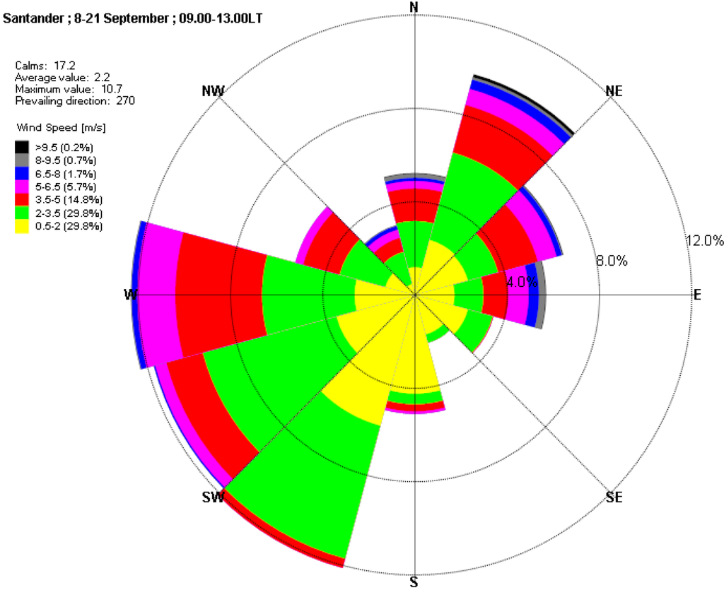
Figure 4. Wind rose for station ICANTABR27. Time interval 09.00 LT–13.00 LT, period September 8–21, years 2005–2013.

Figure 4. Wind rose for station ICANTABR27. Time interval 09.00 LT–13.00 LT, period September 8–21, years 2005–2013.

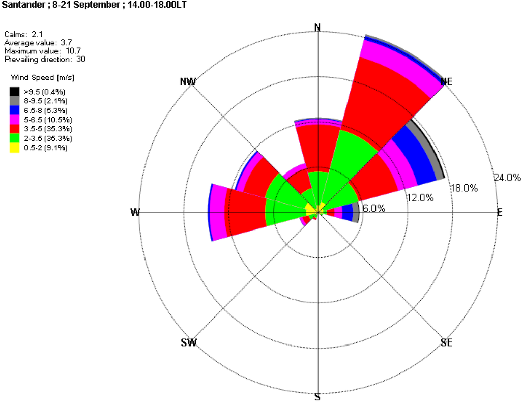
Figure 5. Wind rose for station ICANTABR27. Time interval 14.00 LT–18.00 LT, period September 8–21, years 2005–2013.

Figure 5. Wind rose for station ICANTABR27. Time interval 14.00 LT–18.00 LT, period September 8–21, years 2005–2013.

Figure 6. Ternary plot composed by wind speed (m/s), wind direction and air temperature (°C) observed by the ICANTABR27 station. Time interval 09.00 LT–18.00 LT, period September 8–21, years 2005–2013. The six WPs identified with the multidimensional analysis are represented over the plot.

Figure 6. Ternary plot composed by wind speed (m/s), wind direction and air temperature (°C) observed by the ICANTABR27 station. Time interval 09.00 LT–18.00 LT, period September 8–21, years 2005–2013. The six WPs identified with the multidimensional analysis are represented over the plot.

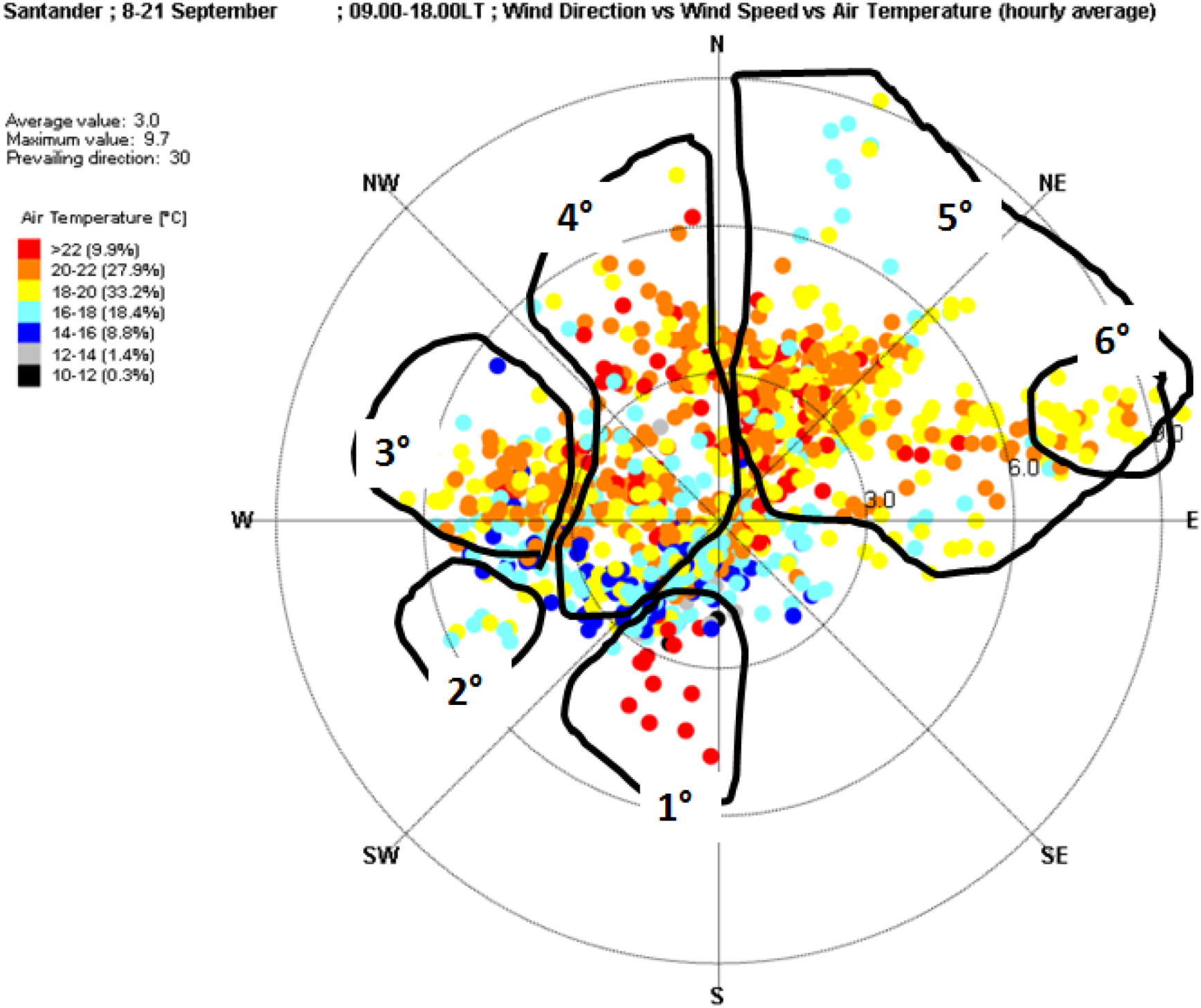
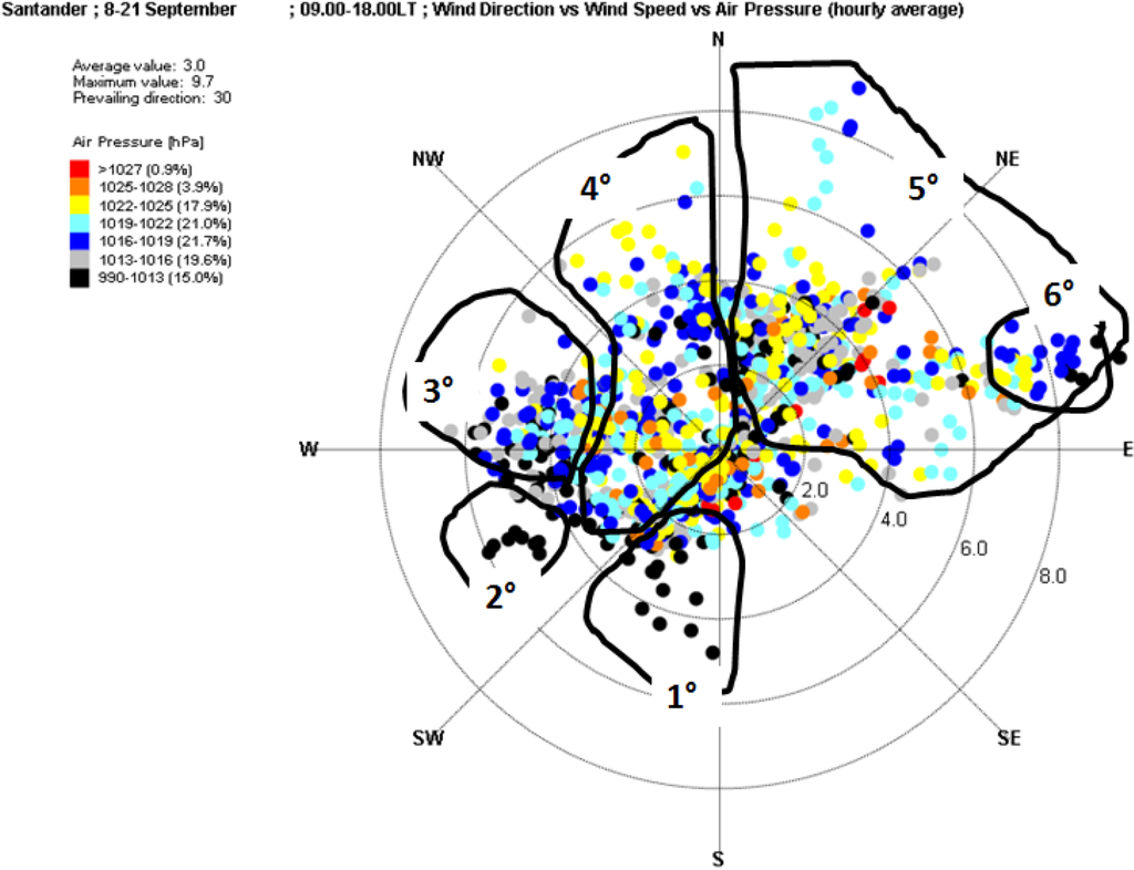
Figure 7. Ternary plot composed by wind speed (m/s), wind direction and atmospheric pressure (hPa) observed by the ICANTABR27. Time interval 09.00 LT–18.00 LT, period September 8–21, years 2005–2013.

Figure 7. Ternary plot composed by wind speed (m/s), wind direction and atmospheric pressure (hPa) observed by the ICANTABR27. Time interval 09.00 LT–18.00 LT, period September 8–21, years 2005–2013.

3.2. Comparison against the Observations

The observed and modeled wind roses at the El Sardinero station are represented in Figure 8, respectively in the left and right columns. The top row represents the wind roses obtained for the time period 09–13, and the bottom row represents the period 14–18.

A comparison of the time trends of observed and modeled values of wind direction, wind speed and temperature is shown in Figure 9 and Figure 10, respectively, for September 9 and 13, 2013. These two days have been chosen as examples among those simulated because:

• September 9 was characterized as a complex situation, due to the transition between gradient wind and thermal wind;
• September 13 was characterized by a pure thermal wind, with counterclockwise wind rotation from south west to north east and decreasing intensity between morning and afternoon, and almost constant wind direction and increased intensity during the afternoon.

Notwithstanding the two complex situations, CALMET is capable of reproducing the temporal variation of the meteorological variables in a satisfactory way, showing some differences between the morning and the afternoon. In particular, the wind direction is better reproduced during the afternoon than during the morning, probably because the meteorological situation is more stable in the afternoon, since the passage between land and sea breeze in Santander is between 12:00 and 13:00. The wind speed is slightly over-predicted during the afternoon and under-predicted during the morning, while the temperature is generally well predicted.

Figure 8. Observed (left column) and modeled (right column) wind roses at the El Sardinero station.

Figure 8. Observed (left column) and modeled (right column) wind roses at the El Sardinero station.

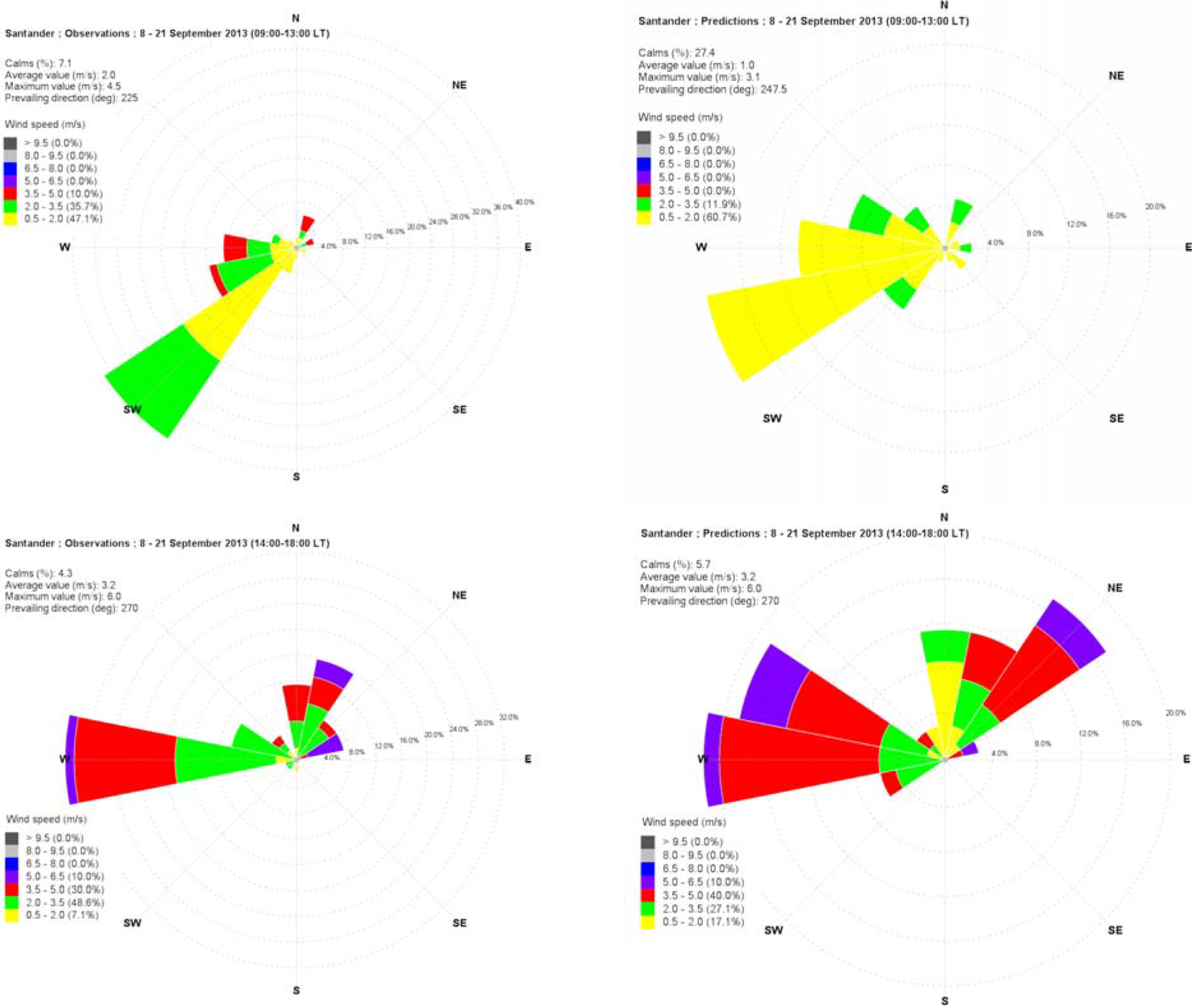
The numerical values of NMBIAS, MAE and PCC are reported in Table 1, Table 2 and Table 3, respectively. All the tables contain information for the morning (09–13) and for the afternoon (14–18) of all the simulated days.

The values of the NMBIAS show that wind direction and temperature are almost equally distributed between under- and over-predictions. On the contrary, the wind speed is always under‑predicted during the morning.

It can be observed that the average MAE values for atmospheric temperature are about 0.5–0.6 °C, and the average MAE values for wind speed are not greater than 1 m/s for the two time periods. On the contrary, the average MAE values for wind direction show a time variability: 30 degrees for the morning and 15 degrees for the afternoon. The MAE values are in any case good, demonstrating the ability of the CALMET model to reproduce the meteorological data observed by the El Sardinero station which was not used among its input.

Finally, the PCC values indicate a generally good agreement between the time variation of observations and of model results. The values 0.1, 0.3, 0.5 and 0.7 [39,40] may be used as thresholds to judge the correlations respectively as small, medium, large and very large. In order to simplify the analysis in this work, only two threshold values will be used: 0.3 and 0.7. A PCC value between 0 and 0.3 may be judged as a weak correlation, a PCC value between 0.3 and 0.7 may be judged as a moderate correlation, and PCC>0.7 is a strong correlation. A negative value of the PCC does not necessarily mean that the observations and the modeled results are very different from a numerical point of view, it means that they are varying in a different way with respect to the time. For example, PCC = −0.12 for wind direction during the morning of September 9, 2013, and Figure 9 shows that the values are numerically similar, but they are varying in a different manner from 11–12 LT: observed wind direction veering (i.e., rotating clockwise) while modeled wind direction backing (i.e., rotating counter clockwise).

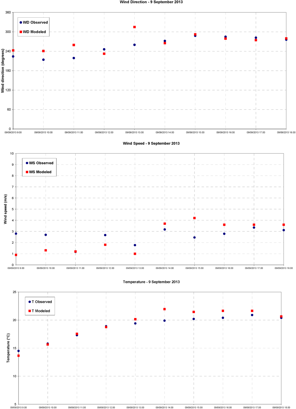
Figure 9. Comparison between observed (blue circles) and modeled (red squares) values of wind direction, wind speed and temperature at the El Sardinero station during the day of September 9, 2013.

Figure 9. Comparison between observed (blue circles) and modeled (red squares) values of wind direction, wind speed and temperature at the El Sardinero station during the day of September 9, 2013.

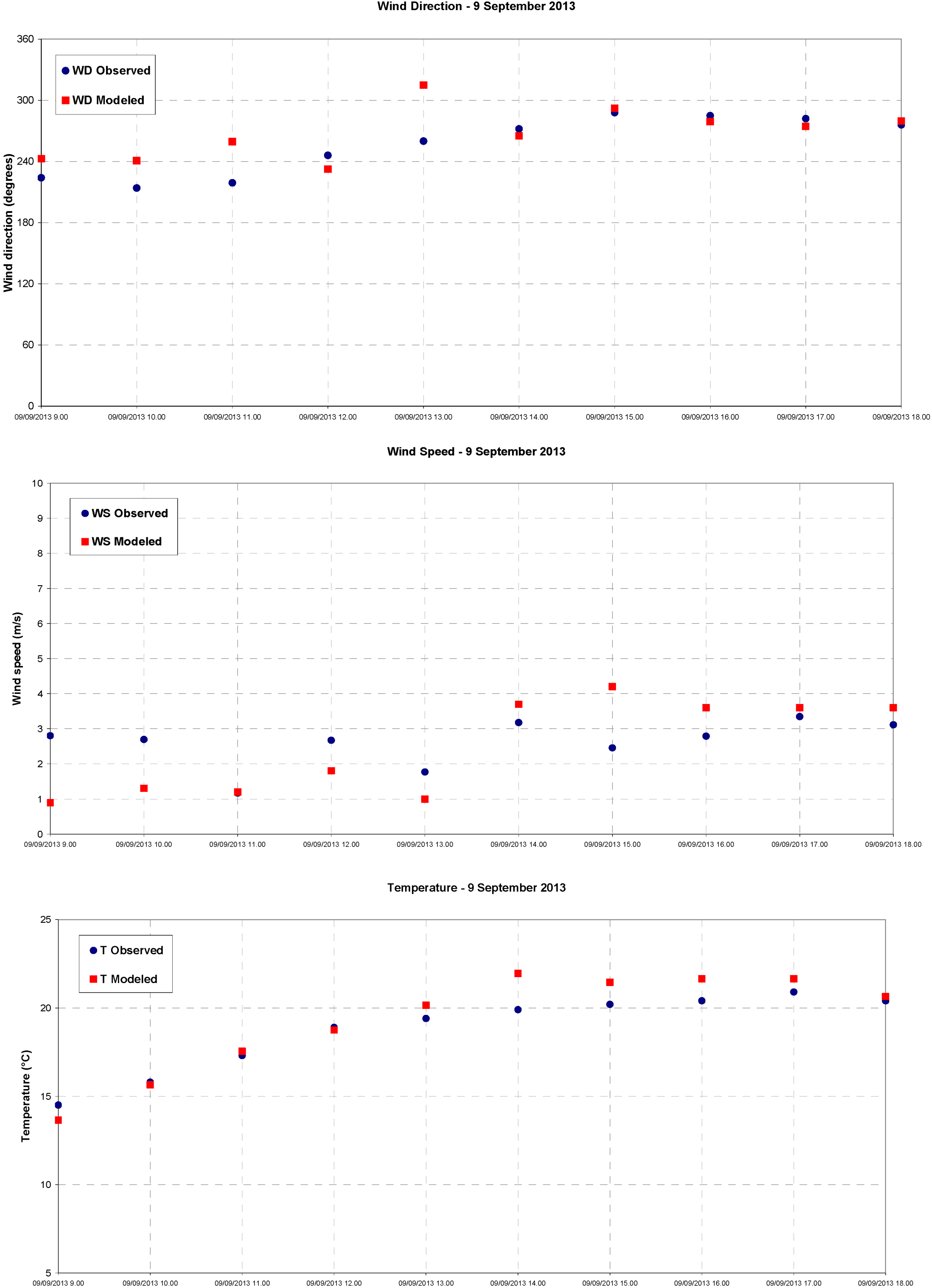
Figure 10. Comparison between observed (blue circles) and modeled (red squares) values of wind direction, wind speed and temperature at the El Sardinero station during the day of September 13, 2013.

Figure 10. Comparison between observed (blue circles) and modeled (red squares) values of wind direction, wind speed and temperature at the El Sardinero station during the day of September 13, 2013.

Summarizing, the CALMET results extracted at the grid point of the ICANTRBR2 station and compared with the observations of the station itself show that the model is capable of reconstructing the wind data. Since the predictions are in good agreement with the observations, the model results can be used to analyze wind patterns on the off-shore racing fields that can be easily utilized by the coaches and the athletes to decide the race strategy.

Therefore, CALMET can be used to rebuild the wind field within the race course and to create a virtual database for defining the “Call Book”.

Table 1. NMBIAS values calculated for all the days of analysis and for two different daily periods: 09–13 and 14–18. (WD: Wind Direction; WS: Wind Speed; T: Temperature).

Date	09–13			14–18
	WD	WS	T	WD	WS	T
08/09/2013	18.7	−5.0	−3.2	9.2	−44.5	2.5
09/09/2013	10.9	−44.2	−0.2	−0.9	25.7	5.5
10/09/2013	−5.8	−48.4	−2.6	9.1	−37.2	−1.0
11/09/2013	9.0	−42.4	−0.3	2.4	−1.7	0.8
12/09/2013	−2.0	−80.8	1.0	5.1	−33.5	5.8
13/09/2013	−2.2	−38.3	0.7	21.9	29.4	5.0
14/09/2013	7.2	−34.9	−1.6	2.2	2.9	2.7
15/09/2013	12.6	−43.8	−2.2	51.8	−34.7	1.1
16/09/2013	5.2	−48.6	−4.8	−6.6	−1.9	−1.0
17/09/2013	9.3	−37.9	−1.8	1.2	20.6	1.4
18/09/2013	10.7	−52.8	0.8	5.2	19.6	2.3
19/09/2013	18.7	−59.2	−2.7	−1.2	24.8	0.9
20/09/2013	6.8	−37.5	−0.3	12.8	−10.9	1.9
21/09/2013	−26.5	−39.0	−0.5	−13.6	−6.4	7.6
Minimum	−26.5	−80.8	−4.8	−13.6	−44.5	−1.0
Maximum	18.7	−5.0	1.0	51.8	29.4	7.6
Average	5.2	−43.8	−1.3	7.1	−3.4	2.5
Std. Dev.	11.6	16.3	1.7	15.4	25.8	2.6

Table 1. NMBIAS values calculated for all the days of analysis and for two different daily periods: 09–13 and 14–18. (WD: Wind Direction; WS: Wind Speed; T: Temperature).

Date	09–13			14–18
	WD	WS	T	WD	WS	T
08/09/2013	18.7	−5.0	−3.2	9.2	−44.5	2.5
09/09/2013	10.9	−44.2	−0.2	−0.9	25.7	5.5
10/09/2013	−5.8	−48.4	−2.6	9.1	−37.2	−1.0
11/09/2013	9.0	−42.4	−0.3	2.4	−1.7	0.8
12/09/2013	−2.0	−80.8	1.0	5.1	−33.5	5.8
13/09/2013	−2.2	−38.3	0.7	21.9	29.4	5.0
14/09/2013	7.2	−34.9	−1.6	2.2	2.9	2.7
15/09/2013	12.6	−43.8	−2.2	51.8	−34.7	1.1
16/09/2013	5.2	−48.6	−4.8	−6.6	−1.9	−1.0
17/09/2013	9.3	−37.9	−1.8	1.2	20.6	1.4
18/09/2013	10.7	−52.8	0.8	5.2	19.6	2.3
19/09/2013	18.7	−59.2	−2.7	−1.2	24.8	0.9
20/09/2013	6.8	−37.5	−0.3	12.8	−10.9	1.9
21/09/2013	−26.5	−39.0	−0.5	−13.6	−6.4	7.6
Minimum	−26.5	−80.8	−4.8	−13.6	−44.5	−1.0
Maximum	18.7	−5.0	1.0	51.8	29.4	7.6
Average	5.2	−43.8	−1.3	7.1	−3.4	2.5
Std. Dev.	11.6	16.3	1.7	15.4	25.8	2.6

Table 2. MAE values calculated for all the days of analysis and for two different daily periods: 09–13 and 14–18. (WD: Wind Direction; WS: Wind Speed; T: Temperature).

Date	09–13			14–18
	WD	WS	T	WD	WS	T
08/09/2013	53.5	0.7	0.7	14.0	1.5	0.6
09/09/2013	30.8	1.0	0.4	5.7	0.8	1.1
10/09/2013	15.1	1.3	0.5	52.9	0.8	0.4
11/09/2013	41.1	0.6	0.4	5.3	1.1	0.3
12/09/2013	19.2	1.4	0.4	14.7	1.2	1.1
13/09/2013	27.5	0.9	0.6	7.9	1.0	1.0
14/09/2013	16.8	0.8	0.3	7.3	0.4	0.6
15/09/2013	34.9	0.5	0.4	13.4	0.9	0.4
16/09/2013	15.6	1.4	0.8	23.3	0.7	0.4
17/09/2013	24.2	1.2	0.5	4.4	0.8	0.3
18/09/2013	26.2	1.7	0.5	14.1	0.9	0.6
19/09/2013	42.2	0.9	0.5	8.4	0.7	0.2
20/09/2013	19.1	0.7	0.3	31.7	0.6	0.4
21/09/2013	51.3	0.6	1.2	10.6	0.6	1.5
Minimum	15.1	0.5	0.3	4.4	0.4	0.2
Maximum	53.5	1.7	1.2	52.9	1.5	1.5
Average	29.8	1.0	0.5	15.3	0.8	0.6
Std. Dev.	13.0	0.4	0.2	13.2	0.3	0.4

Table 2. MAE values calculated for all the days of analysis and for two different daily periods: 09–13 and 14–18. (WD: Wind Direction; WS: Wind Speed; T: Temperature).

Date	09–13			14–18
	WD	WS	T	WD	WS	T
08/09/2013	53.5	0.7	0.7	14.0	1.5	0.6
09/09/2013	30.8	1.0	0.4	5.7	0.8	1.1
10/09/2013	15.1	1.3	0.5	52.9	0.8	0.4
11/09/2013	41.1	0.6	0.4	5.3	1.1	0.3
12/09/2013	19.2	1.4	0.4	14.7	1.2	1.1
13/09/2013	27.5	0.9	0.6	7.9	1.0	1.0
14/09/2013	16.8	0.8	0.3	7.3	0.4	0.6
15/09/2013	34.9	0.5	0.4	13.4	0.9	0.4
16/09/2013	15.6	1.4	0.8	23.3	0.7	0.4
17/09/2013	24.2	1.2	0.5	4.4	0.8	0.3
18/09/2013	26.2	1.7	0.5	14.1	0.9	0.6
19/09/2013	42.2	0.9	0.5	8.4	0.7	0.2
20/09/2013	19.1	0.7	0.3	31.7	0.6	0.4
21/09/2013	51.3	0.6	1.2	10.6	0.6	1.5
Minimum	15.1	0.5	0.3	4.4	0.4	0.2
Maximum	53.5	1.7	1.2	52.9	1.5	1.5
Average	29.8	1.0	0.5	15.3	0.8	0.6
Std. Dev.	13.0	0.4	0.2	13.2	0.3	0.4

Table 3. PCC values calculated for all the days of analysis and for three different daily periods: 09–13 and 14–18. (WD: Wind Direction; WS: Wind Speed; T: Temperature).

Date	09–13			14–18
	WD	WS	T	WD	WS	T
08/09/2013	−0.23	−0.90	0.92	0.66	−0.74	0.88
09/09/2013	−0.12	0.23	0.99	0.75	−0.79	−0.20
10/09/2013	0.74	0.26	0.77	0.66	1.00	0.46
11/09/2013	0.58	0.63	0.96	0.75	0.35	0.90
12/09/2013	0.68	−0.55	0.99	0.74	0.67	−0.73
13/09/2013	0.71	−0.36	0.98	0.74	0.70	0.51
14/09/2013	0.71	0.63	0.98	0.74	0.41	0.66
15/09/2013	0.68	0.82	0.98	0.72	0.78	0.85
16/09/2013	0.67	0.44	0.99	0.73	0.60	0.61
17/09/2013	0.67	0.67	0.99	0.73	0.97	0.98
18/09/2013	0.66	0.63	0.95	0.73	0.87	0.03
19/09/2013	0.65	0.46	0.85	0.72	0.19	0.97
20/09/2013	0.66	0.81	0.99	0.69	0.65	0.85
21/09/2013	0.59	0.98	1.00	0.69	0.40	0.52
Minimum	−0.23	−0.90	0.77	0.66	−0.79	−0.73
Maximum	0.74	0.98	1.00	0.75	1.00	0.98
Average	0.55	0.34	0.95	0.72	0.43	0.52
Std. Dev.	0.31	0.56	0.07	0.03	0.56	0.50

Table 3. PCC values calculated for all the days of analysis and for three different daily periods: 09–13 and 14–18. (WD: Wind Direction; WS: Wind Speed; T: Temperature).

Date	09–13			14–18
	WD	WS	T	WD	WS	T
08/09/2013	−0.23	−0.90	0.92	0.66	−0.74	0.88
09/09/2013	−0.12	0.23	0.99	0.75	−0.79	−0.20
10/09/2013	0.74	0.26	0.77	0.66	1.00	0.46
11/09/2013	0.58	0.63	0.96	0.75	0.35	0.90
12/09/2013	0.68	−0.55	0.99	0.74	0.67	−0.73
13/09/2013	0.71	−0.36	0.98	0.74	0.70	0.51
14/09/2013	0.71	0.63	0.98	0.74	0.41	0.66
15/09/2013	0.68	0.82	0.98	0.72	0.78	0.85
16/09/2013	0.67	0.44	0.99	0.73	0.60	0.61
17/09/2013	0.67	0.67	0.99	0.73	0.97	0.98
18/09/2013	0.66	0.63	0.95	0.73	0.87	0.03
19/09/2013	0.65	0.46	0.85	0.72	0.19	0.97
20/09/2013	0.66	0.81	0.99	0.69	0.65	0.85
21/09/2013	0.59	0.98	1.00	0.69	0.40	0.52
Minimum	−0.23	−0.90	0.77	0.66	−0.79	−0.73
Maximum	0.74	0.98	1.00	0.75	1.00	0.98
Average	0.55	0.34	0.95	0.72	0.43	0.52
Std. Dev.	0.31	0.56	0.07	0.03	0.56	0.50

3.3. Use of the CALMET Results for Creating the “Call Book”

The wind roses for the period September 8–21, 2013 in the race area’s centers A, B, C, D and E are illustrated in Figure 11, Figure 12, Figure 13, Figure 14, Figure 15, Figure 16, Figure 17, Figure 18, Figure 19 and Figure 20.

Figure 11. Wind rose for the race area A. Time interval 09:00 LT–13:00 LT, period September 8–21, 2013.

Figure 11. Wind rose for the race area A. Time interval 09:00 LT–13:00 LT, period September 8–21, 2013.

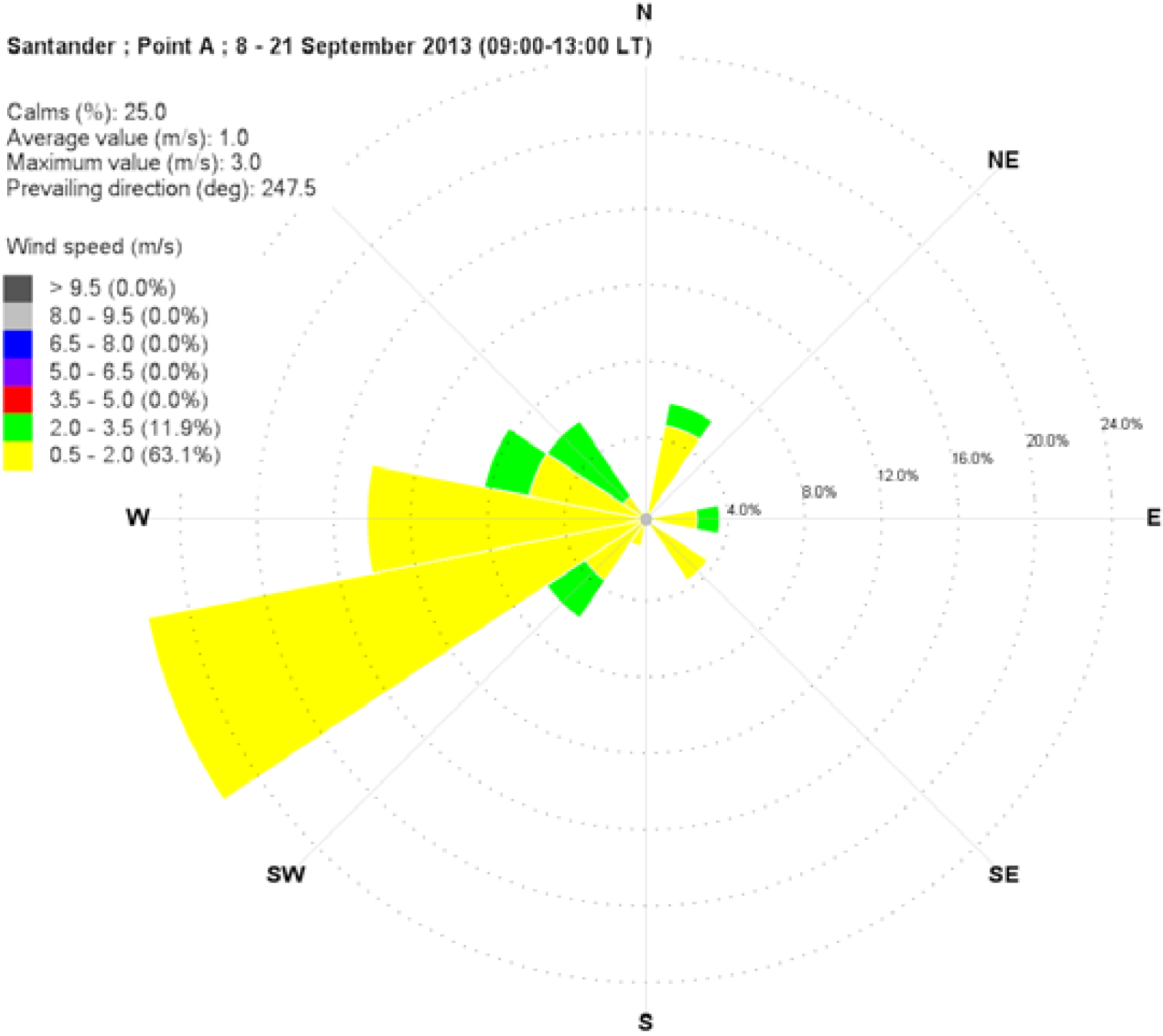
Figure 12. Wind rose for the race area A. Time interval 14:00 LT–18:00 LT, period September 8–21, 2013.

Figure 12. Wind rose for the race area A. Time interval 14:00 LT–18:00 LT, period September 8–21, 2013.

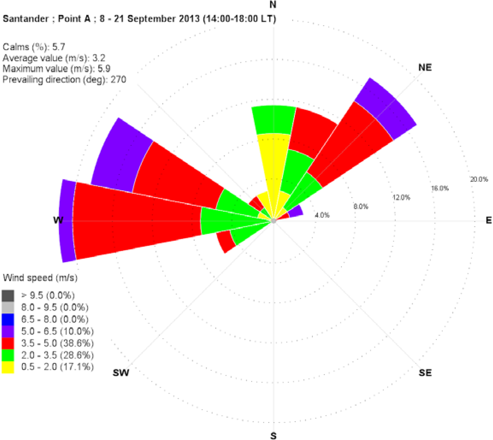
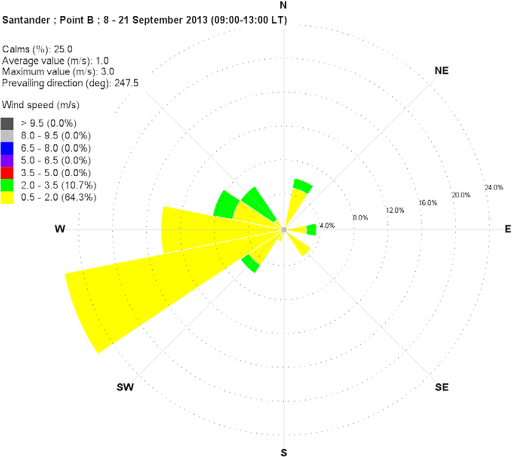
Figure 13. Wind rose for the race area B. Time interval 09:00 LT–13:00 LT, period September 8–21, 2013.

Figure 13. Wind rose for the race area B. Time interval 09:00 LT–13:00 LT, period September 8–21, 2013.

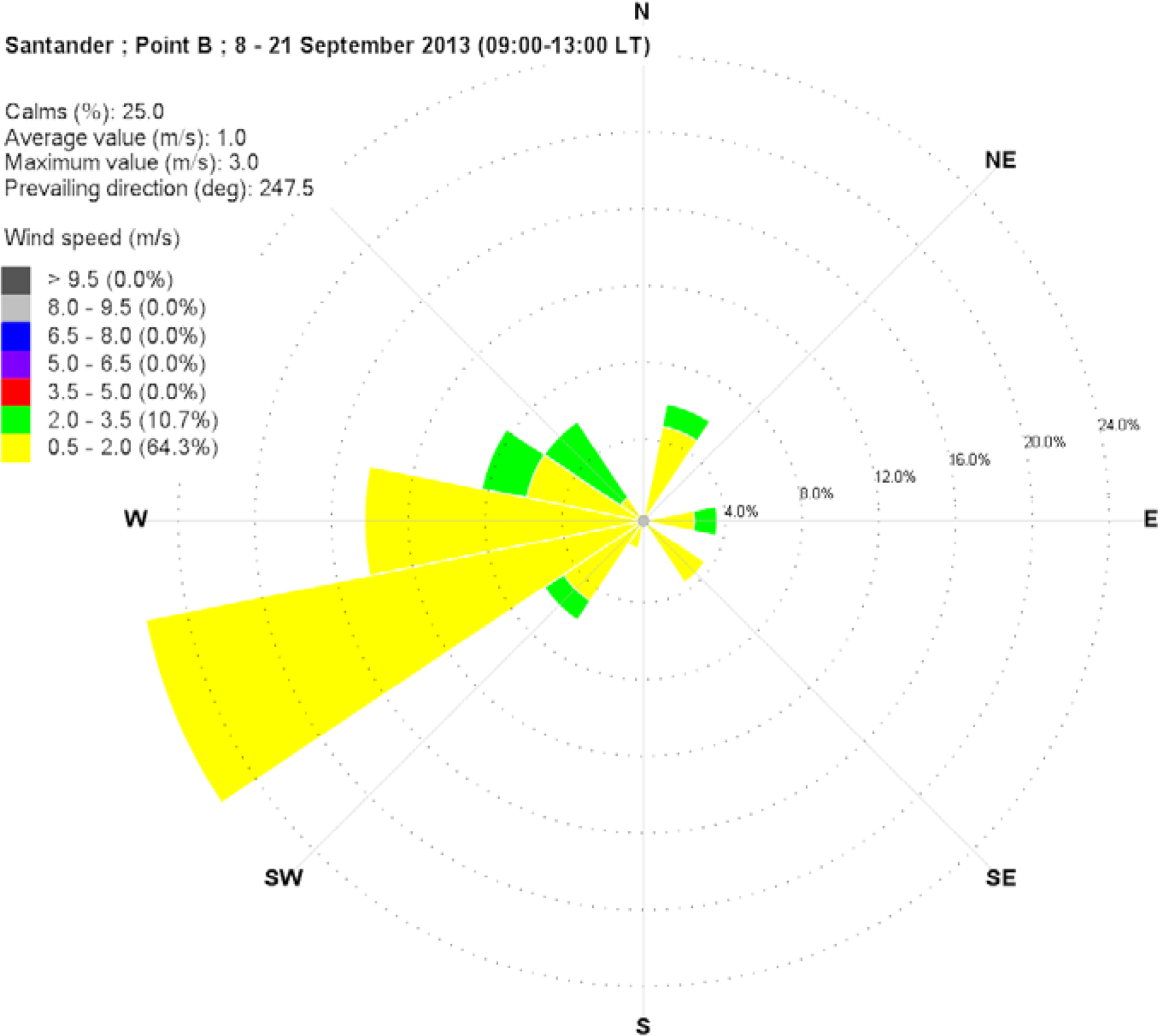
Figure 14. Wind rose for the race area B. Time interval 14:00 LT–18:00 LT, period September 8–21, 2013.

Figure 14. Wind rose for the race area B. Time interval 14:00 LT–18:00 LT, period September 8–21, 2013.

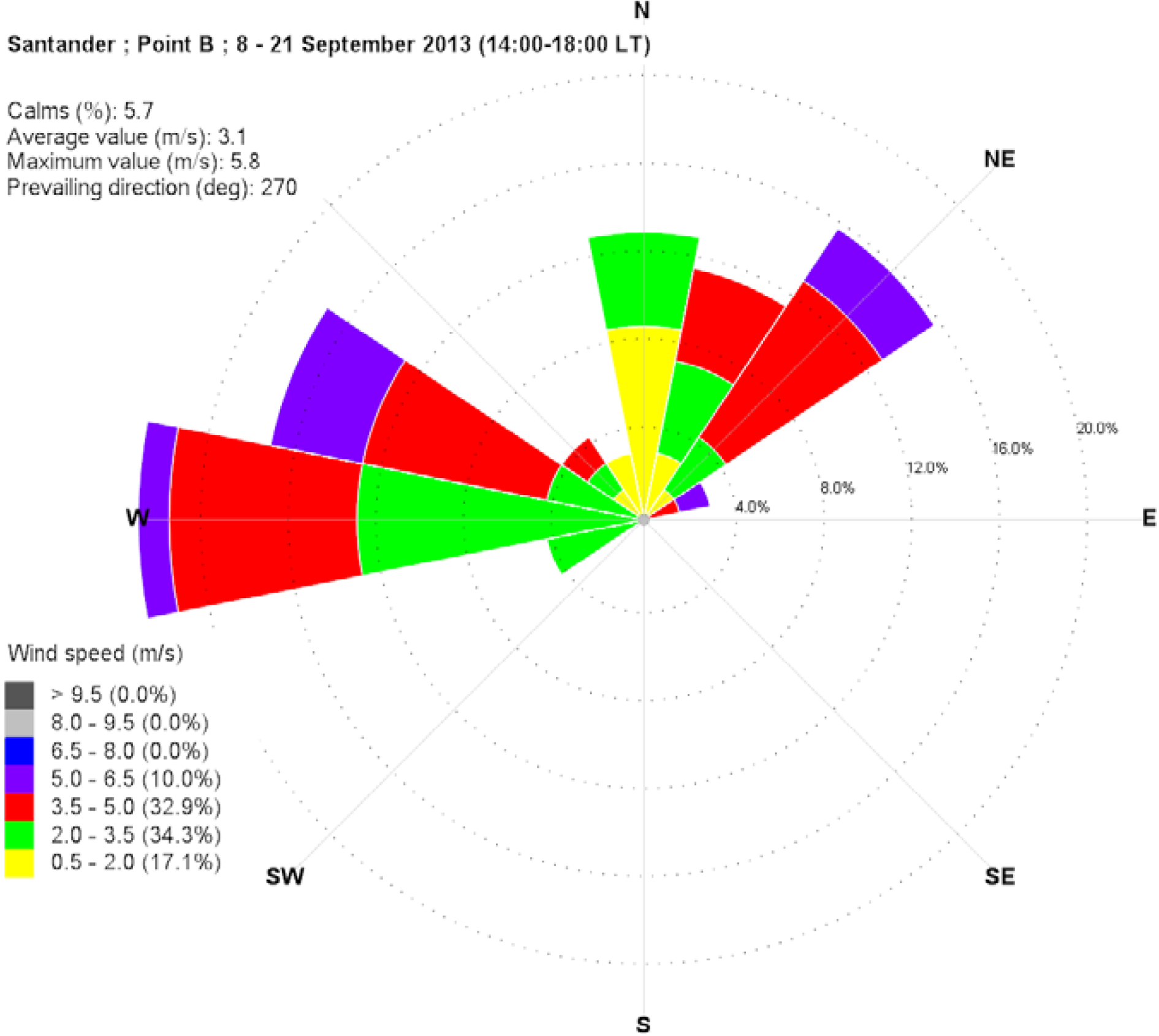
Figure 15. Wind rose for the race area C. Time interval 09:00 LT–13:00 LT, period September 8–21, 2013.

Figure 15. Wind rose for the race area C. Time interval 09:00 LT–13:00 LT, period September 8–21, 2013.

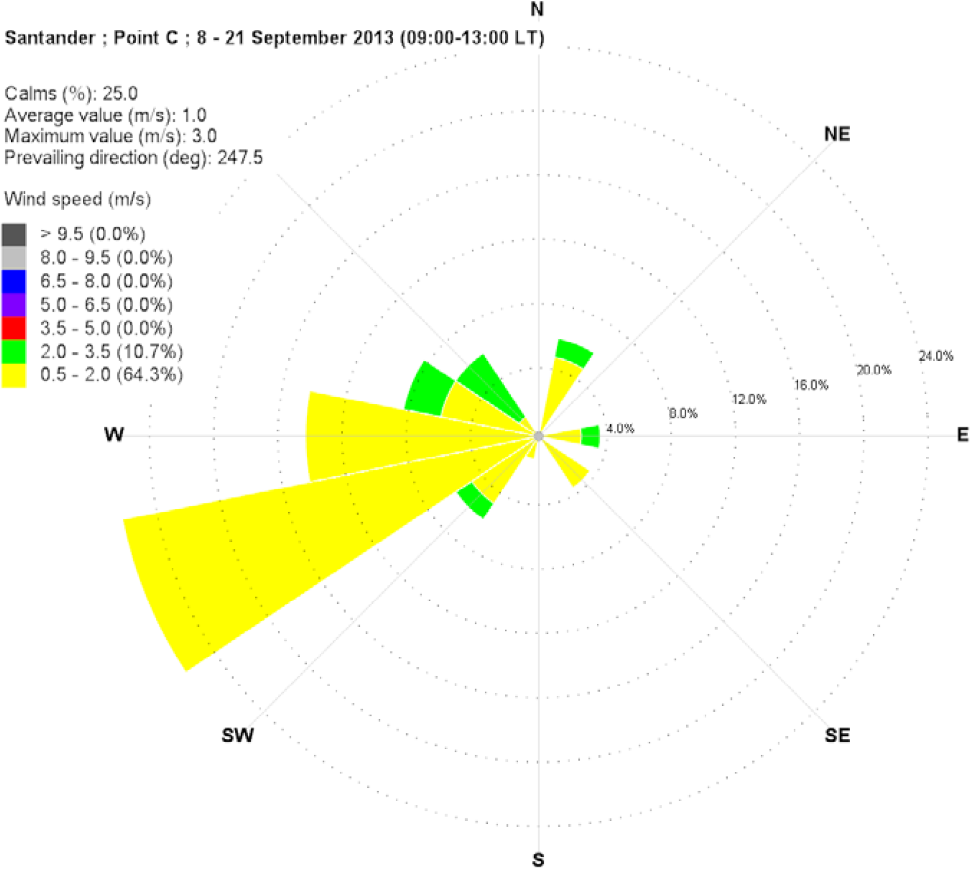
Figure 16. Wind rose for the race area C. Time interval 14:00 LT–18:00 LT, period September 8–21, 2013.

Figure 16. Wind rose for the race area C. Time interval 14:00 LT–18:00 LT, period September 8–21, 2013.

Figure 17. Wind rose for the race area D. Time interval 09:00 LT–13:00 LT, period September 8–21, 2013.

Figure 17. Wind rose for the race area D. Time interval 09:00 LT–13:00 LT, period September 8–21, 2013.

Figure 18. Wind rose for the race area D. Time interval 14:00 LT–18:00 LT, period September 8–21, 2013.

Figure 18. Wind rose for the race area D. Time interval 14:00 LT–18:00 LT, period September 8–21, 2013.

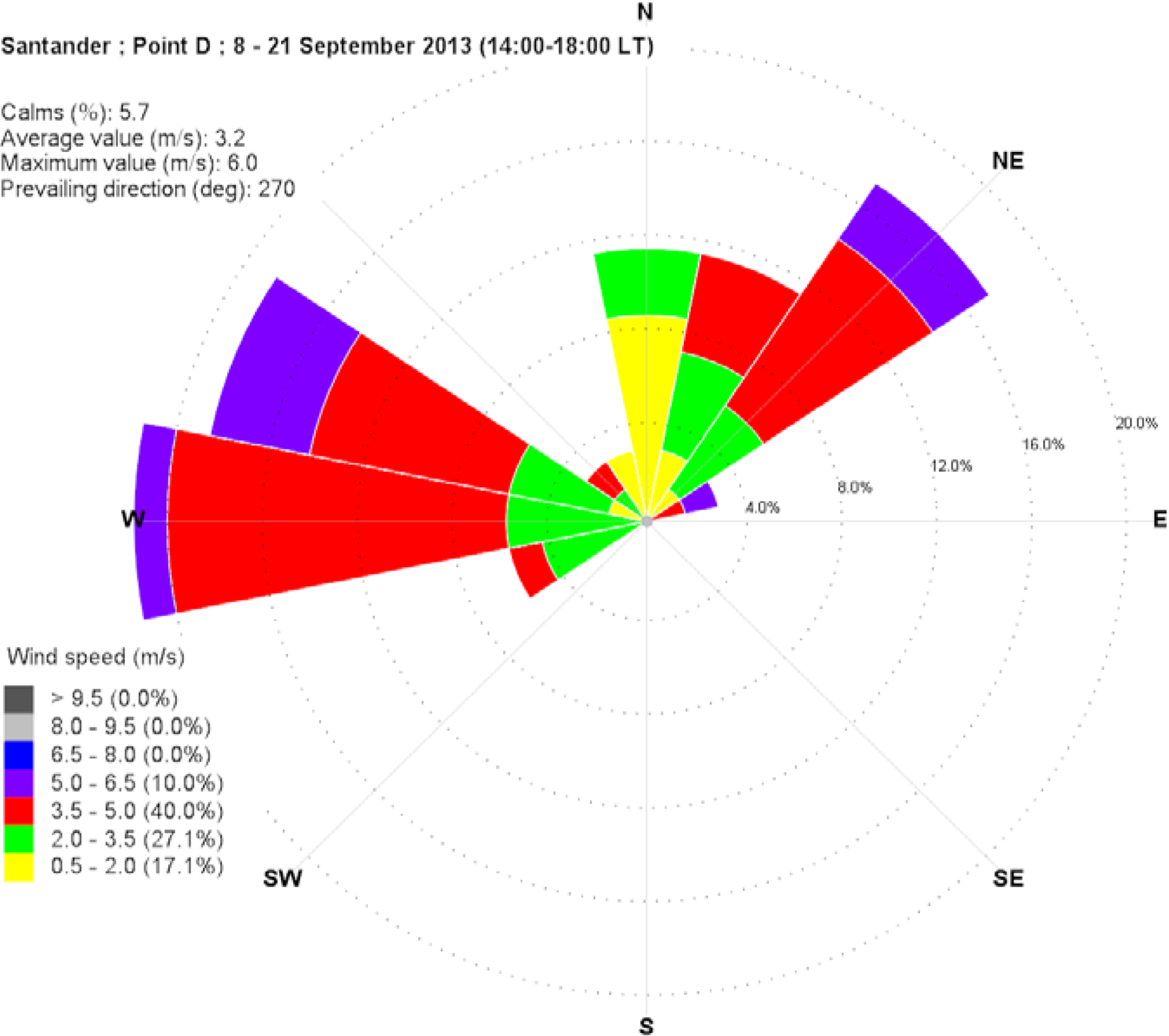
Figure 19. Wind rose for the race area E. Time interval 09:00 LT–13:00 LT, period September 8–21, 2013.

Figure 19. Wind rose for the race area E. Time interval 09:00 LT–13:00 LT, period September 8–21, 2013.

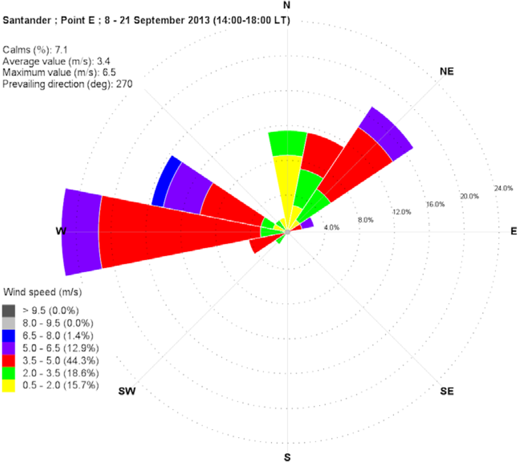
Figure 20. Wind rose for the race area E. Time interval 14:00 LT–18:00 LT, period September 8–21, 2013.

Figure 20. Wind rose for the race area E. Time interval 14:00 LT–18:00 LT, period September 8–21, 2013.

Keeping in mind Section 2.3.3 and observing Figure 11, Figure 12, Figure 13, Figure 14, Figure 15, Figure 16, Figure 17, Figure 18, Figure 19 and Figure 20, the race course of Santander may be classified as belonging to the third category (race course where the wind direction remains constant but varies in intensity). This information is of great interest to athletes and coaches because these kinds of regatta fields are very difficult as one may notice differences in strategies between two race courses (often very close to each other) even though the same wind directions and the same wind-shift are measured.

At the same time, observing Figure 15, Figure 16 and Figure 17, Figure 18, it can be noted that the wind roses of race area C and D are quite similar. This observation identifies a situation where the race courses close to the coastal line are very similar from a strategically point of view and they have an evident difference with the off-shore race fields.

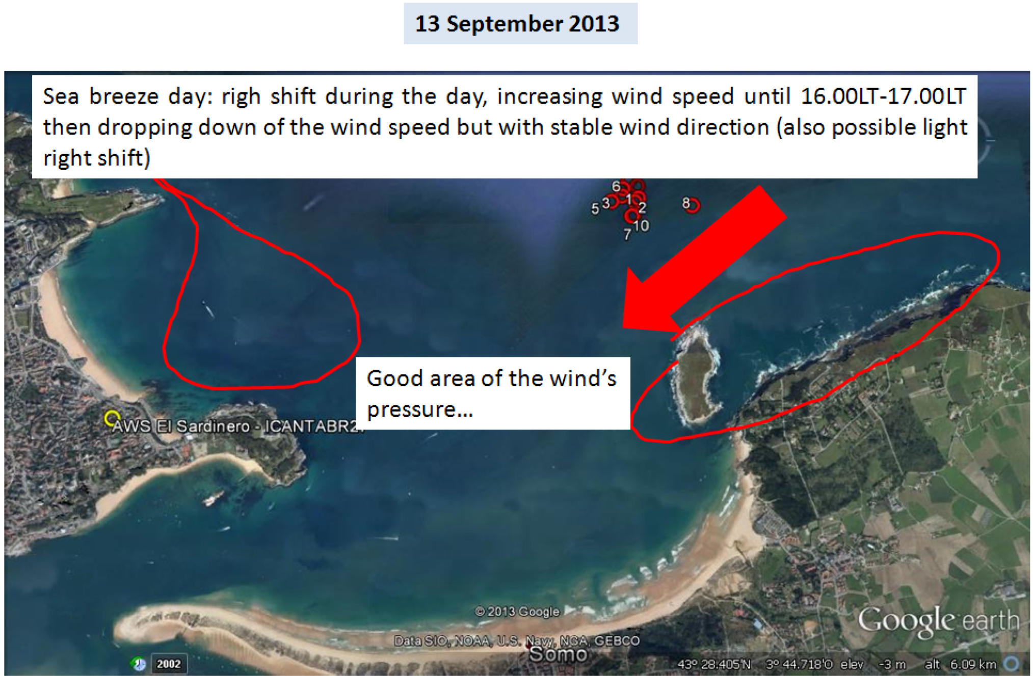
The analysis of what happened on September 13, 2013 (see also Figure 10) is a confirmation of these statements. On that day, one of the authors was on the race course C carrying out analysis and study for the Swedish Sailing Federation during the ISAF Test Event, at the same time other athletes were racing on the regatta field B. It was noted that in the two racing fields the situation was almost the same, but actually the races were conducted in different ways despite having measured the same wind direction on the two fields (and pretty much the same intensity). What happened? Why with the same NE wind in race field C did a boat have to go to the right (toward the coast) and in race field B, despite having received a right rotation did a boat have to go to the left? This behavior is well explained by the wind roses of the period 14–18 of points B and C (Figure 14 and Figure 16). What should a coach or an athlete expect from the analysis of these two wind roses? One should expect pretty much the same wind direction (and in fact there was), then one should also expect an intensification of the NE winds at point C with respect to point B, or an increase in frequency of higher intensities from NE for point C (and in fact that is noted observing the wind roses), and a wind more to the left (N-NNE most frequent) at point B (and in fact this phenomenon is illustrated by the wind roses).

This analysis confirms that, with the wind from NE, in the race fields close to the coast (C, D) it is necessary to go to the right to receive more wind pressure when the sea breeze is fully developed (these two fields require a strategically approach which prevails on tactic), while in the race field B it is suggested to keep checking the left together with the opponents (it is a field more tactic than strategic).

3.3.1. September 9, 2013

Figure 21 and Figure 22 show the modeled wind field over an extended portion of the simulation domain for September 9, 2013 at times 10:00 LT and 15:00 LT, respectively. At 10:00 LT, the modeled wind blows from south-west with speeds which are within the interval 1.3–1.5 m/s, while at 15:00 LT the wind blows from north‑west with speeds within the interval 2.1–5.1 m/s.

From this analysis, and from the analysis of the observations carried out in-situ (Figure 23, Figure 24 and Figure 25), it is possible to produce a description of the regatta field which, through an appropriate meta-communication, is able to provide a simplified representation of the race course. Figure 26 incorporates all the main suggestions and shows how the strategic evaluation of the race course is carried out in an extremely effective way.

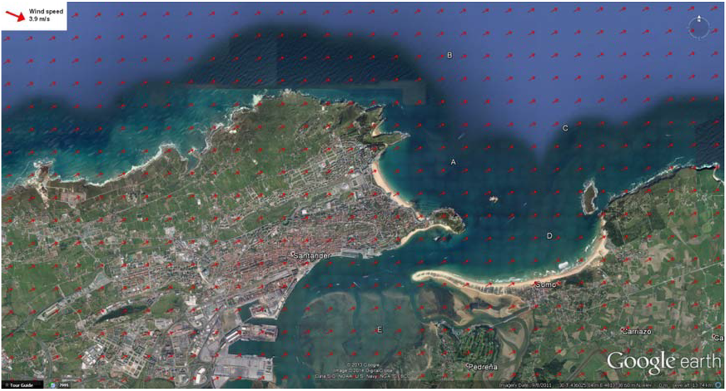
Figure 21. Modeled wind field over a portion of the simulation domain: September 9, 2013 at 10:00 LT. The red arrow in the upper left box represents the wind speed scale.

Figure 21. Modeled wind field over a portion of the simulation domain: September 9, 2013 at 10:00 LT. The red arrow in the upper left box represents the wind speed scale.

Figure 22. Modeled wind field over a portion of the simulation domain: September 9, 2013 at 15:00 LT. The red arrow in the upper left box represents the wind speed scale.

Figure 22. Modeled wind field over a portion of the simulation domain: September 9, 2013 at 15:00 LT. The red arrow in the upper left box represents the wind speed scale.

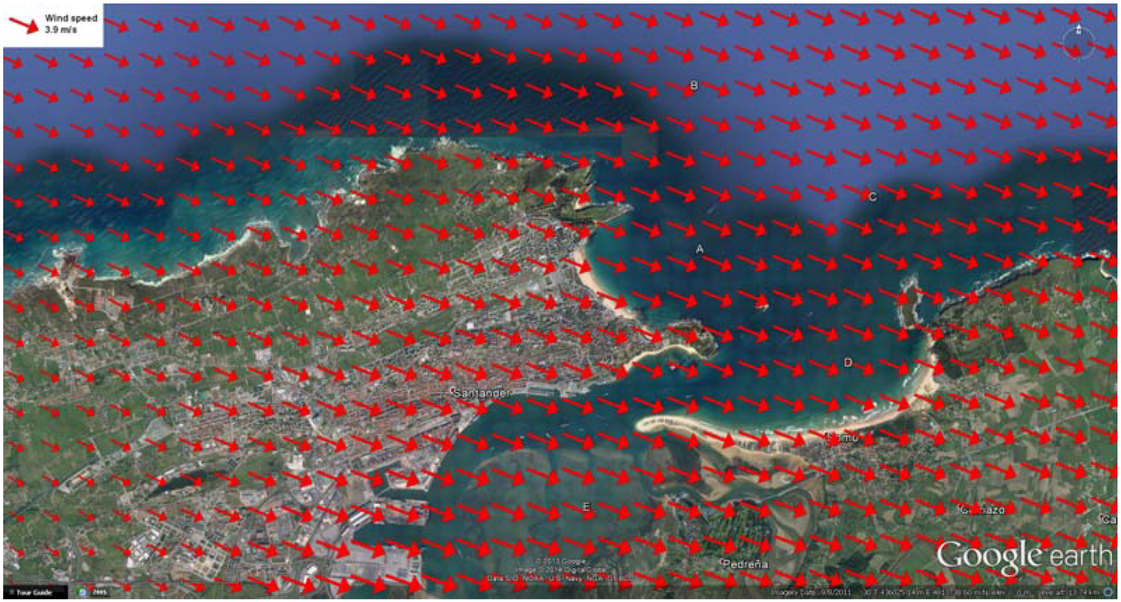
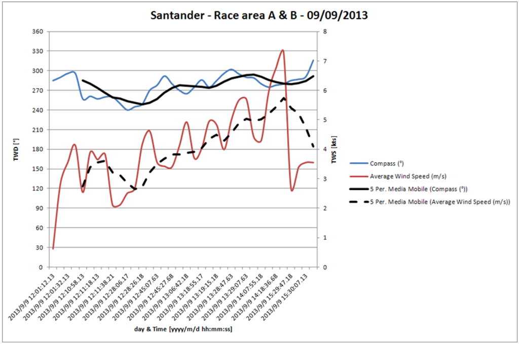
Figure 23. Wind direction (blue line) and speed (red line) measured over the regatta fields A and B on September 9, 2013. The moving average (factor 5) for wind direction (black solid line) and for wind speed (black dashed line) are also shown.

Figure 23. Wind direction (blue line) and speed (red line) measured over the regatta fields A and B on September 9, 2013. The moving average (factor 5) for wind direction (black solid line) and for wind speed (black dashed line) are also shown.

Figure 24. Wind direction (blue line) and speed (red line) measured by the ICANTABR27 station on September 9, 2013. The moving average (factor 5) for wind direction (black solid line) and for wind speed (black dashed line) are also shown.

Figure 24. Wind direction (blue line) and speed (red line) measured by the ICANTABR27 station on September 9, 2013. The moving average (factor 5) for wind direction (black solid line) and for wind speed (black dashed line) are also shown.

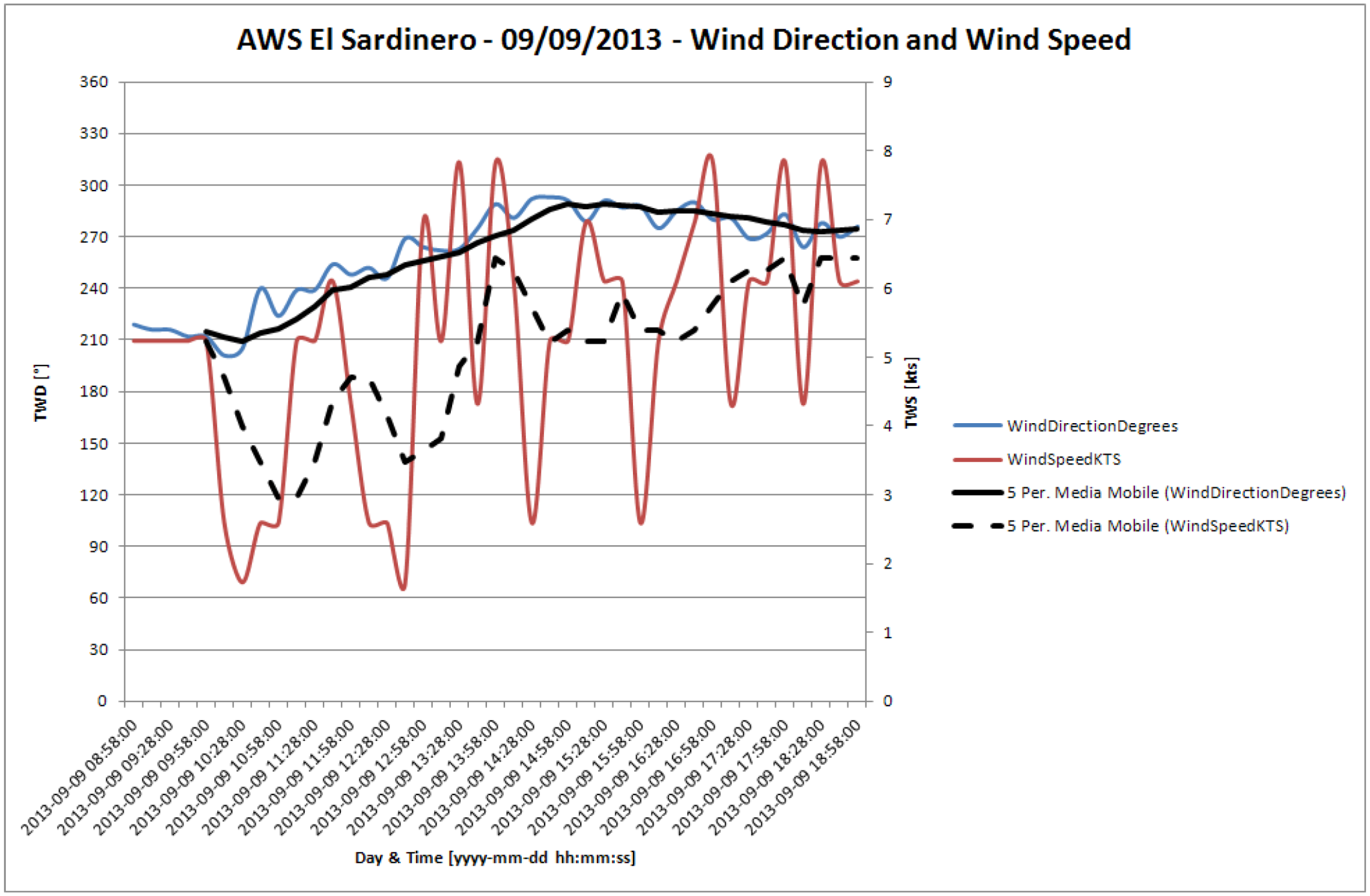
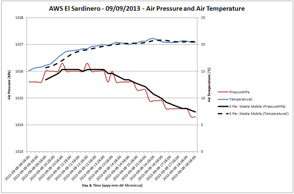
Figure 25. Air temperature (blue line) and atmospheric pressure (red line) measured by the ICANTABR27 station on September 9, 2013. The moving average (factor 5) for air temperature (black dashed line) and for wind speed (black solid line) are also shown.

Figure 25. Air temperature (blue line) and atmospheric pressure (red line) measured by the ICANTABR27 station on September 9, 2013. The moving average (factor 5) for air temperature (black dashed line) and for wind speed (black solid line) are also shown.

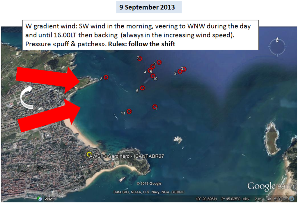
Figure 26. “Call book” for the situation characterized by gradient wind from W-NW over the race course. Transition from a regime of atmospheric depression and gradient wind to a thermal regime.

Figure 26. “Call book” for the situation characterized by gradient wind from W-NW over the race course. Transition from a regime of atmospheric depression and gradient wind to a thermal regime.

3.3.2. September 13, 2013

Figure 27 and Figure 28 show the modeled wind field over an extended portion of the simulation domain for September 13, 2013 at times 13:00 LT and 15:00 LT, respectively. At 13:00 LT, the modeled wind blows from east with speeds which are within the interval 1.3–1.6 m/s, while at 15:00 LT the wind blows from north‑east with speeds within the interval 4.4–4.7 m/s.

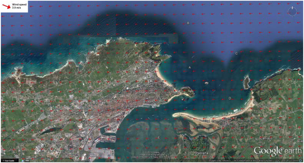
Figure 27. Modeled wind field over a portion of the simulation domain: September 13, 2013 at 13:00 LT. The red arrow in the upper left box represents the wind speed scale.

Figure 27. Modeled wind field over a portion of the simulation domain: September 13, 2013 at 13:00 LT. The red arrow in the upper left box represents the wind speed scale.

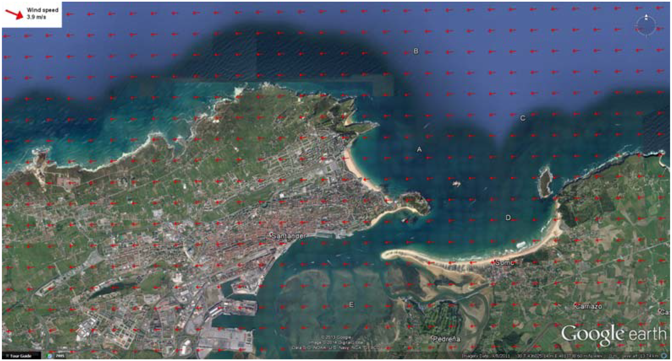
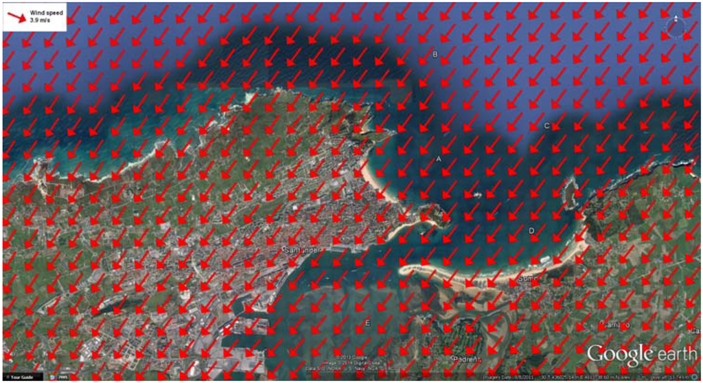
Figure 28. Modeled wind field over a portion of the simulation domain: September 13, 2013 at 15:00 LT. The red arrow in the upper left box represents the wind speed scale.

Figure 28. Modeled wind field over a portion of the simulation domain: September 13, 2013 at 15:00 LT. The red arrow in the upper left box represents the wind speed scale.

The in-situ measurements (Figure 29, Figure 30 and Figure 31) allowed to create a strategic analysis of the regatta field, which constitutes part of the “Call Book”. Figure 32 allows generalizing the strategic evaluation of the race course for all the “Sea Breeze” cases associated with null or weak gradient wind from SW.

Figure 29. Wind direction (blue line) and speed (red line) measured over the regatta fields A and B on September 13, 2013. The moving average (factor 5) for wind direction (black solid line) and for wind speed (black dashed line) are also shown.

Figure 29. Wind direction (blue line) and speed (red line) measured over the regatta fields A and B on September 13, 2013. The moving average (factor 5) for wind direction (black solid line) and for wind speed (black dashed line) are also shown.

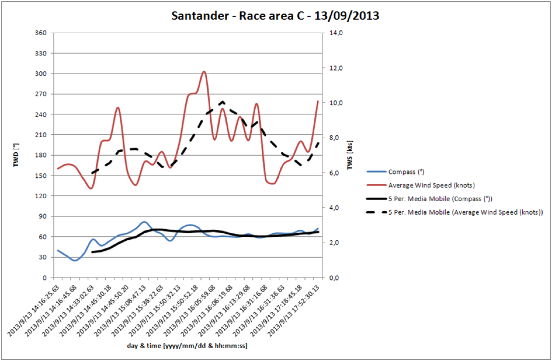
Figure 30. Wind direction (blue line) and speed (red line) measured by the ICANTABR27 station on September 13, 2013. The moving average (factor 5) for wind direction (black solid line) and for wind speed (black dashed line) are also shown.

Figure 30. Wind direction (blue line) and speed (red line) measured by the ICANTABR27 station on September 13, 2013. The moving average (factor 5) for wind direction (black solid line) and for wind speed (black dashed line) are also shown.

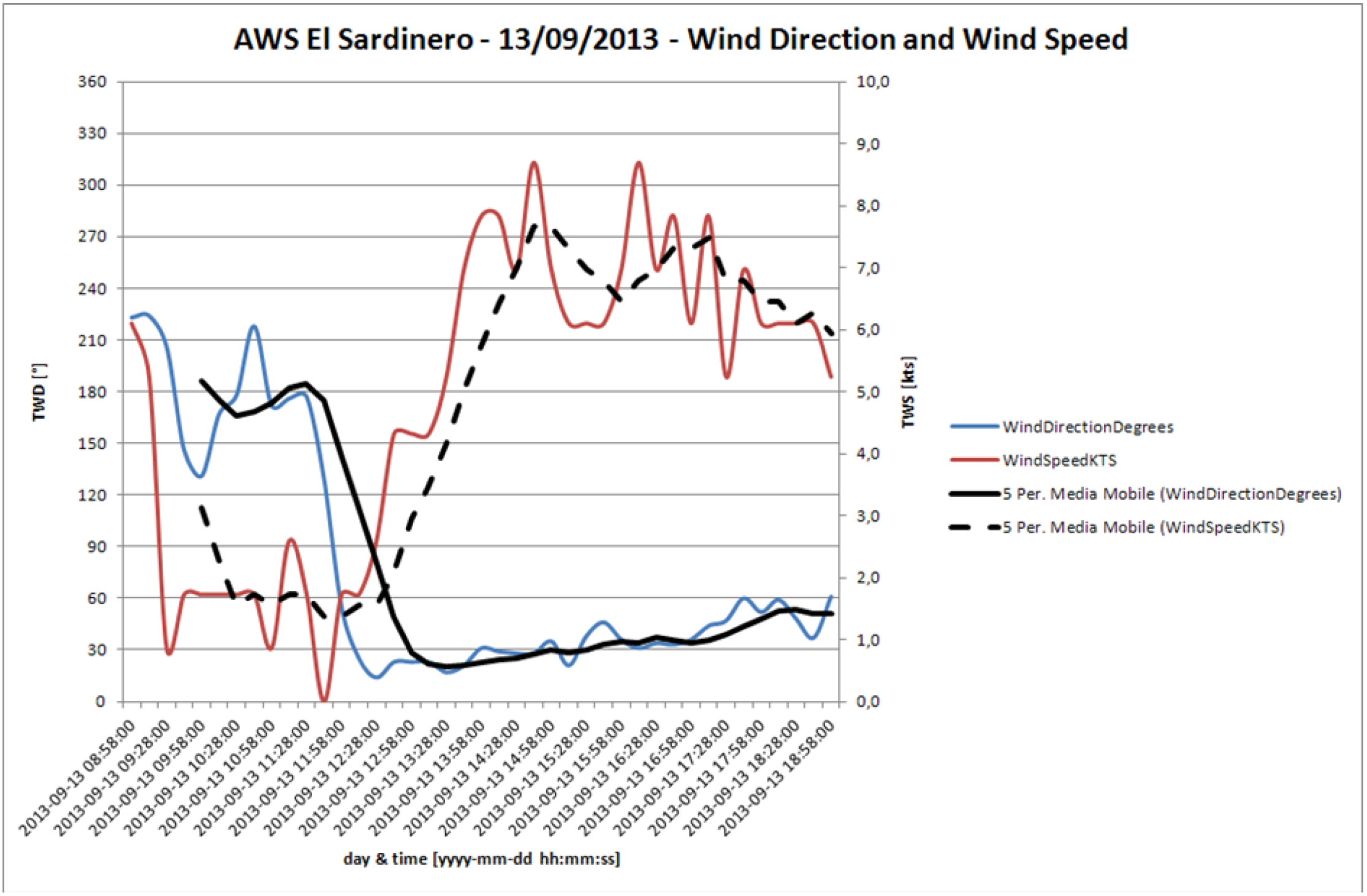
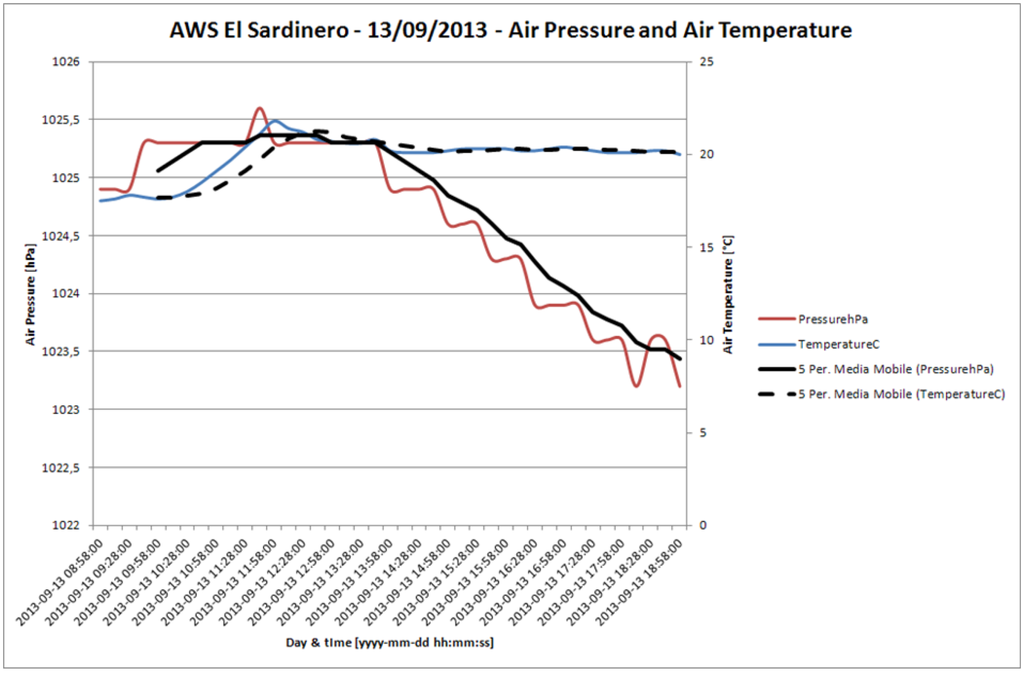
Figure 31. Air temperature (blue line) and atmospheric pressure (red line) measured by the ICANTABR27 station on September 13, 2013. The moving average (factor 5) for air temperature (black dashed line) and for wind speed (black solid line) are also shown.

Figure 31. Air temperature (blue line) and atmospheric pressure (red line) measured by the ICANTABR27 station on September 13, 2013. The moving average (factor 5) for air temperature (black dashed line) and for wind speed (black solid line) are also shown.

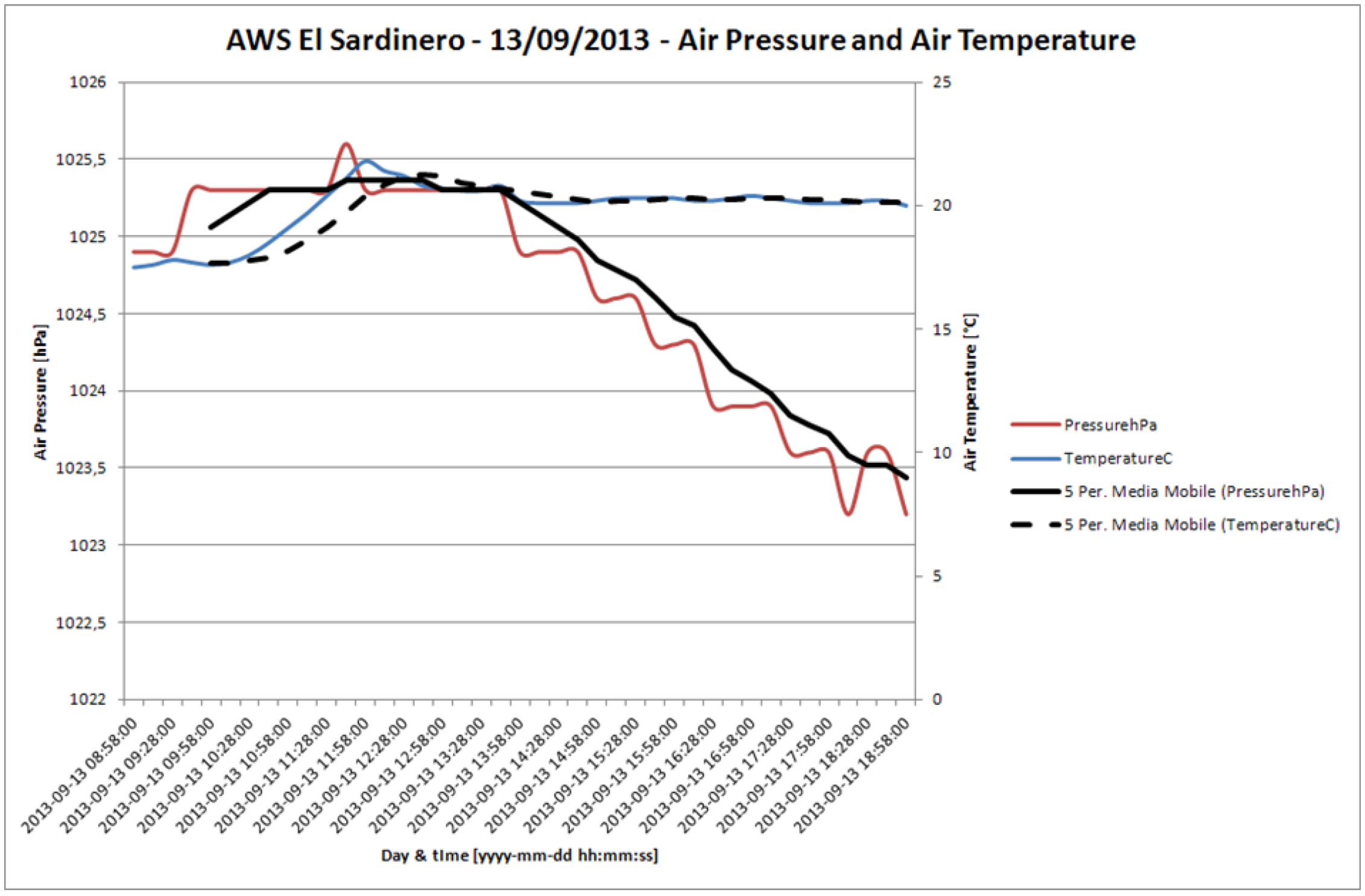
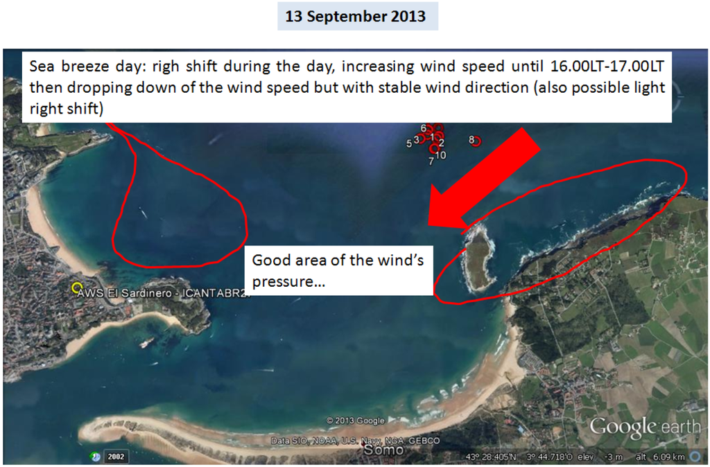
Figure 32. “Call book” for the situation characterized by sea breeze and null or weak gradient wind from SW over the race course.

Figure 32. “Call book” for the situation characterized by sea breeze and null or weak gradient wind from SW over the race course.

4. Conclusions

The results obtained in this study have shown high reliability and confirm that the proposed methodology opens the door to a new “future” in the analysis of sports performance in sailing.

The new technologies of computer analysis are well matched with the more classical sports analysis techniques. Without distorting the instinct which is characteristic of champions and allows them to freely express themselves according to their “feeling”, it is possible, however, to improve their performance by analyzing with new methodologies (such as the one presented in this research) the race courses and the associated strategy.

These new methodologies must be handled by a specialized technician (“Weather Coach”) that must constantly deal with the sailing coach. The latter will then filter out the information to the athletes avoiding overloading them with data and images but helping them to get a simplified "picture" of the regatta field that they can use during the race.

It is useful to suggest to coaches to organize “training” sessions at ground where also athletes must be invited. From this learning phase, the athletes will gain the most useful information to develop their strategy.

References

- Thornes, J.E. The effect of weather on sport. Weather 1977, 32, 258–268. [Google Scholar] [CrossRef]
- Spellman, G. Marathon running an all-weather sport? Weather 1996, 51, 118–125. [Google Scholar] [CrossRef]
- Pezzoli, A.; Moncalero, M.; Boscolo, A.; Cristofori, E.; Giacometto, F.; Gastaldi, S.; Vercelli, G. The meteo-hydrological analysis and the sport performance: which are the connections? The case of the XXI Winter Olympic Games, Vancouver 2010. J. Sports Med. Phys. Fit. 2010, 50, 19–20. [Google Scholar]
- Fleming, P.; Colin, Y.; Dixon, S.; Carré, M. Athlete and coach perception of technology needs for evaluation running performance. Sports Eng. 2010, 13, 1–18. [Google Scholar] [CrossRef]
- Lobozewicz, T. Meteorology in Sport; Sportverlag: Frankfurt, Germany, 1981. [Google Scholar]
- Kay, J.; Vamplew, W. Weather Beaten: Sport in the British Climate; Mainstream Publishing: London, UK, 2002. [Google Scholar]
- Pezzoli, A.; Cristofori, E. Analisi, previsioni e misure meteorologiche applicate agli sport equestri. In Proceedings of the 10th Congress New Findings in Equine Practices, Druento, Italy, 31 October 2008; Centro Internazionale del Cavallo: Druento, Italy, 2008; pp. 38–43. [Google Scholar]
- Olds, T.S.; Norton, K.I.; Lowe, E.L.; Olive, S.; Reay, F.; Ly, S. Modeling road-cycling performance. J. Appl. Physiol. 1995, 78, 1596–1611. [Google Scholar] [PubMed]
- Peiffer, J.J.; Abbiss, C.R. Influence of environmental temperature on 40 km cycling time-trial performance. Int. J. Sports Physiol. Perform. 2011, 6, 208–220. [Google Scholar] [PubMed]
- Pezzoli, A.; Baldacci, A.; Cama, A.; Faina, M.; Dalla Vedova, D.; Besi, M.; Vercelli, G.; Boscolo, A.; Moncalero, M.; Cristofori, E.; et al. Wind-wave interactions in enclosed basins: The impact on the sport of rowing. In Sport Physics; Clanet, C., Ed.; Ecole Polytechnique de Paris: Paris, France, 2013; pp. 139–151. [Google Scholar]
- Pezzoli, A.; Cristofori, E.; Moncalero, M.; Giacometto, F.; Boscolo, A. Effect of the environment on the sport performance. In Proceeding of the International Congress on Sports Science Research and Technology Support, Vilamoura, Portugal, 20–22 September 2013; SCITEPRESS: Portugal, 2013; pp. 167–170. [Google Scholar]
- Buchheit, M.; Voss, S.C.; Nybo, L.; Mohr, M.; Racinais, S. Physiological and performance adaptations to an in-season soccer camp in the heat: association with heart rate and heart rate variability. Scand. J. Med. Sci. Sports 2011, 21, e477–e485. [Google Scholar] [CrossRef] [PubMed]
- Opatkiewicz, A.; Williams, T.; Walters, C. The effects of temperature, travel and time off on Major League soccer team performance. In Proceeding of the World Congress of Performance Analysis of Sport IX, Worcester, UK, 25–28 July 2012; University of Worcester: Worcester, UK, 2012. [Google Scholar]
- Brocherie, F.; Girard, O.; Farooq, A.; Millet, G.P. Climatic influence on home advantage in Gulf Region Football. In Proceeding of the International Congress on Sports Science Research and Technology Support, Vilamoura, Portugal, 20–22 September 2013; SCITEPRESS: Portugal, 2013. [Google Scholar]
- Pezzoli, A.; Cristofori, E.; Gozzini, B.; Marchisio, M.; Padoan, J. Analysis of the thermal comfort in cycling athletes. Procedia Eng. 2012, 34, 433–438. [Google Scholar] [CrossRef]
- Vihma, T. Effects of weather on the performance of marathon runners. Int. J. Biometeorol. 2010, 54, 297–306. [Google Scholar] [CrossRef] [PubMed]
- El Helou, N.; Tafflet, M.; Berthelot, G.; Tolaini, J.; Marc, A.; Guillame, M.; Hausswirth, C.; Toussaint, J.F. Impact of environmental parameters on marathon running performance. PLoS One 2012, 7, e37407. [Google Scholar] [CrossRef] [PubMed]
- Gonzales, B.R.; Hagin, V.; Guillot, R.; Placet, V.; Groslambert, A. Effect of polyester jerseys on psycho-physiological responses during exercise in a hot and moist environment. J. Strengh Cond. Res. 2011, 12, 3432–3438. [Google Scholar] [CrossRef]
- Davis, J.K.; Bishop, P.A. Impact of clothing on exercise in the heat. Sports Med. 2013, 695–706. [Google Scholar] [CrossRef]
- Colonna, M.; Moncalero, M.; Nicotra, M.; Pezzoli, A.; Fabbri, E.; Bortolan, L.; Pellegrini, B.; Schena, F. Thermal behaviour of ski-boot liners: effect of materials on thermal comfort in real and simulated skiing conditions. Procedia Eng. 2014, 72, 386–391. [Google Scholar] [CrossRef]
- Houghton, D. Wind for sailors. Weather 1993, 48, 414–419. [Google Scholar] [CrossRef]
- Del Prete, R.; Pezzoli, A.; Pezzoli, G. Current methods for meteorological and marine forecasting for the assistance of navigation and shipping operation. J. Navig. 1999, 1, 104–118. [Google Scholar] [CrossRef]
- Pezzoli, A.; Franza, M. Safety of navigation, ballast water and meteomarine forecast: Analysis and reliability. J. Navig. 2000, 3, 541–550. [Google Scholar] [CrossRef]
- Pezzoli, A.; Cristofori, E.; Vercelli, G.; Gambarino, C. La comunicazione nello sport della vela: Area di conoscenza, processo o prodotto di progetto? Il caso studio di un Weather Team in un Challenger di Coppa America. Il Giornale Italiano di Psicologia dello Sport 2011, 10, 20–27. [Google Scholar]
- Bethwaite, F. High Performance Sailing, Faster Racing Techniques, 2nd ed.; Adlard Coles Nautical: London, UK, 2011. [Google Scholar]
- Pezzoli, A. A dynamic approach to hydrology problems: a study of disastrous pluviometric events through weather type analysis. Atti. dell’Accademia delle Scienze di Torino 1995, 129, 47–59. [Google Scholar]
- Enke, W.; Spekat, A. Downscaling climate model outputs into local and regional weather elements by classification and regression. Clim. Res. 1997, 8, 195–207. [Google Scholar] [CrossRef]
- Enke, W.; Deutschlander, T.; Schneider, F.; Kuchler, W. Results of five regional climate studies applying a weather pattern based downscaling method to ECHAM4 climate simulation. Meteorol. Z. 2005, 14, 247–257. [Google Scholar] [CrossRef]
- Scire, J.S.; Robe, F.R.; Fernau, M.E.; Yamartino, R.J. A User’s Guide for the CALMET Meteorological Model, 5th ed.; Earth Tech. Inc.: Concord, MA, USA, 2000. [Google Scholar]
- Scire, J.S.; Strimaitis, D.G.; Yamartino, R.J. A User’s Guide for the CALPUFF Dispersion Model, 5th ed.; Earth Tech. Inc.: Concord, MA, USA, 2000. [Google Scholar]
- Enviroware. Available online: http://www.enviroware.com/portfolio/windrose-pro3/ (accessed on 18 February 2014).
- JDC Instruments. Available online: http://www.jdc.ch/en/scientific-line/geos/ (accessed on 6 June 2014).
- Garmin. Available online: http://sites.garmin.com/forerunner910xt/?lang=en&country=US (accessed on 6 June 2014).
- Mosca, S.A.; Graziani, G.; Klug, W.; Bellasio, R.; Bianconi, R. A statistical methodology for the evaluation of long-range dispersion models: An application to the ETEX exercise. Atmos. Environ. 1998, 24, 4307–4324. [Google Scholar] [CrossRef]
- Pezzoli, A.; Tedeschi, G.; Resch, F. Numerical simulation of strong wind situations near the French Mediterranean Coast: Comparison with FETCH data. J. Appl. Meteorol. 2004, 43, 997–1015. [Google Scholar] [CrossRef]
- Wilks, D.S. Statistical Methods in the Atmospheric Sciences; Academic Press: San Diego, CA, USA, 1995. [Google Scholar]
- Houghton, D.; Campbell, F. Wind Strategy, 3rd ed.; John Wiley & Sons Inc.: London, UK, 2006. [Google Scholar]
- Pezzoli, A. Observation and analysis of Etesian wind storms in the Saroniko Gulf. Adv. Geosci. 2005, 2, 187–194. [Google Scholar] [CrossRef]
- Cohen, J. Statistical Power Analysis for the Behavioral Sciences, 2nd ed.; Lawrence Erlbaum: Hillsdale, NJ, USA, 1988. [Google Scholar]
- Rosenthal, J.A. Qualitative descriptors of strength of association and effect size. J. Soc. Serv. Res. 1996, 21, 37–59. [Google Scholar] [CrossRef]
© 2014 by the authors; licensee MDPI, Basel, Switzerland. This article is an open access article distributed under the terms and conditions of the Creative Commons Attribution license (http://creativecommons.org/licenses/by/4.0/).