Abstract
This article presents a Lyapunov precise integral-based analysis method for seismic structures with added viscous fluid dampers. This study uses the full stress algorithm as the optimization method, considering the mean square of interstory drifts as the optimization objective, the position of the damper as the optimization object, and the random vibration analysis method as the calculation method to optimize seismic frame structures with viscous dampers. A precise integral solution is derived for the Lyapunov equation based on the general expression of the Lyapunov differential equation for the damping system under the excitation of a nonstationary stochastic process using two types of modulation functions: and . Finally, the optimal damping arrangement is achieved using this method with a six-layer non-eccentric planar frame. In addition, the optimization results of this study are verified with those in the literature using time-history analysis, which verifies the feasibility and effectiveness of the proposed method. This study provides a method for the optimal configuration of dampers for seismic response of structures, which is beneficial for engineering applications and the protection of seismic structures.
1. Introduction
Since the 20th century, energy dissipation and seismic reduction technologies have played an important role in passive seismic reduction control. In recent years, earthquake disasters have become frequent, and traditional seismic technology can hardly satisfy people’s requirements for structural safety and comfort. In this context, damping and isolation technologies have become the primary option for many important buildings to reduce seismic damage. Many studies have been conducted in the field of seismic design, particularly in the placement of dampers. These have focused on determining an efficient and effective method of damper arrangement based on numerous methods for optimizing damper schemes proposed in previous studies.
Energy dissipation technology is commonly used to reduce earthquake damage to building structures [1]. When energy dissipation design is optimized, a better dissipation effect can be achieved by installing a few energy dissipaters at key positions in structures [2,3,4,5,6,7]. The optimization of viscous fluid dampers in the design of energy dissipation is based on the interstory drifts, story shear, and transfer function of the response as the optimization targets; and the structural member dimensions, number of viscous fluid dampers, parameters, and positions as the optimization objects. Subsequently, optimization is performed using control algorithms, such as sequential search analysis (SSA), the gradient method, and the genetic algorithm.
Zhang [1] proposed the use of SSA to optimize the location and number of viscoelastic dampers. SSA takes the mean square value of the structural interstory displacement obtained from the solution of random vibration theory as the optimization target, analyzes the original structure without additional dampers to calculate the mean square value of interstory displacement, arranges the first damper on the floor with the largest mean square value of interstory displacement, modifies the structural stiffness matrix and damping matrix after the additional dampers, and then completes the arrangement of all dampers sequentially through iteration. This method was explored in subsequent studies [2,3,4,5,6,7]. However, SSA probes potential positions for the dampers of a structure; therefore, the search time is proportional to the minimum number of dampers, and the number of dampers required to achieve the best damping effect is affected by the range of the dampers. Therefore, for the optimal placement of a damper in a three-dimensional structure, the search time increases rapidly with the number of layers and frames of the structure, and it easily falls into the dilemma of local optimal solutions.
In addition to SSA, genetic algorithms are often used for damper optimization. Genetic algorithms are employed to encode each possible solution of a problem as a separate individual, i.e., the “chromosome” of the genetic problem. The first step of the computation requires that we evaluate the randomly generated individuals—the initial solution—against the selected optimization objective and obtain a fitness value from the evaluation. The second step is to use this fitness value as the basis for selecting a chromosome that can be used to create the next generation by following the law of superiority and inferiority. Finally, the chromosomes selected in the second step are randomly combined using crossover and variation operators to obtain new individuals having a better performance than the previous generation [8]. Furuya [9] proposed the optimization of damper parameters, type, and damper position using a genetic algorithm by determining the objective function as a weighted value of the pair of the maximum interstory displacement and acceleration. The interstory displacement and acceleration were obtained by analyzing the structure using finite element software. In the same year, Xu proposed a mathematical model that can optimize the parameters of frictional energy dissipation bracing under seismic excitation using genetic algorithms to achieve the desired seismic reduction with minimal energy dissipation bracing stiffness [10]. Zhou simplified the mean square value of the interlayer displacement by introducing a real code genetic algorithm with a robust critical excitation method to minimize the total additional damping by optimizing the damper distribution [11]. Although the genetic algorithm can achieve the global optimal control effect, its optimization process is more complicated and the computation time is longer.
Whether SSA, the genetic algorithm, or the full stress algorithm in this study is used, the structural response must still be computed and analyzed. Therefore, in addition to the iterative process, most optimization calculations are performed using time-history and response-spectrum analyses. The time-history method has a relatively simple calculation process, but it is computationally intensive and extremely dependent on the selected span of time histories. Studies have shown that the responses obtained from the time-history analysis of several seismic curves recorded at several stations that are not far apart under the same earthquake may differ several times [12,13]; furthermore, it is not a good option for optimizing the viscous damper scheme to use a fixed seismic wave for the response calculation. Although the response-spectrum method is an approximate method based on random vibration theory [14], it cannot fully consider the probabilistic statistical properties of earthquake occurrence. Therefore, this study uses a modulated stochastic process as the excitation load.
Several researchers have created optimal seismic designs of passive vibration control devices by applying the random vibration theory. The virtual excitation method for the problem of random vibration was first proposed by Lin, who transformed the analysis of random vibrations into a deterministic dynamics problem of the structure by assuming virtual excitation [15]. Subsequently, Lin extensively studied the random response problem under the excitation of a nonsmooth random process. Because the virtual excitation method requires solving the response power spectrum of the structure at a series of discrete frequency points, the response power spectrum density of the structure is integrated over the entire frequency domain to obtain the variance of the response [16]. This process requires numerous dynamic response calculations, and only approximate solutions can be obtained. To address this, Zhong proposed a fine-integration algorithm that can efficiently and accurately calculate the dynamic response of a linear structure under a specific load excitation [17,18]. Accordingly, numerous studies have been conducted. Wu and Li deduced equations of motion for single-story eccentric structures with different forms of eccentricity under different viscous damper distribution schemes. They solved the variance matrix of the response using the Lyapunov equation in the random vibration and optimal control theories, built the target function according to the variances of translation and torsional displacement in the matrix, solved the minimum value to determine the optimal eccentric position of viscous dampers, and numerically calculated typical examples using this theory to verify the importance of the method to aseismic design [19]. Gomez used Lyapunov differential equations for the optimal design of nonlinear energy sink devices in structures under nonsmooth stochastic excitation [20]. Xu studied a multiobjective optimization problem for nonlinear structures subject to stochastic dynamic excitation [21,22,23]. In other scenarios, more advanced methodologies [24] have been adopted.
In this paper, a new optimization scheme is proposed for arranging dampers in a vibration-damping structure using viscous dampers. The scheme is based on the equations of motion, considering the nonsmooth stochastic excitation process, and achieves a full stress design with the mean square value of interstory displacement as the optimization objective through iteration. In this process, the state-space equation of the damping structure was first established based on the equation of motion, in which the damping matrix considered the effect of additional damping of the damper, and the excitation load was the random vibration load reduced from the state equation to the Lyapunov differential equation with an unknown quantity as the mean square value of the interstory displacement. Finally, the equation was solved using the fine-integration method to obtain the mean square value of the interstory displacement. With the determined total additional damping case, the initial case was iterated using the full stress algorithm, such that the mean square value of the displacement between the layers was smoothed, and the damping distribution at this time was very effective in controlling the story drift of the added damping structure. Finally, taking the six-layer shear frame used by Takewaki [25] as a numerical example, the damping optimization results were first obtained by redistributing the damping using the method proposed in this study with the modulated Kanai–Tajimi spectrum as the excitation. The optimization results of this study were validated using time-history analysis.
2. Lyapunov Equation of White Noise for Dissipation Structures
2.1. State-Space Expression for the Equations of Motion of the Damping Structure
In earthquake engineering applications, the equation of motion for linear multiple-degree-of-freedom (MDOF) structures with viscous fluid dampers is set as follows [26]:
where x is the displacement component in global coordinates, M is the mass matrix, C is the damping matrix, Cd is the additional damping vector, K is the elastic stiffness matrix of the structures, e is the excitation matrix with an input of 0 or 1, ag(t) is the ground motion acceleration vector, and the dot on top represents the derivative with respect to time.
The optimization of viscous dampers involves optimizing the additional damping vector Cd The optimized arrangement of dampers exists in two cases: planar and vertical optimized arrangements, and the optimization process requires the use of the floor response of the structure. Therefore, a conversion relationship should be established between the structural floor response and the response of each damper. Equation (2) can then be used to convert the damping of individual dampers to additional damping in global coordinates.
Because the additional dampers may be arranged anywhere in the plane or three-dimensional frame, a transformation matrix is required to represent the additional damping in global coordinates:
In Equation (2), denotes the equivalent linear damping of each damper, nd is the total number of dampers, and T is the transformation matrix that converts the displacement from the original global coordinates to the local coordinates of the additional dampers; T includes both planar and vertical transformations.
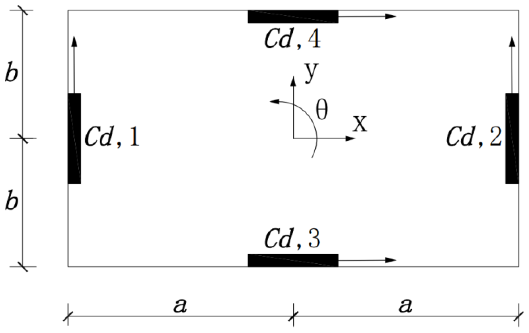
For the structural plane shown in Figure 1, let x and y be the global coordinates of the plane, and let be the damper number. To achieve the interconversion between the overall displacement of the plane and the displacement of each damper, we use the plane conversion matrix (Equation (3)).
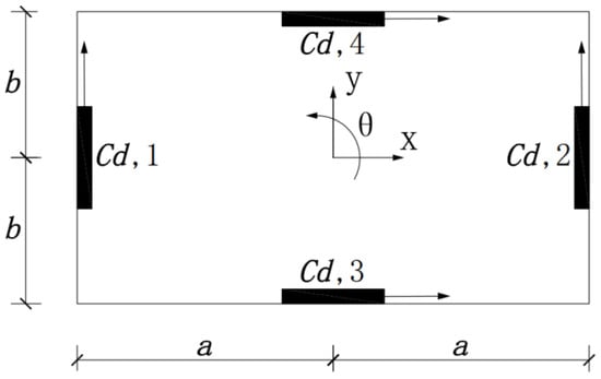
Figure 1.
Structural plane with dampers.
The rows in the matrix represent the positions of the dampers numbered , and the columns represent the displacements in the x, y, and directions, and three DOFs in the damper arrangement. For example, if a unit displacement is applied in the x-direction, the dampers numbered and will not produce a displacement, and the dampers numbered and will produce a unit displacement. Thus, the first column of the transformation matrix is . The second and third columns of the transformation matrix are and , respectively.
For the vertical arrangement of the dampers, the conversion of the overall structural displacement to the horizontal displacement under individual dampers can be represented by the vertical conversion matrix Tp.
Column i in matrix is the unit displacement applied at layer i of the structure, resulting in the displacement of the dampers in each layer.
The conversion matrix T of the multistory structure must consider both the planar and vertical conversion matrices. First, the overall displacement of the structural plane must be converted into the displacement of the in-plane dampers by the plane conversion matrix , followed by the conversion of the displacement of the structure to the horizontal displacement of the individual dampers by the vertical conversion matrix . Therefore, the elements in the plane conversion matrix are multiplied by the vertical conversion matrix to obtain the chunking matrix , which constitutes the conversion matrix T of the multilayer structure.
Therefore, the displacement of the local coordinates at the damper position can be calculated using Equation (5) [26].
Equation (1) is a second-order differential equation that describes the equations of motion in terms of a system of first-order differential equations composed of state variables by introducing the concepts of state vectors and spaces.
The state of the structure at any time can be represented by the velocity and displacement at that time. Thus, the state variable is introduced, and Equation (1) is expressed in the form of Equation (6):
where , and the matrixes A, H, and D are calculated using
2.2. Lyapunov’s Equation in White Noise
Currently, the methods for solving the dynamic response of structures under random vibrations include time-domain analysis and frequency-domain analysis, in which the correlation function of the excitation is integrated in the time domain or the spectral density function of the excitation is integrated in the frequency domain to obtain the correlation function of the response. The time difference of the random process is , and is the variance of the response under the smooth process. The Lyapunov equation can be used to solve the variance of the response of the vibration system easily and quickly, without integrating the correlation function or power spectral density. Compared with deterministic seismic response analysis, the advantage of using the Lyapunov equation for seismic response analysis of seismic control structures is that the seismic excitation is a stochastic process, and the optimization scheme is not affected by individual seismic waves.
For the ideal white noise excitation, because its mean square value is infinite (Figure 2), which is physically impossible, and its probability density function can hardly be discussed, the white noise can be considered as the limiting case of colored noise. While Y(t) is assumed to be the stationary colored noise, its correlation function and power spectral density are defined in Equation (8):

Figure 2.
Colored and white noises.
As shown in Figure 2, during , the colored noise Y(t) becomes the ideal white noise, which is represented by W(t). The correlation function and power spectral density (9) of W(t) are obtained by calculating the limits using Equation (8):
If the excitation acting on the MDOF system is the white noise vector W(t), its mean value is zero, and the variance matrix is represented by Equation (10).
where S0 is the power spectrum matrix of the excitation; the diagonal elements si,j in the matrix are the self-power spectral densities of each white noise; and the nondiagonal elements are the mutual power spectral densities.
The state-space equations structured according to Equations (6) and (10) can be expressed in the form of Equation (11) with the same variable A as in Equation (7) and the variable .
Solving Equation (11), and when is zero, the general solution of the chi-square differential equation in Equation (11) takes the form of Equation (12).
Subsequently, the full solution of Equation (11) when H is not zero is
in Equation (12) is the initial condition at . Often, the initial condition is independent of the excitation; therefore, the average value of the response can be obtained based on Equation (13) as in Equation (14):
The correlation function matrix of the response is calculated using Equation (15).
where is the smooth white noise, its intensity function is D, and its autocorrelation function is calculated using Equation (16).
Subsequently, Equation (15) becomes
In Equation (17), by making t1 = t2 = t, the variance matrix of the response can be obtained using
Taking the derivative with respect to t, it becomes
Because , the Lyapunov differential equation satisfied by the variance matrix Q is
Equation (20) is called the Lyapunov equation. It reflects the nature of the variance EZ(t) of the response Z. When the input excitation is white noise and the structural response is smooth, the variance is not affected by time. Therefore, the equation can be solved under white noise excitation. In this study, we primarily consider the computational analysis under nonsmooth excitation and use the fine-integration method to solve it based on Equation (20) for further derivation.
3. Stochastic Optimization Analysis of Dissipation Structures
3.1. Optimization Method for Dissipation Structures Based on Random Response
The actual ground motion is a nonstationary process. The stationary random process excitation can be preliminarily analyzed for ground motions with long durations of strong components.
In 1993, Inaudi first designed a passive vibration control of plane frame structures using the Lyapunov equation [27]. During the design process, a friction damper was used to optimize the damper, with the maximum mean square value of the interstory displacement as the goal. Because the Lyapunov equation adopts white noise excitation, the bandwidth of the actual ground motion input affected the optimization of dampers. For the same total additional damping, the positions at which dampers are optimized under narrowband and broadband excitations are different [28]. Thus, it is not appropriate to take the white noise process as the approximate value of ground motion, but this scenario will not occur in the optimization design based on the Lyapunov equation and time history. However, in some cases, filtered white noise can also be used as an input for structures. At this point, matrices A, H, and D in Equation (7) must be further modified.
The steady-state response variance of the controlled interstory displacement can be obtained using the following equation [26]:
The elements on the diagonal of matrix P in Equation (21) are the mean square values of the interstory displacement. In Equation (21), is obtained by solving differential Equation (20).
When the distribution of dampers is appropriate, the total damping required to satisfy the damping requirements is smaller. Therefore, this section aims to determine the best damping distribution scheme under white noise excitation to minimize the total damping required for the structure while ensuring that the mean square value of the interstory displacement of all floors of the frame is not larger than the given allowable value.
3.2. FSD Optimization
The FSD algorithm [29] is widely used to optimize the design of structures under dead loads. FSD means that the stress in the member reaches the allowable stress of the material such that the carrying capacity of the material is fully utilized. Generally, FSD is solved using iterative methods. First, the member whose section area is known is analyzed to obtain the maximum internal force. Second, the new section area of the member is solved according to the design specification and allowable stress. The full stress of the member under the most unfavorable load can be obtained using the above iterative process.
Similarly, to fully understand the role of dampers, we introduce the concept of the full stress of members to the optimization of damping and its distribution to realize the “full stress” of the mean square value of the interstory displacement of structures. During the iterative process, the Lyapunov equation is used to calculate the mean square value of the interstory displacement of the given additional damping structure, and the recursive relation is used to redesign the additional damping of the structure. The above steps are repeated until the full stress of the mean square value of the displacement is reached, as shown in Equations (22) and (23):
where cdi(k) is the ith component of the damping vector in the kth iteration, q is the convergence parameter, pii(k) is the ith component of the performance index (with cd(k) as the damping vector) in the ith iteration (see Equation (2) for the definition), pi,I is the component in the ith column and ith row of the matrix P, and is the prescribed limiting value. cdi(k) and pii(k) are values at the same position, namely the same story. Meanwhile, the selection of the convergence parameter q will affect the calculation efficiency of this method. When the q value is large, this method is more stable and converges more easily, but at a slow rate. For linear problems, the q value can be 0.5; for nonlinear problems, a q value of 5 is more appropriate [30].
3.3. Kanai–Tajimi Spectrum Excitation
The Kanai–Tajimi model, whose frequency is distributed unevenly, can better reflect the frequency characteristics of actual ground motion [31]. The Kanai–Tajimi model assumes that the power spectral density function of a bedrock earthquake is S0, which is ideal white noise with a mean value of zero. The upper soil layer of the bedrock is simplified as a linear single degree of freedom (SDOF), which filters the bedrock white noise. The power spectral density function of this noise model can be represented by Equation (24) [32].
From [33], the relationship between spectral intensity S0 and seismic intensity I can be expressed as in Equation (25).
In Equation (25), S0 is the power spectral density of the bedrock white noise, which reflects the intensity of seismic excitation; and are the characteristic frequency and characteristic damping ratio, respectively, of the site, which are related to the hardness of the site. The suggested values of and are listed in Table 1 [34].

Table 1.
Parameters of the Kanai–Tajimi spectrum.
The Kanai–Tajimi spectrum, which considers that the spectrum characteristics of ground motion are affected by the characteristics of the top soil layer and are close to those of actual ground motion, is currently widely used. The Kanai–Tajimi spectrum reflects the overall changing trend of the power spectral density function of ground motion [32]. When is zero, the power spectral density function approaches the power spectral density of white noise; however, the actual power spectrum should approach zero in this case. Therefore, this model overestimates the low-frequency energy of the ground motion. Thus, the results of the Kanai–Tajimi spectrum analysis of low-frequency structures are unreasonable, and the model is only suitable for random seismic response analysis of structures with middle and high natural frequencies.
The power spectral density function of the Kanai–Tajimi spectrum is essentially a filter process of white noise, in which the bedrock layer covered by it is simplified to a linear SDOF filter. The filtration equation is
In Equation (26), is the absolute acceleration of the ground, is the relative acceleration with respect to the bedrock, and is the acceleration of the bedrock, which is assumed to be a zero-mean white noise process.
3.4. Lyapunov Differential Equation for Dissipation Structures under Nonstationary Excitation
Equation (20) is the Lyapunov equation under white noise excitation. Let , f(t) be the uniform modulation evolving random excitation, and g(t) be the slow-varying uniform modulation function with smooth Gaussian white noise.
Equation (27) is the Lyapunov differential equation that is satisfied by the variance matrix Q of the structural response, and the variance matrix of the response can be obtained by solving this differential equation.
To solve this equation, we first set the constant term of the Lyapunov differential equation to zero, and then the chi-square Lyapunov differential equation can be obtained.
Taking the derivative of both sides with respect to t, is the particular solution of Equation (27). Let ; therefore, when the initial value is not zero, the solution of Equation (27) is
When considering only the scenario in which and when the initial value is not zero, the equation can be solved separately and the superposition principle can be applied. As the initial value is zero,
Because , ; therefore, at ,
Similarly, the equation for the double step at 2t can be expressed as follows:
When deriving the specific equation for time variance, the modulation functions g(t) = 1 and should be considered. Assuming , g(t) = 0, the variance of the response at .
- (1)
- The modulation function is a constant 1.
When g(t) = 1, G(t) and J(t) are constants, assuming J(t) = J0, when , Equation (30) is transformed into
Subsequently, when ,
Similarly, the equation for the double step at 2t is as follows:
- (2)
- The modulation function is time-dependent.
When , , then at , Equation (30) is transformed into
Subsequently, the integration equation for the equal step at is
Subsequently, the corresponding equation for the double step is
The above are calculation equations for the response variance when the modulation functions are one and ; corresponding calculation equations can also be established for other simple modulation functions to solve the variance matrix Q of the structural response.
4. Results and Discussion
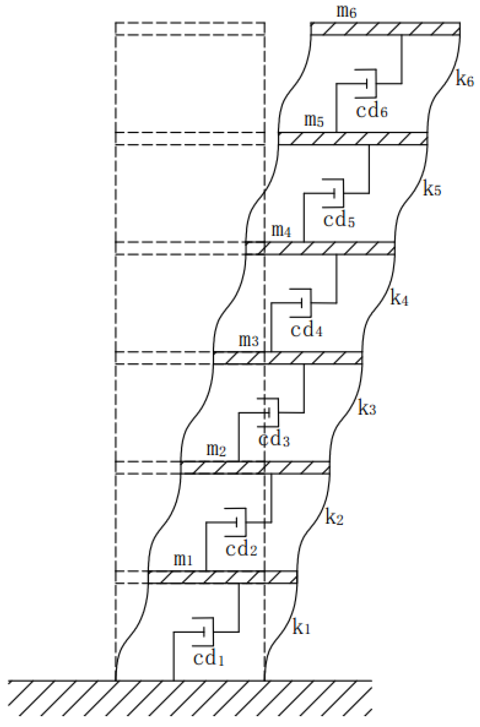
In 1997, Takewaki [25] applied the minimum transfer function to optimize the energy dissipation of a six-story plane shear frame (see Figure 3). All stories of the shear frame had the same mass (m1 = m2 = …m6 = 0.8 × 10⁵ kg); the stiffness was evenly distributed in each story (k1 = k2 = …k6 = 4.0 × 10⁷ N/m); the structure’s damping ratio ξs = 2% for the first six orders. To elaborate on the precise integral solution process of the Lyapunov differential equation and confirm its feasibility, this frame was considered to have filtered white noise suddenly applied on it. The Kanai–Tajimi spectrum and the Lyapunov differential equation satisfied by the structural response variance matrix were precisely integrated to obtain the variance matrix of the response.

Figure 3.
Six-story plane frame.
After treatment using the static condensation method, the mass and stiffness matrices of the structure were expressed as follows:
Using the mass matrix M and stiffness matrix K, we calculated the vibration pattern and frequency of each order of the structure. Given a structural damping ratio ξs = 2%, the Caughey damping coefficient were calculated. Finally, the damping matrix C of the six-story frame was obtained as follows:
If only the lateral horizontal displacement of the frame is considered, the excitation matrix in the equation of motion is , and the displacement transformation matrix is
If the structure is excited using the Sugakinai Kiyoshi model, and the modulation function g(t) = 1 when t ≥ 0, then
where the power spectral density function of is given by Equation (21).
Assuming that the site is a hard-soil site, the characteristic frequency and characteristic damping ratio were set as and , respectively. The peak acceleration of ground motion input in the original example was 0.1 g, and the corresponding seismic intensity in the scale of seismic intensity was degree 7; thus, I = 7 and were obtained using Equation (25). To achieve the accuracy of the calculation, the time step was set to 0.02 s. With a total of 400 steps, the total duration time for the calculation was 8 s.
First, the integration step was equally divided into 2N parts, with N = 20 in general; that is, 220 parts and and .
The initial value of the integral is the at . Because the value of is small, the first few terms of the Taylor expansion ensure sufficient accuracy. The Taylor expansion is calculated as follows:
where is the same as in Equation (7), and In is the 12-order unit matrix. Subsequently, the initial value of is obtained using Equation (33).
Using Equation (35) for the double step and the initial value of the variance matrix , we obtain
After iterating the above equation 20 times, the variance matrix Q of the response at = 0.02 can be obtained. To avoid numerical ill-conditioning, we iterate the above equation 10 times; is replaced by in the last 10 iterations, and the iterative is changed to , thus obtaining the final .
This is the integration process for calculating the variance matrix of the response at . Subsequently, the response variance matrix at 2, 3, … (until 400) was calculated using (34) to obtain the variance matrix of displacement at t = 8 s. For k = 1, 2, 3…399, the following iterative equation was executed:
where the initial value is , and the response variance matrix of the structure is calculated as .
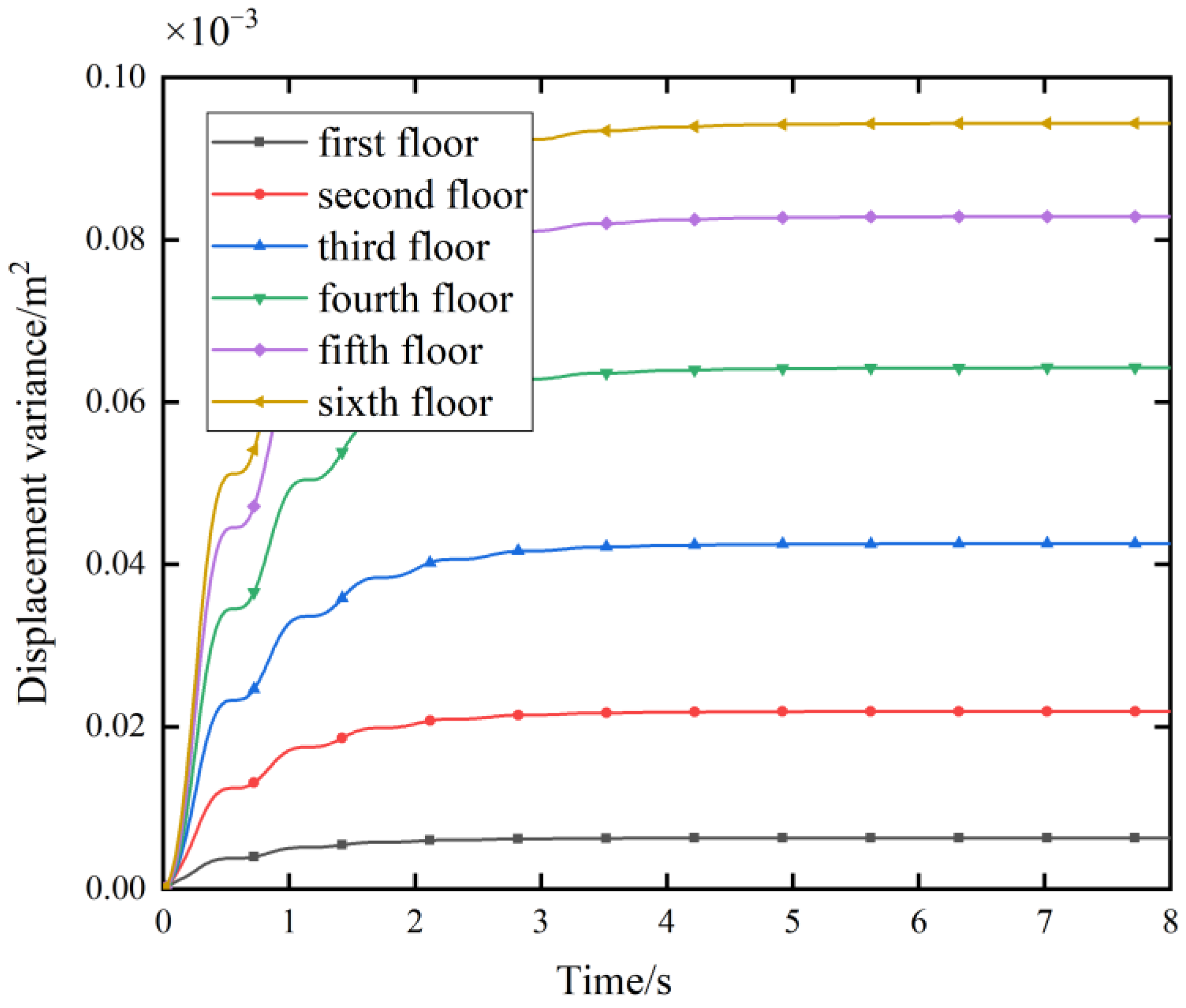
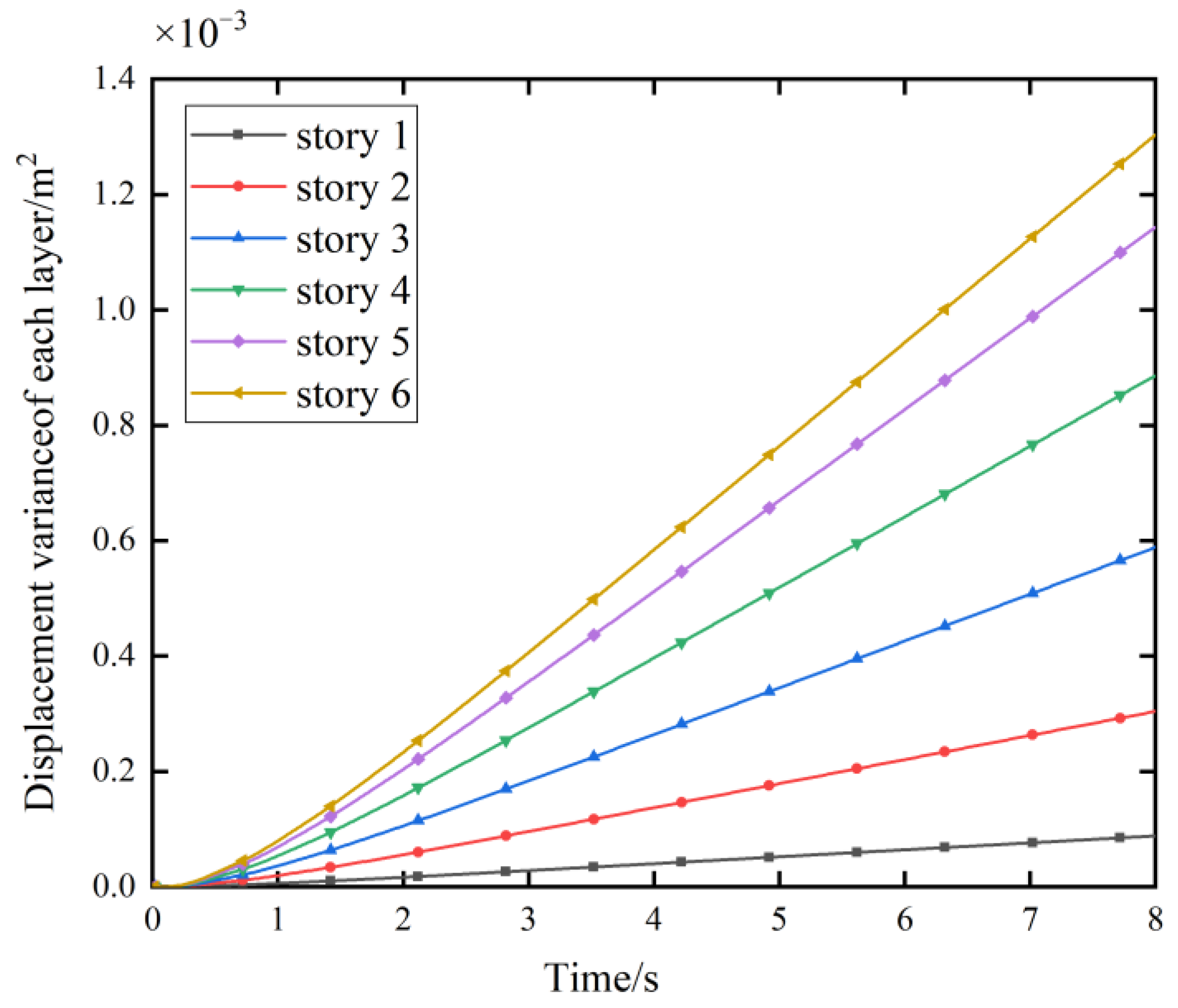
The time-dependent displacement variance curve obtained during the calculation process is shown in Figure 4. The figure shows that the displacement variance of each layer tends to be stationary at t = 8 s. Here, the displacement variance value of each layer is .
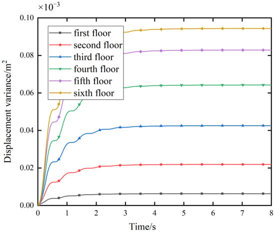
Figure 4.
g(t) = 1: Time-dependent displacement variance.
The displacement variance tends to be stationary at t = 8 s; therefore, the mean square value of the controlled interstory displacement at this time is used as the target function of optimization. The variance matrix is substituted into Equation (21) to calculate the steady-state covariance of the controlled interstory displacement:
where the elements on the diagonal of matrix P are the mean square values of the controlled interstory displacement. The mean square value of the displacement is expressed as follows:
The additional damping matrix in the next iteration derived using Equations (22) and (23) is:
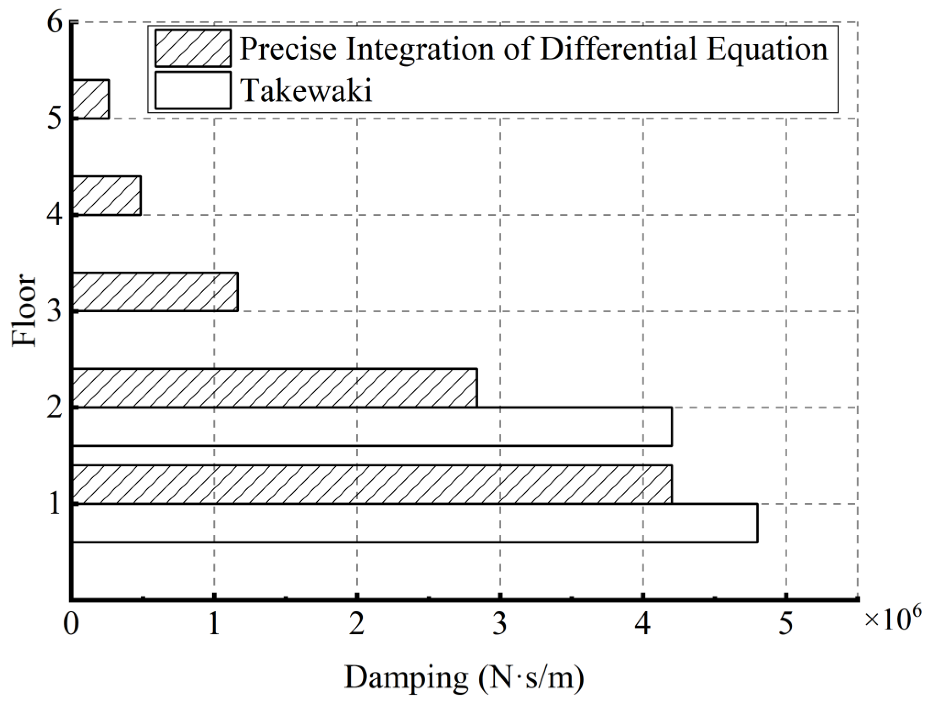
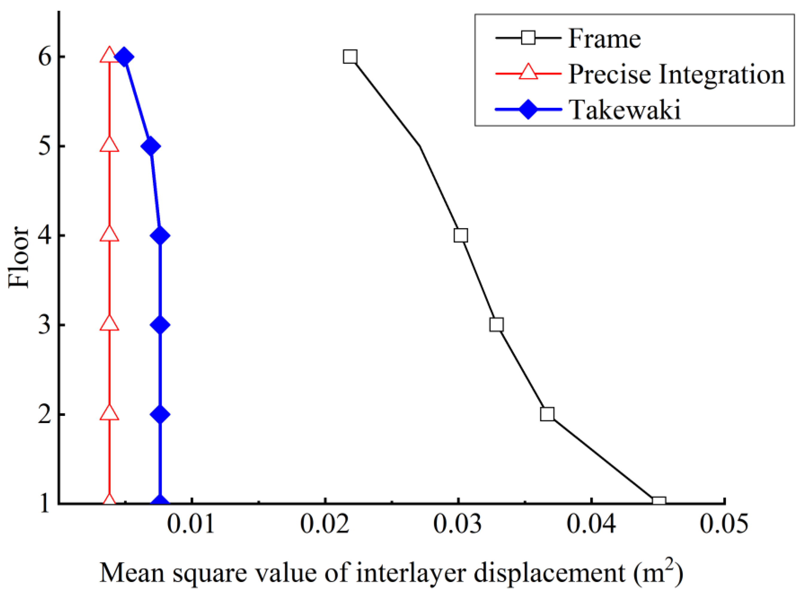
The final optimization results are shown in Figure 5 and Figure 6. Comparing the mean square values of the interstory displacements before and after the additional damping optimization, we observe that before optimization, the mean square values of the displacements of each layer of the structure vary significantly. After optimization, the mean square value of displacement of each layer of the structure is significantly reduced, and the mean square value curve of interstory displacement tends to be uniform. Therefore, the full stress design of the mean square value of interstory displacement of each layer can be achieved when the total additional damping is certain.
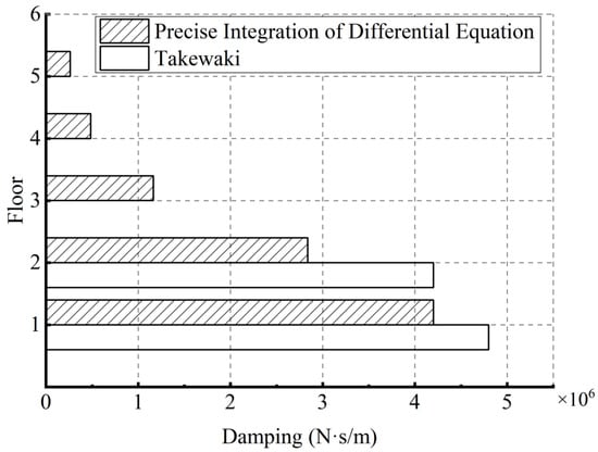
Figure 5.
Six-story shear frame: distribution of damping coefficient by different response calculation methods [25].

Figure 6.
Six-story shear frame: mean squared interstory drifts before and after optimization [25].
After dissipation optimization using precise integration based on the Lyapunov differential equation, the curve of the mean square values of the interstory displacement in Figure 6 is perpendicular to the coordinate axis, which perfectly achieves the fully stressed design of the mean square value of the interstory displacement, and the results are compared with the methods in other studies.
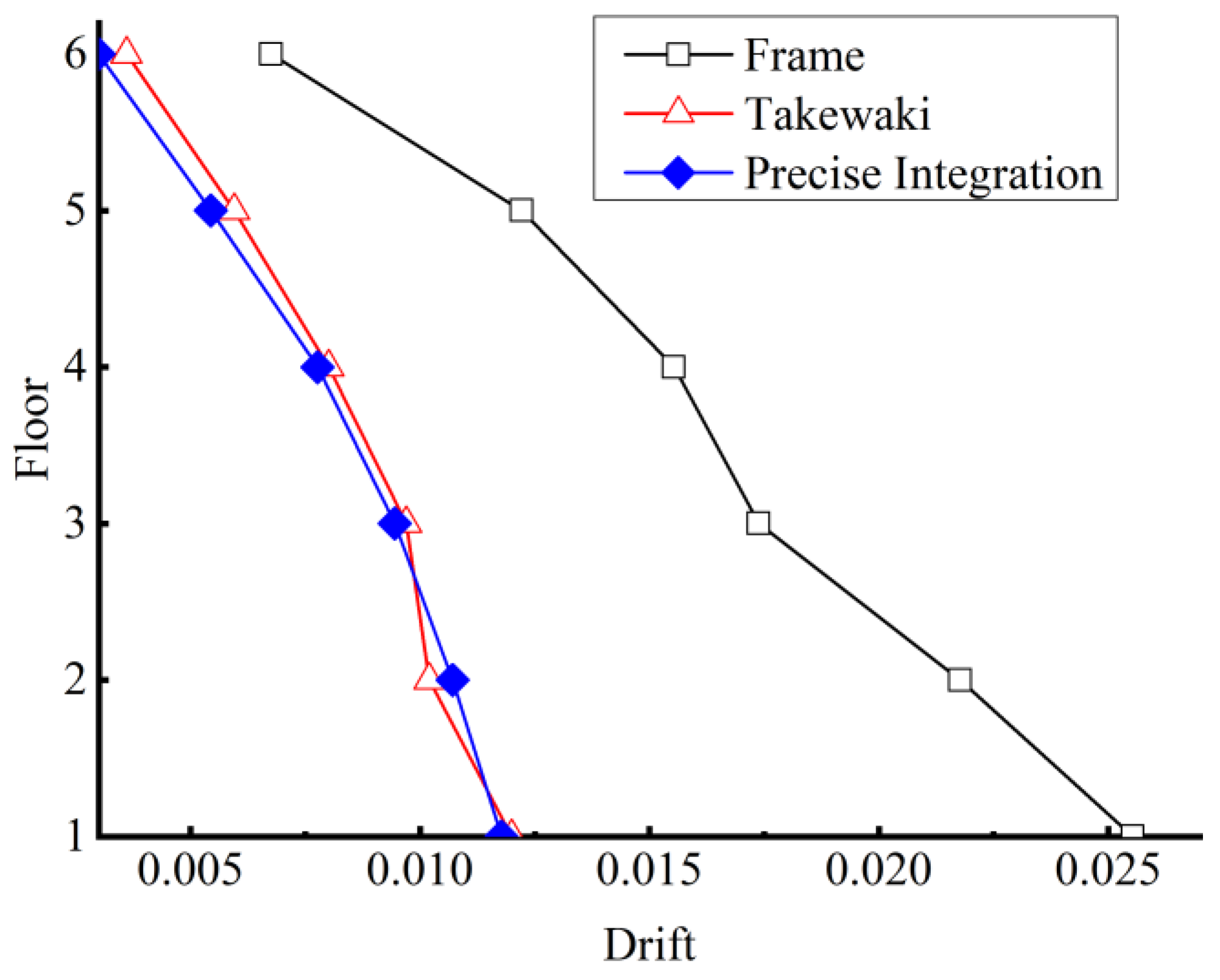
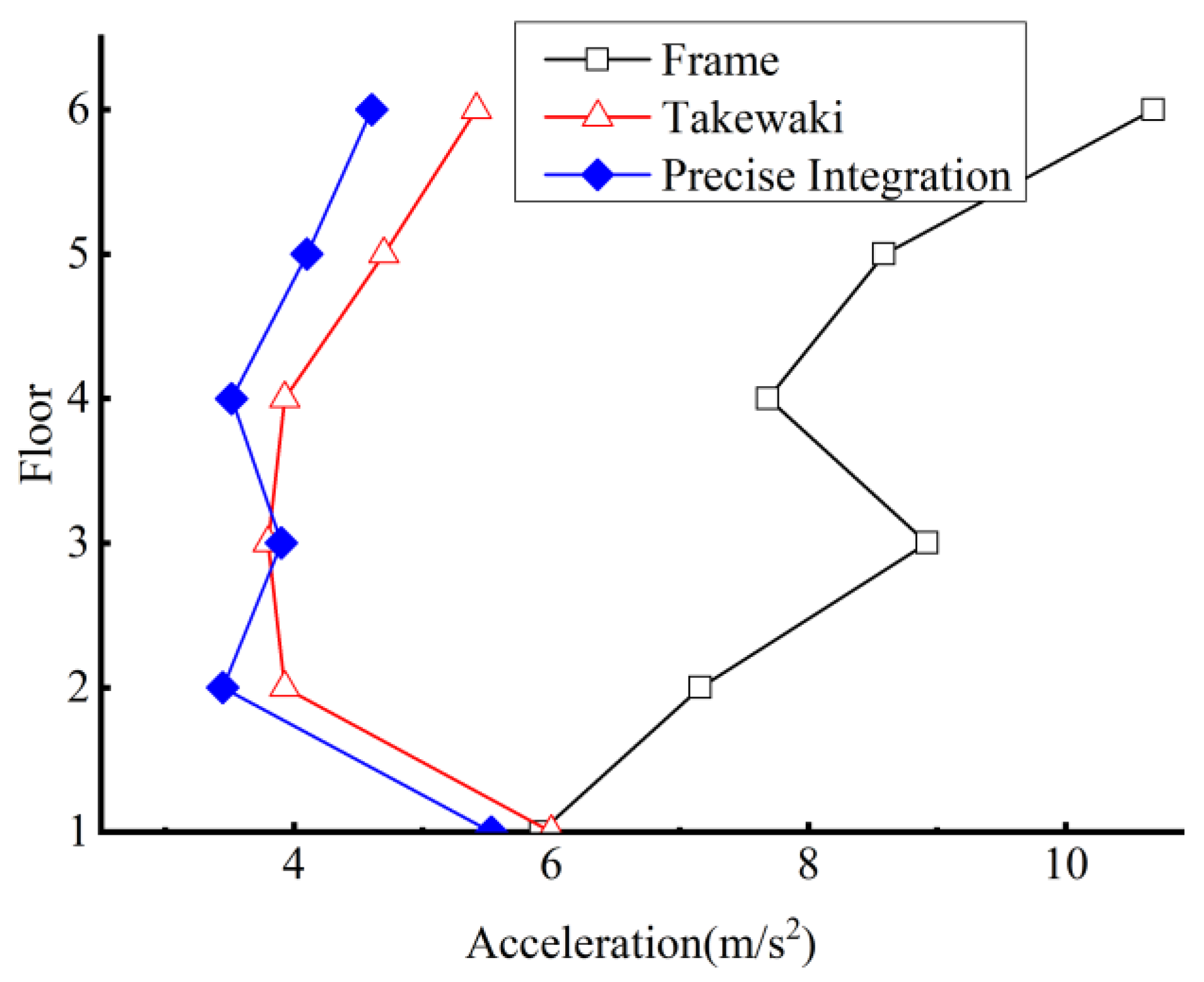
The basic data of the model and optimized additional damping ratio are used to build a finite element model, and the model is subjected to time-history analysis to extract calculated results, such as acceleration and displacement angles. By comparing the obtained interlayer drift ratios (Figure 7) and floor accelerations (Figure 8) of the uncontrolled and damped frame under different response calculation methods, we observe that the optimization based on the Lyapunov differential equation and the optimization based on the method in [25] are the same in structure and excitation. Only the calculation method of the response variance matrix is different, and the optimized interstory drift ratios almost completely overlap, which verifies the correctness and feasibility of the precise integration of differential equations when calculating the response variance matrix.

Figure 7.
Six-story shear frame: Story drifts by different response calculation methods [25].

Figure 8.
Six-story shear frame: Accelerations by different response calculation methods [25].
The above consideration is the optimization of the structure under smooth-colored-noise excitation at g(t) = 1. The model used in the calculation is always in an elastic state, and for elastic models, the effect of considering the descent phase in the modulation function on the calculation results is relatively small. If the modulation function is replaced with , the response variance matrix of the structure under a nonsmooth process can be calculated using the fine integration of the Lyapunov differential equation, and the structure is optimized for damping.
The initial value of the integral is calculated using Equations (39) and (40), and can be obtained using Equation (36).
Subsequently, using Equation (38) for the double step of the modulation function , we obtain
where is the response variance matrix at g(t) = 1. To avoid numerical ill conditioning, we can iterate the above equation 10 times; in the above equation is replaced by in the last 10 iterations, and the iterative is changed to , thus obtaining the final .
The response variance matrix at 2, 3, … (until 400) is calculated using the equal step integration Equation (37) to obtain the variance matrix of displacement at t = 8 s. For k = 1, 2, 3…399, the iterative equation below is executed.
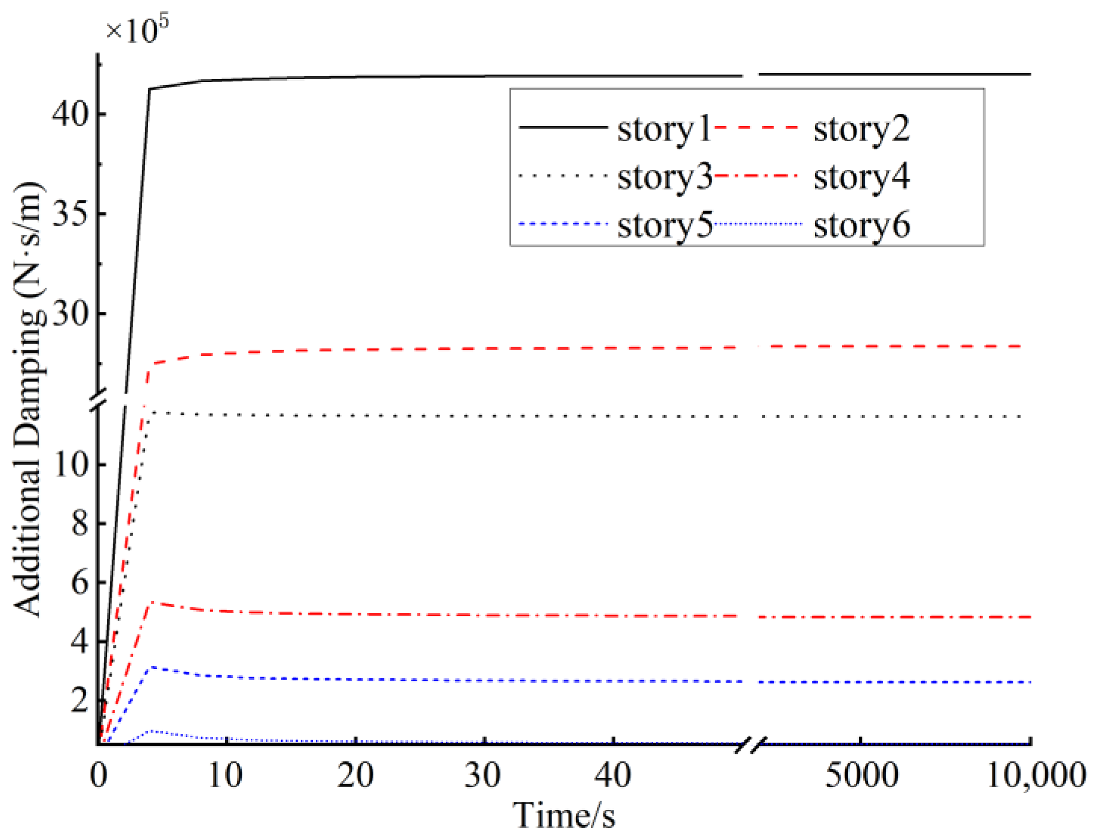
The calculation results are shown in Figure 9. When , the response variance increases rapidly and is strongly nonstationary. Therefore, time t for the response variance matrix affects the final optimization of the damping. The optimization results for different values of t are shown in Table 2.

Figure 9.
: time-dependent displacement variance.

Table 2.
Optimization of additional damping.
The calculation results are shown in Figure 10. Owing to the nonstationary excitations, the optimization results are affected by time. Nevertheless, the distribution of the additional damping changes slightly and tends to be stable over time.
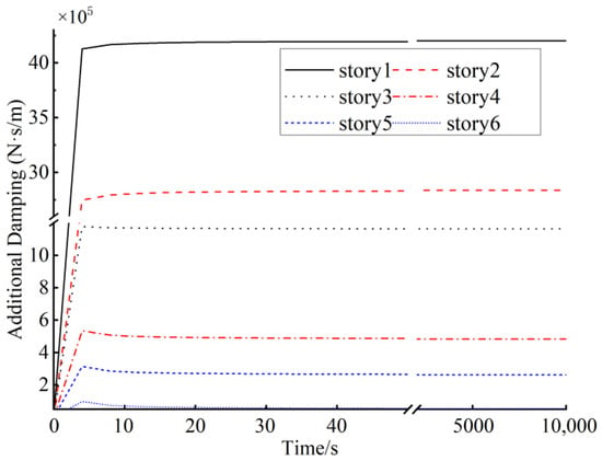
Figure 10.
: optimization of additional damping.
5. Conclusions
In this paper, a structural state-space equation satisfying Lyapunov’s equation under white noise excitation is derived. Subsequently, the equation is combined with the full stress algorithm to derive a damper optimization process for a damping structure under stochastic excitation. Thereafter, the Kanai–Tajimi spectrum excitation is introduced, and the process for the Lyapunov differential equation of the stochastic excitation under the modulation function g(t) = 1 and is derived. Finally, the results of the optimal damping assignment under the two modulation functions are calculated using a numerical example.
(1) The equation of motion for dissipation structures is rewritten as the state equation, and the Lyapunov equation used to solve the random seismic response under white noise excitation is deduced; subsequently, the stochastic optimization of damper positions is achieved using the “full stress” of the mean square value of the displacement as the optimization objective.
(2) Based on the filter equation of the Kanai–Tajimi spectrum, the corresponding Lyapunov equation is established, with its autocorrelation function as the known quantity, achieving the response solution of the dissipation system under colored-noise excitation, the random response solution of dissipation structures under Kanai–Tajimi spectrum excitation, and the stochastic optimization of damper positions.
(3) The extended order vector is introduced to establish the Lyapunov differential equation under evenly modulated random excitation, providing a basis for subsequent optimization design. The precise integration process of the Lyapunov differential equation is deduced, and the Lyapunov differential equation satisfies the random response variance matrix, which is directly solved using precise integration for modulation functions and . Taking a six-story non-eccentric plane frame as an example, the calculated results are compared with those reported in the literature to verify the feasibility and effectiveness of the proposed method.
This study focused on the optimization method of the energy dissipation structure considering random excitation. Nevertheless, the case model in this study is a simple two-dimensional frame that considers only the shear stiffness of the structure and neglects the bending stiffness. Further research on models that consider bending stiffness is required. Furthermore, this study used a relatively simple modulation function, which is only suitable for elastic structures. To obtain optimized results for plastic structures, a more complex modulation function that considers the descent phase should be used for analysis. These are the significant limitations of this model.
Author Contributions
Conceptualization, Y.Z. and W.X.; methodology, W.X.; software, Y.Z.; validation, Y.Z. and W.X.; formal analysis, D.D.; investigation, Y.Z.; resources, D.D.; data curation, W.X.; writing—original draft preparation, Y.Z.; writing—review and editing, W.X. and D.D.; visualization, Y.Z.; supervision, S.W.; project administration, S.W.; funding acquisition, D.D. and W.X. All authors have read and agreed to the published version of the manuscript.
Funding
This research was funded by Six Talent Peaks Project in Jiangsu Province, grant number JY-022; Scientific Research Fund of Multi-Functional Shaking Tables Laboratory of Beijing University of Civil Engineering and Architecture, grant number 2022MFSTL03; Fellowship of China Postdoctoral Science Foundation, grant number 2022M721591.
Conflicts of Interest
The authors declare no conflict of interest.
References
- Zhang, R.H.; Soong, T.T. Seismic Design of Viscoelastic Dampers for Structural Applications. J. Struct. Eng. 1992, 118, 1375–1392. [Google Scholar] [CrossRef]
- Takewaki, I.; Uetani, K. Optimal damper placement for building structures including surface ground amplification. Soil Dyn. Earthq. Eng. 1999, 18, 363–371. [Google Scholar] [CrossRef]
- Takewaki, I. Optimal damper placement for critical excitation. Probabilist. Eng. Mech. 2000, 15, 317–325. [Google Scholar] [CrossRef]
- Sullivan, T.J.; Lago, A. Towards a simplified Direct DBD procedure for the seismic design of moment resisting frames with viscous dampers. Eng. Struct. 2012, 35, 140–148. [Google Scholar] [CrossRef]
- Malekpour, S.; Dashti, F. Application of the Direct Displacement Based Design Methodology for Different Types of RC Structural Systems. Int. J. Concr. Struct. Mater. 2013, 7, 135–153. [Google Scholar] [CrossRef]
- Bahmani, P.; Lindt, J.; Dao, T.N. Displacement-based design of buildings with torsion: Theory and verification. J. Struct. Eng. 2014, 140, 1299–1328. [Google Scholar] [CrossRef]
- Nievas, C.I.; Sullivan, T.J. Applicability of the direct displacement-based design method to steel moment resisting frames with setbacks. Bull. Earthq. Eng. 2015, 13, 3841–3870. [Google Scholar] [CrossRef]
- Farzampour, A.; Mansouri, I.; Mortazavi, S.J.; Hu, J.W. Force-displacement relationship of the butterfly-shaped beams based on gene expression programming. Int. J. Steel Struct. 2020, 20, 2009–2019. [Google Scholar] [CrossRef]
- Furuya, O.; Hamazaki, H.; Fujita, S. Proper placement of energy absorbing devices for reduction of wind-induced vibration caused in high-rise buildings. J. Wind Eng. Ind. Aerodyn. 1998, 74, 931–942. [Google Scholar] [CrossRef]
- Xu, Y.Y.; Wang, Q.F.; Luo, Y. Genetic algorithm solution for optimal analysis of frictional energy dissipation damping structures under seismic effects. Chin. J. Comput. Mech. 2005, 22, 83–88. (In Chinese) [Google Scholar]
- Zhou, X.D.; Peng, M.X. Study on optimal damper of building structures using real coded genetic algorithms. Chin. J. Comput. Mech. 2005, 22, 780–784. (In Chinese) [Google Scholar] [CrossRef]
- Kashani, M.M.; Ge, X.; Dietz, M.S.; Crewe, A.J.; Alexander, N.A. Significance of non-stationary characteristics of ground-motion on structural damage: Shaking table study. Bull. Earthq. Eng. 2019, 17, 4885–4907. [Google Scholar] [CrossRef]
- Fang, C.; Spencer, B.F., Jr.; Xu, J.; Tan, P.; Zhou, F. Optimization of damped outrigger systems subject to stochastic excitation. Eng. Struct. 2019, 191, 280–291. [Google Scholar] [CrossRef]
- Xu, L.J.; Xie, L.L.; Hu, J.J. The review of development and certain problems in seismic design spectra. World Earthq. Eng. 2007, 23, 46–57. (In Chinese) [Google Scholar]
- Lin, J.H. A deterministic method for the computation of stochastic earthquake response. Earthq. Eng. Eng. Vib. 1985, 1, 91–96. (In Chinese) [Google Scholar]
- Lin, J.H. A note on virtual excitation method and structural random response. Chin. J. Comput. Mech. 1998, 15, 94–100. (In Chinese) [Google Scholar]
- Zhong, W.X. One precise time-integration method for structural dynamics. J. Dalian Univ. Technol. 1994, 34, 131–136. (In Chinese) [Google Scholar]
- Lin, J.H.; Zhong, W.X.; Zhang, W.S. Precise integration of the variance matrix of structural non-stationary random responses. J. Vib. Eng. Technol. 1999, 12, 1–8. (In Chinese) [Google Scholar]
- Wu, L.; Li, A.Q. Study of visco-elastic damper’s optimal position concerning the lateral-torsion coupling effect. J. Shenyang Jianzhu Univ. (Soc. Sci.) 2014, 30, 11. (In Chinese) [Google Scholar]
- Gomez, F.; Fermandois, G.A.; Spencer, B.F., Jr. Optimal design of nonlinear energy sinks for mitigation of seismic response on structural systems. Eng. Struct. 2021, 232, 111756. [Google Scholar] [CrossRef]
- Xu, J.; Fermandois, G.A.; Spencer, B.F., Jr.; Lu, X. Optimization of Structures Subject to Stochastic Dynamic Loading. Comput.-Aided Civ. Infrastruct. Eng. 2017, 32, 657–673. [Google Scholar] [CrossRef]
- Xu, J.; Spencer, B.F., Jr.; Lu, X. Performance-based optimization of nonlinear structures subject to stochastic dynamic loading. Eng. Struct. 2017, 134, 334–345. [Google Scholar] [CrossRef]
- Xu, J.; Fermandois, G.A.; Spencer, B.F., Jr.; Lu, X. Stochastic optimisation of buckling restrained braced frames under seismic loading. Struct. Infrastruct. Eng. 2018, 14, 1386–1401. [Google Scholar] [CrossRef]
- Farzampour, A.; Eatherton, M.R. Parametric computational study on butterfly-shaped hysteretic dampers. Front. Struct. Civ. Eng. 2019, 13, 1214–1226. [Google Scholar] [CrossRef]
- Takewaki, I. Optimal damper placement for minimum transfer functions. Earthq. Eng. Struct. Dyn. 1997, 26, 1113–1124. [Google Scholar] [CrossRef]
- Lavan, O.; Levy, R. Simple Iterative Use of Lyapunov’s Solution for the Linear Optimal Seismic Design of Passive Devices in Framed Buildings. J. Earthq. Eng. 2009, 13, 650–666. [Google Scholar] [CrossRef]
- Inaudi, J.A.; Kelly, J.M. To CWS. Passive Energy Dissipation Systems-Analytical Modeling: Statistical linearization method in the preliminary design of structures with energy dissipating devices. In Proceedings of the ATC-17-1 Seminar on Seismic Isolation, Passive Energy Dissipation, and Active Control, San Francisco, CA, USA, 11–12 March 1993; pp. 509–520. [Google Scholar]
- Shukla, A.K.; Datta, T.K. Optimal use of viscoelastic dampers in building frames for seismic force. J. Struct. Eng. 1999, 125, 401–409. [Google Scholar] [CrossRef]
- Zhou, M.; Sigmund, O. On fully stressed design and p-norm measures in structural optimization. Struct. Multidiscip. Optim. 2017, 56, 731–736. [Google Scholar] [CrossRef]
- Huang, M. Optimization of the dynamic performance of a spaceframe structure. Struct. Multidiscip. Optim. 2004, 27, 120–125. [Google Scholar] [CrossRef]
- Tajimi, H. A Statistical Method of Determining the Maximum Response of a Building Structure during an Earthquake. In Proceedings of the World Conference on Earthquake Engineering; Science Council of Japan: Tokyo, Japan, 1960. [Google Scholar]
- Zhang, J.H. Statistical properties analysis of Kanai-Tajimi model. World Earthq. Eng. 2007, 23, 156–160. (In Chinese) [Google Scholar]
- Wang, G.Y.; Ou, J.P. Fuzzy random vibration of structures subjected to earthquake. Chin. J. Theor. Appl. Mech. 1988, 20, 79–86. (In Chinese) [Google Scholar]
- Sun, G.J. Random Seismic Response Analysis of Structures in Time Domain and Reliability-Based Optimization for Earthquake-Resistant Structures. Master’s Thesis, Nanjing Tech University, Nanjing, China, 2006. [Google Scholar]
Disclaimer/Publisher’s Note: The statements, opinions and data contained in all publications are solely those of the individual author(s) and contributor(s) and not of MDPI and/or the editor(s). MDPI and/or the editor(s) disclaim responsibility for any injury to people or property resulting from any ideas, methods, instructions or products referred to in the content. |
© 2023 by the authors. Licensee MDPI, Basel, Switzerland. This article is an open access article distributed under the terms and conditions of the Creative Commons Attribution (CC BY) license (https://creativecommons.org/licenses/by/4.0/).

