Abstract
The complexity of finite element analysis for composite structures can be significantly reduced by representing the connector and adjacent concrete as a macroscopic element. Nevertheless, the prevailing macroscopic models for shear connections predominantly employ nonlinear elastic theory. This approach introduces inaccuracies in estimating structural stiffness and load-bearing capabilities, primarily due to its inability to precisely capture the cumulative effects of plastic damage. In response, this study introduces a novel macroscopic elastoplastic model grounded in plasticity theory, aimed at accurately characterizing the nonlinear behavior of stud connections subjected to concurrent shear and tensile forces. This paper meticulously delineates the implementation of the elastoplastic constitutive model using the backward Euler method for numerical integration. It further articulates the derivation of the consistent tangent stiffness, which aligns with the convergence efficiency of the Newton–Raphson iterative approach. The computation of the element stiffness matrix for a two-node element is executed via the governing equation inherent to the finite element method. An exemplar macroelement test conducted in ABAQUS affirms the implicit backward Euler scheme’s stability and consistency across varying tolerances. Validation of the elastoplastic model against empirical test outcomes corroborates its efficacy, demonstrating the model’s precision in predicting the load–displacement behavior of stud connections under the influence of shear and tensile forces.
1. Introduction
In the domain of composite structural design, accurate forecasts of shear connections’ performance are critically important. These connections serve as a means for transferring both axial and shear loads between distinct components of composite structures, and should they fail, the resulting consequences may prove to be catastrophic [1,2,3,4]. When a composite beam is only subject to bending moments and shearing forces, the inherent force within the shear connections is predominantly shearing [5,6,7,8,9]. Accordingly, past research has tended to concentrate on the shear strength of these connections under such circumstances [10,11,12,13,14]. However, when subjected to torque or localized loadings, these shear connections experience an amalgam of shear and tensile forces [15,16,17,18]. Evidence of the coupling effect within stud connections concerning tensile and shear strength was presented in investigations by Lin et al. [19]. Studies by Tan et al. [20] examined the capabilities of demountable steel–concrete connectors under the simultaneous presence of shear and tensile loads. This study highlighted a noteworthy reduction in shear resistance when tensile forces were introduced, signifying the complex interplay between the two types of forces. Practical applications of stud shear connections in both homogenous concrete slabs and composite slabs were explored by Shen and Chung [21]. Their findings revealed substantial variations in ductility at minimal and substantial deformation levels. Collectively, these investigations stress the imperative nature of factoring both shear and tensile forces into stud connection designs. By doing so, the connections are optimized for efficient load transmissions, thereby decreasing potential safety hazards. Thus, an investigation into the behavior of shear connections under the concurrent influence of shear and tensile loading certainly holds great potential for enhancing safety provisions for composite structures.
Throughout regular usage, failures of shear connections occur comparatively infrequently. Consequently, the impact of shear connections on the load-bearing capacity of composite structures mainly manifests through the load–slip relationship [19,22,23,24]. Prior research attests to the nonlinear elastoplastic behavior that shear connections display during the loading process [25,26]. In prior analyses, a nonlinear elastic constitutive model was employed, primarily due to the absence of an elastoplastic constitutive model [27,28]. Nonetheless, the utilization of a nonlinear elastic constitutive model can introduce inaccuracies in the examination of structural rigidity and load-bearing capability. It fails in accurately portraying the internal force redistribution and cumulative accrual of plastic damage under realistic circumstances [29,30]. Therefore, the development of the constitutive elastoplastic model of shear connections under the simultaneous influence of shear and tensile loads becomes of paramount importance.
Plasticity theory has long found its application in the constitutive modeling of materials such as metals and soils [31,32,33]. Current trends see the theory being increasingly leveraged to stimulate the multiaxial loading behavior of shallow foundations or oil pipelines on a macroscopic level [34,35,36,37,38]. These constitutive models offer a holistic representation of foundation behavior, establishing a direct linkage between the load and the corresponding displacement. Since the foundation response is articulated in consistent terms as structural mechanics, the load–displacement relationship can be seamlessly integrated into the numerical structural analysis. In a similar vein, assorted phenomenological models are routinely employed to recreate the macroscopic nonlinear behavior of complex materials and structures [39,40]. These macro-level constitutive models bypass any special interface or contact, providing a practical approach for the interactive modeling of foundations and the overall structures.
Borrowing from the macroscopic constitutive models of shallow foundations and oil pipelines, this paper proffers an exploration of the elastoplastic constitutive model of stud connections facing combined shear and tensile loads. Through experimental results and finite element analysis, coupled with an extensive literature review, a formula reflecting the load–plastic displacement interaction of stud connections under taxing load conditions is proposed. A formulation for the final failure surface under the simultaneous effects of shear and tensile loads is set down, which births the surface expression for an elastoplastic model. Based on experimental results and finite element analysis, alongside an extensive review of the literature, an expression for the load–plastic displacement of stud connections under complex loading conditions is proposed. An expression for the ultimate failure surface under the simultaneous impacts of shear and tensile loads is formulated, yielding the surface expression for an elastoplastic model. An isotropic hardening rule specific to stud connections is proposed, followed by the introduction of a flow rule and a plastic potential to accommodate the plastic deformation characteristics. By utilizing an implicit integration algorithm grounded on a backward Euler method, updating the force vector and capturing plastic deformation behavior becomes achievable in the overall constitutive model. This facilitates the realization of an elastoplastic model for stud connections and prompts its numerical implementation. By developing user-defined subroutines, the elastoplastic model is applied to the calculation of push-out tests to verify the performance of the constitutive model of stud connections.
2. Outline of the Model
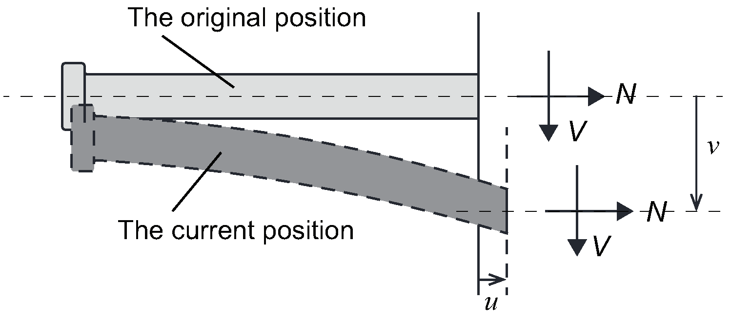
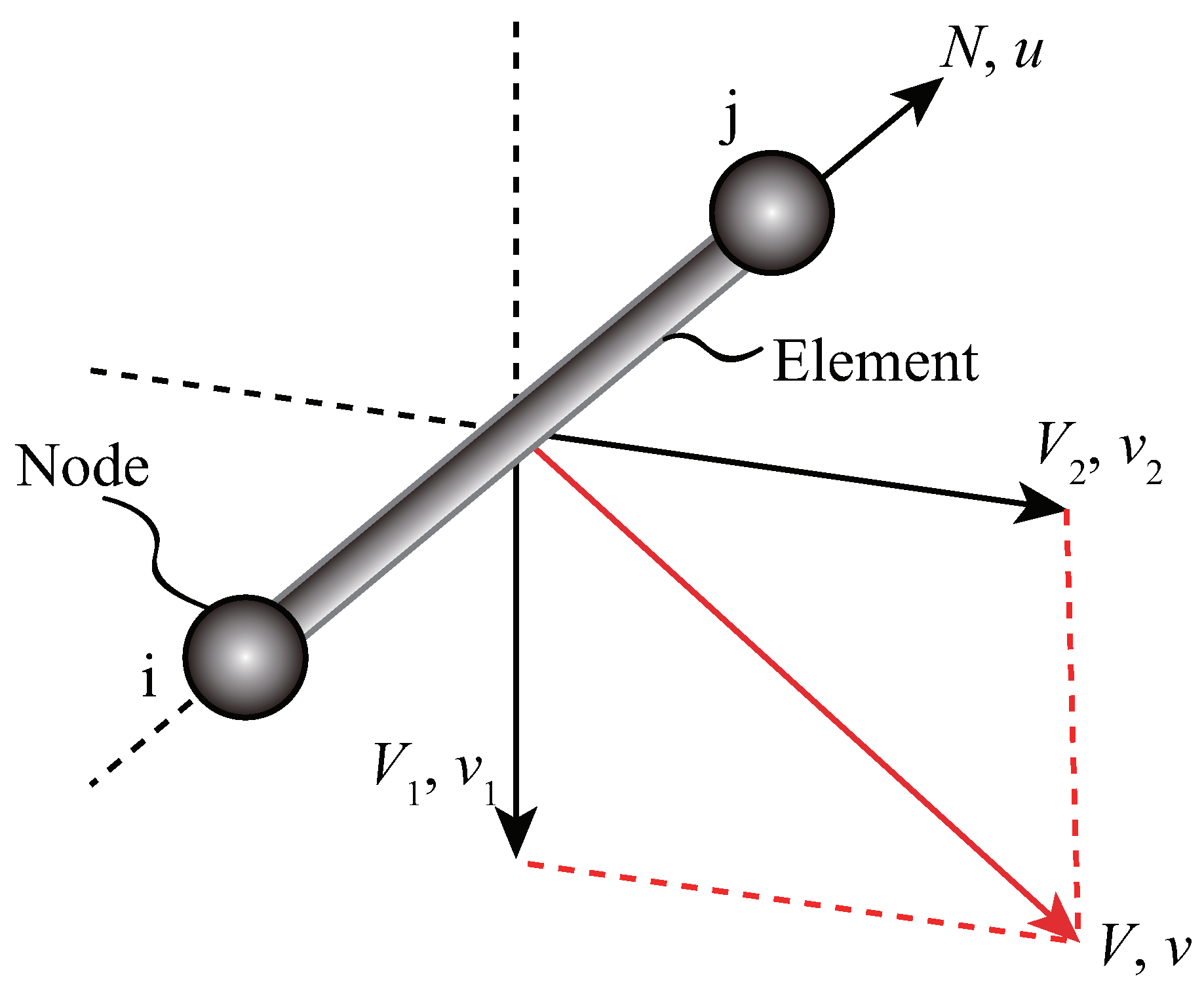
Positioned at the intersection between the steel beam and concrete slab, the stud connector is subjected to diverse permutations of vertical and horizontal movements under the simultaneous impacts of shear and tension, subsequently engendering a complex stress state. The meticulously defined macroscopic elastoplastic constitutive model successfully captures the response of the stud connection through defining the relationship between the force vector, denoted as , and the relative interface displacement vector, denoted as . This relationship, designated in-plane, is hereinafter referred to as the load–displacement correlation. The definitions of and imply that the composite response of both the stud connector and the adjoining reinforced concrete are implicitly encapsulated within the model. This observation further dictates that any variations—be they material properties or geometrical nuances—within either constituent of the stud connection exert a significant influence on the parameters of this model. The directions of the net positive force and the consequent relative displacement at the steel–concrete interface resulting from the forward force can be inspected in Figure 1. Given this backdrop, it is indeed pertinent to define and in the following manner:
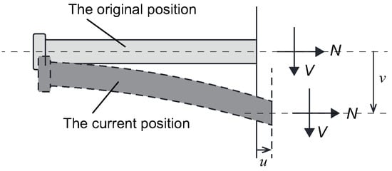
Figure 1.
Positive direction of forces and displacements.
Attention should be directed to the fact that within this paper, variables presented in bold typeface consistently signify vectors or matrices.
In the context of capturing the nonlinear behavior of stud connections under the synergistic influence of shear and tensile loads, the macroscopic elastoplastic model is primarily composed of the following elements:
- (1)
- An empirical formulation of the yield surface within the force plane, labeled as . This is achieved by delineating the contour of the yield surface, which is informed by the shape of the failure envelope;
- (2)
- A strain hardening scheme that elucidates the functional interrelation between the magnitude of the yield surface and the plastic deformation. The expansion of the yield surface is a function of the evolution of plastic displacement (where ). The extent to which the yield surface expands is quantified by the shear force that corresponds to a given plastic displacement;
- (3)
- An aptly chosen flow rule that enables the prediction of increments in plastic displacement, denoted as , which results from the yield surface’s dilation or constriction.
- (4)
- An elastic load–displacement relationship is employed to delineate the load–displacement behavior that occurs within the confines of the yield surface.
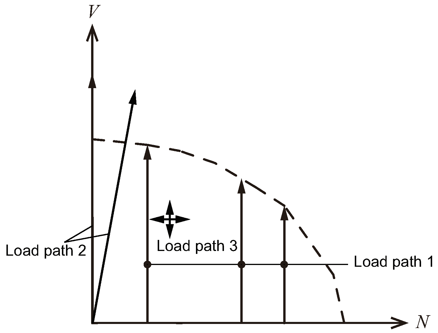
The acquisition of the components integral to the above-outlined elastoplastic model mandates the undertaking of an adaptation process. This process involves fitting expressions, representative of these components, to data derived either experimentally or through the deployment of finite element simulations. This article espouses the utilization of three distinct loading paths, which serve to offer ancillary data support pivotal to the fabrication of the elastoplastic model. These chosen trajectories are illustrated in Figure 2:
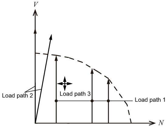
Figure 2.
Load path diagram.
- (1)
- Load path 1: shear direction loading under different drawing force levels. The shape enclosed by the extremities of the load path may be posited as depicting the trajectory of the yield surface which is apt for the elastoplastic model. This load path is instrumental in deducing both the hardening rule and the flow principle inherent to the elastoplastic material model;
- (2)
- Load path 2: radial loading. These loading trajectories inform the hardening principle as well as the flow rule characteristic of the elastoplastic model. The instance of pure shear loading does indeed represent a specific case within this load path, from which the shear–slip hardening principle applicable to the stud connection can be extrapolated;
- (3)
- Load path 3: elastic stiffness test. By introducing minimal displacements in both planar directions while concurrently unloading the stud connection, it is feasible to establish an estimation of the elastic stiffness coefficient.
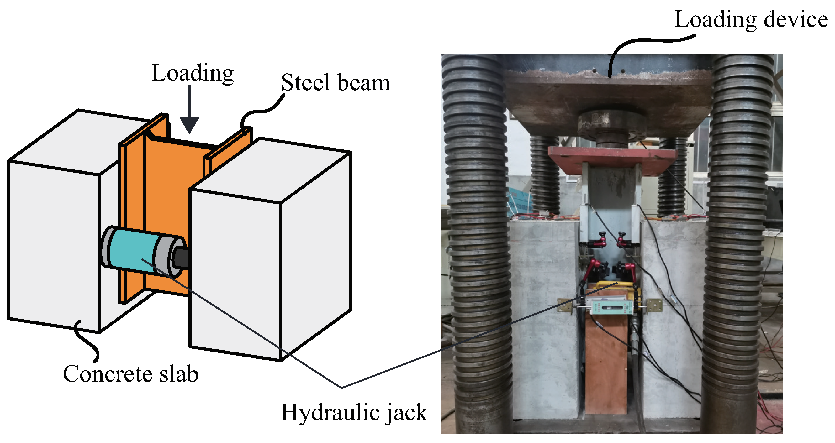
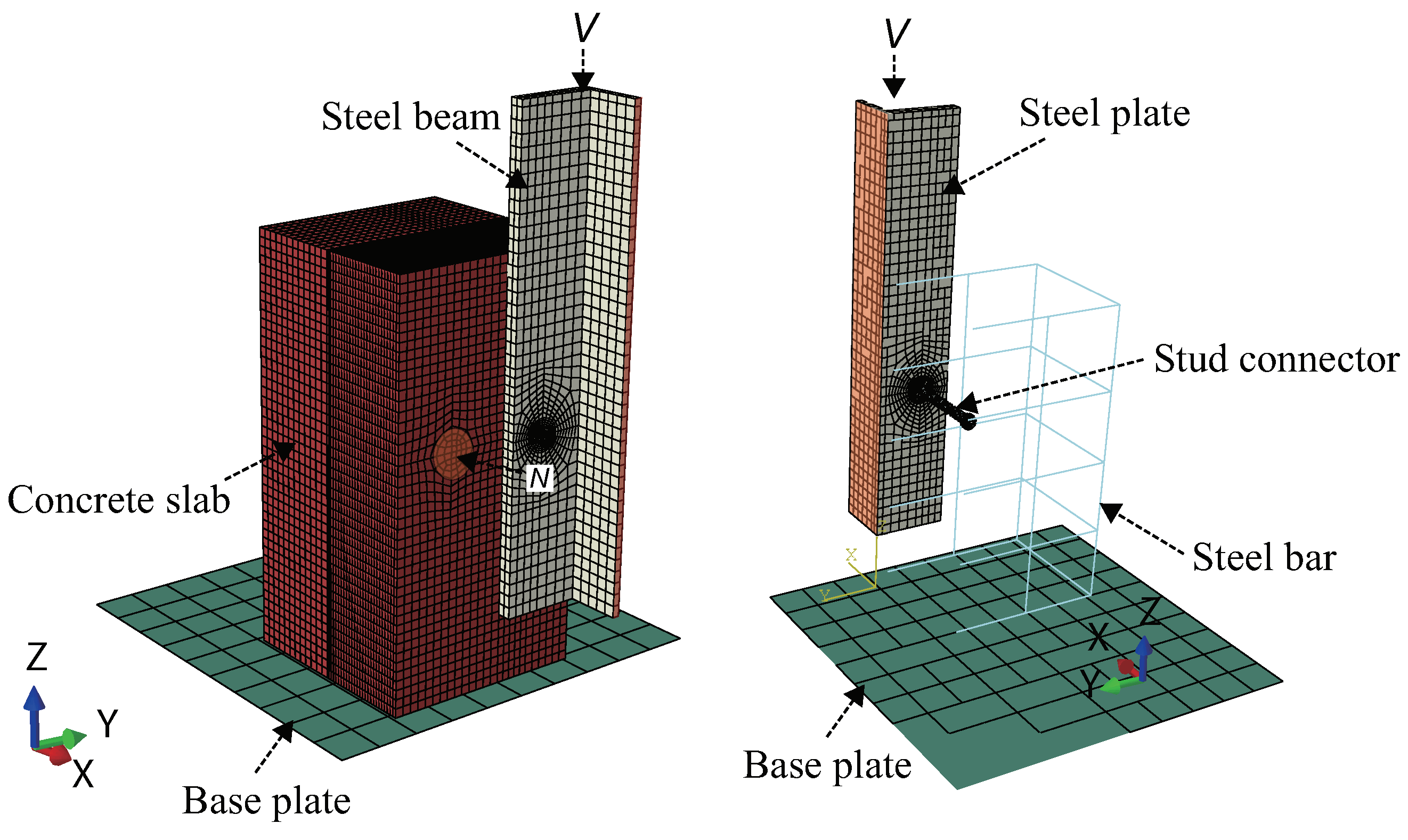
To this end, a series of push-out tests on stud connections were conducted, using the test setup depicted in Figure 3. The employed configuration incorporated a hydraulic jack positioned between the concrete slabs designated to impose tensile stress upon the stud connections, extending along with a separate jack linked to the reaction frame to exert shear forces. The mutable parameters within the push-out test specimens included the elastic modulus of the concrete, the diameter of the stud, and the intensity of the applied tensile force onto the stud. The shear–slip curve under different tensile forces was thus obtained through these tests for the stud connections. Subsequently, a finite element modeling approach was implemented to simulate the push-out tests under shear load for the stud connections, using the finite element model shown in Figure 4. The finite element method empowered us to imitate a broader spectrum of loading paths and engage in parametric analysis. This occasioned an intensive exploration into the ramifications of variables such as the length and diameter of the stud, the elastic modulus of both the concrete slab and the stud, and the volume ratio of reinforcement. Whilst a summary of the elastoplastic model is present, a more comprehensive breakdown of the push-out tests and the finite element models is available in the cited work [41].
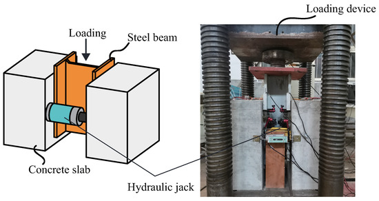
Figure 3.
Setup of push-out test.
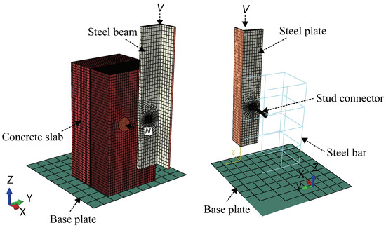
Figure 4.
Finite element model of push-out test.
3. Details of the Model
3.1. Elastic Behavior
The elastic stiffness inherent in the stud connection constitutes a critical facet of its associated elastoplastic model. In the pursuit of computing any load or displacement increment occurring within the yield surface, it is imperative to furnish a characterization of the stud connection’s elastic response. The elastic relationship between the increment of force and the corresponding increment of elastic displacements can be expressed as follows:
where represents the elastic stiffness matrix, and denote the elastic tensile and shear stiffness, respectively, and is the coupling stiffness.
The elastic stiffness matrix is obtained by fitting the result of the finite element simulation of the stud connections under load path 3 [41], and it can be expressed as follows:
where , , and are the stud diameter, the elastic modulus of the concrete, and the elastic modulus of the stud, respectively.
3.2. Yield Surface
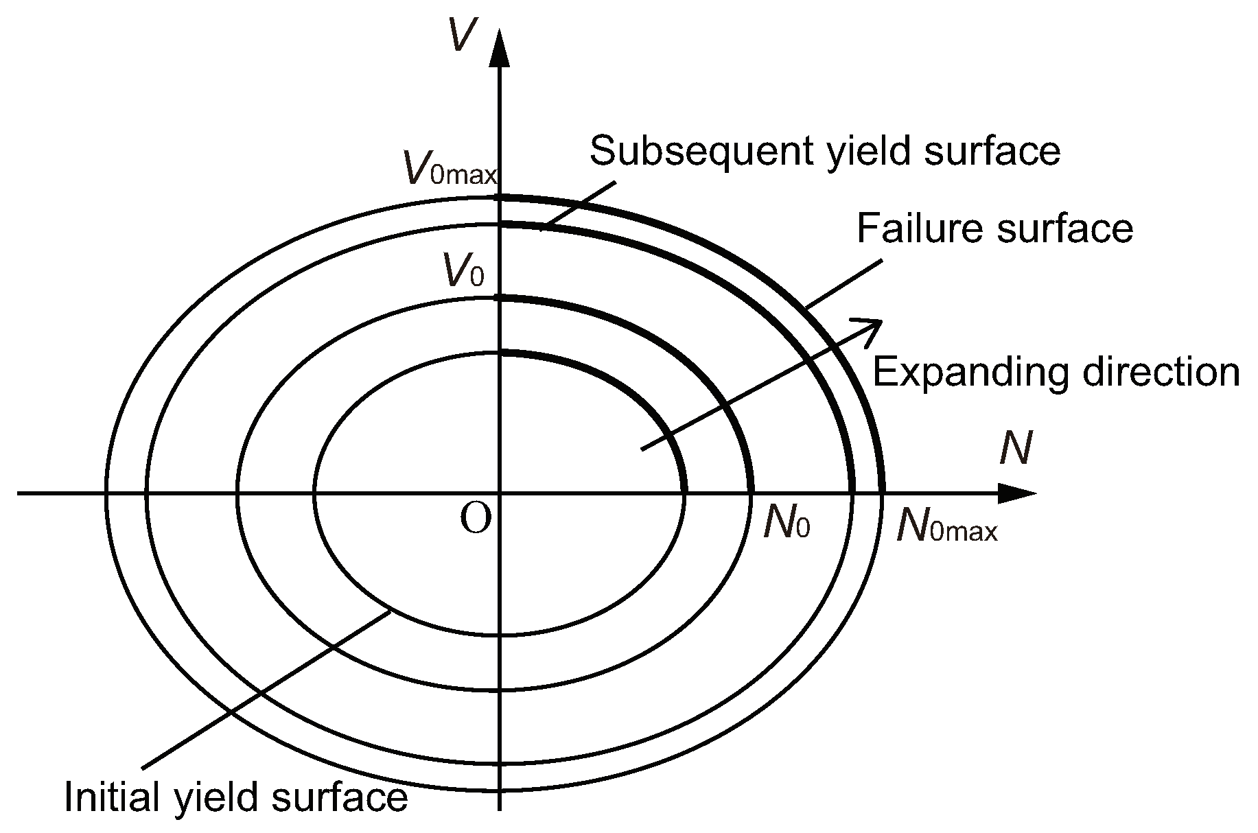
The demarcation between the purely elastic and the combined elastic–plastic states is referred to as the yield surface. Specifically identifying the first transition from an elastic to an elastoplastic state, the defined yield surface can be called the initial yield surface for the stud connection. As the loading process progresses, this initial yield surface undergoes a constant expansion, generating what can then be described as the subsequent yield surface. Bringing this process to conclusion, when the connection attains its point of failure, the yield surface present at that juncture is coined the failure surface. Figure 5 provides a graphic representation of these stages, displaying schematic outlines of the initial yield surface, the subsequent one, and, ultimately, the failure surface. Regarding the shape of the failure surface, established experimental data and data from finite element simulations [42,43,44,45] have collectively affirmed that it approximates to the envelope of a convex arch. On this evidence, we can represent the failure surface through an equation that captures the form of such a convex envelope.
where and are the radius of the horizontal and vertical axes of the failure surface, respectively, and is the aspect ratio defining the surface shape. The initial path of the yield surface in the () load plane can be obtained by shrinking the shape of the failure surface as follows:
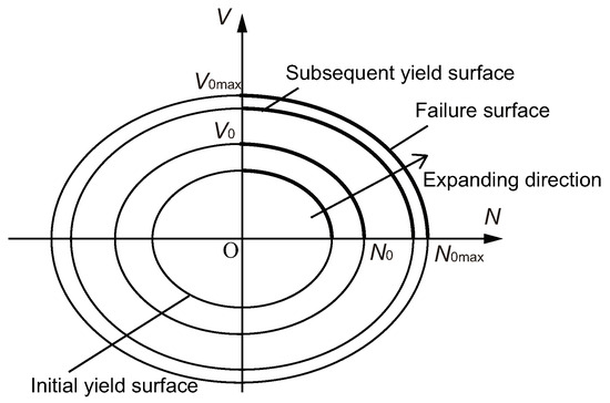
Figure 5.
Yield surface diagram.
In order to derive the mathematical expressions for both the failure surface and the initial yield surface, as denoted in Equations (5) and (6), it is imperative to ascertain the formulae for the characteristic parameters , , , and . The values of these parameters are deduced by fitting them to the empirical outcomes obtained from push-out tests, as well as the results from finite element simulations corresponding to load path 1, as documented in the study by Qin [41]:
Presuming that the morphology of the subsequent yield surface mirrors that of both the initial yield surface and the failure surface, we can formulate the subsequent yield surface. This is achieved by implementing an expansion of the initial yield surface, specified as follows:
The size of the yield surface is represented by , the shape of the yield surface is determined by (), and the centroid of the yield surface is ().
3.3. Hardening Law
Building on the hypothesis that an augmentation in plastic displacement within the shear dimension contributes to the expansion of the yield surface, the size of the yield surface when the system is in a pure shear state is dictated by the principles of isotropic hardening. The isotropic hardening law delineates the interdependence of the shear force and the plastic slip pertinent to the shear direction in the stud connectors. To encapsulate this, we draw on the shear–slip correlation derived from the insights of push-out tests complemented by finite element analysis simulations. The equation representing this correlation is:
Further, the relation between the shear force and the plastic slip in the shear direction of the stud connection during the elastic–plastic stage is
where represents the cumulative outcome of integrating the incremental plastic displacements along the shear vector. Drawing from the empirically derived shear–slip response curves of the push-out tests under pure shear conditions, as documented by Qin [41], a functional relationship is established between the shear force and the total slip v. To isolate the plastic component, one subtracts the elastic part from the total slip v, thereby obtaining the plastic slip . By differentiating the shear force with regard to the plastic slip , we arrive at a differential equation that articulates the dynamic interplay between the shear force and the plastic slip within the realm of the shear direction:
Although Equation (11) might be sufficient to fit the shear–slip curve, it does not account for complex loading conditions that entail plastic displacement in both the shear and tensile directions simultaneously. To account for the influence of plastic displacement in the tensile direction on the size of the yield surface , an alternative methodology is necessary. To maintain consistency with the hardening law for both the pure shear and shear–tensile states, a new parameter called the plastic displacement strength, denoted as , is introduced to replace in the formula when the stud connection experiences plastic displacement in both the shear and tensile directions, namely
The plastic displacement strength is a function of the plastic displacement in the shear direction and the plastic displacement in the tensile direction, which can be obtained by integrating the plastic displacement increments and , respectively. It is crucial to ensure the hardening law observed in the shear–tensile states aligns seamlessly with that strictly within the pure shear domain. To discern the dimensions of the yield surface, one must compute the value of as derived from the vertical plastic displacement during a pure shear state. Under shear–tensile conditions, equates to . This conclusion can be reached by replacing the corresponding values of and at any point on the yield surface with . By adhering to these guiding principles, one can acquire the optimally fitted value for Equation (12) as follows:
3.4. Flow Rule
The increase in plastic displacement at yield defines an appropriate flow rule. The flow rule within the two-dimensional () load plane is informed by load paths 1 and 2, and a non-associated flow criterion espoused by the elastoplastic stud connection model is exhibited [41]. To model the interplay between load and incremental displacement, it becomes requisite to charter an expression for the plastic potential g, which retains its identity distinct from the yield surface. Herein, our focus shifts to presenting a formulation for the plastic potential, one that mimics the equation for the yield surface closely, but introduces modifications at the apex and shape of the plastic potential surface. This adaptation is enabled using plastic potential parameters , , and . Consequently, the equation delineating the plastic potential can be articulated as follows:
where is the maximum shear value of the plastic potential at the present time, which is similar to in the expression of the yield surface. By regulating the parameters and , one can subtly alter the form of the plastic potential surface.
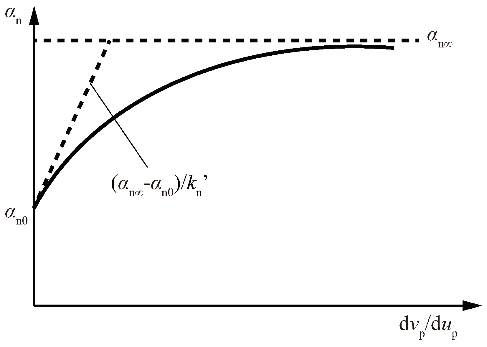
The ideal values of fluctuate in accordance with the varying ratios of plastic displacement iterations . To uphold the flow rule’s consistency across an assortment of values, this nuance must be carefully addressed. To accurately emulate this dynamic, an escalation in is required as increases, highlighting an intensified degree of non-associated flow. One can chart the fluctuation pattern of employing hyperbolic functions. In this context, the plastic displacement iteration , as observed in the shear direction, is rendered normalized by the corresponding plastic displacement iteration within the tensile direction:
where represents the parameter value of with no increase in plastic displacement, represents the limiting value attainable by the parameter, and represents the rate at which attains its limiting value . Figure 6 depicts the evolution of . The impact of fluctuating values on the theoretical prediction curve is depicted in Figure 7: During the initial timeframe at point A, where , a compelling proximity is observed between the experimental and finite element results in conjunction with the theoretical prediction curve. With load application, the experimental and finite element outcomes progressively gravitate towards the theoretical prediction curve, under circumstances of . The pace of this transition is dictated by the expansion rate of the plastic potential surface, which, in turn, is determined by .
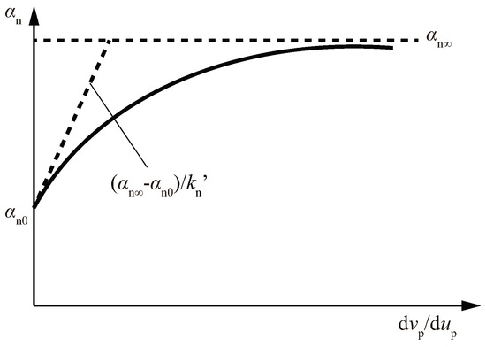
Figure 6.
The relationship between and .
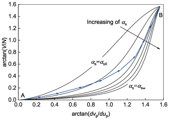
Figure 7.
The theoretical prediction curves with different values of .
Equation (14) articulates the theoretical variations in the plastic displacement within both the shear and tensile directions:
where can be derived from the consistency condition intrinsic to the strain hardening law. The enhancement observed in the plastic displacement ratio can be represented through an expression relevant to the current state:
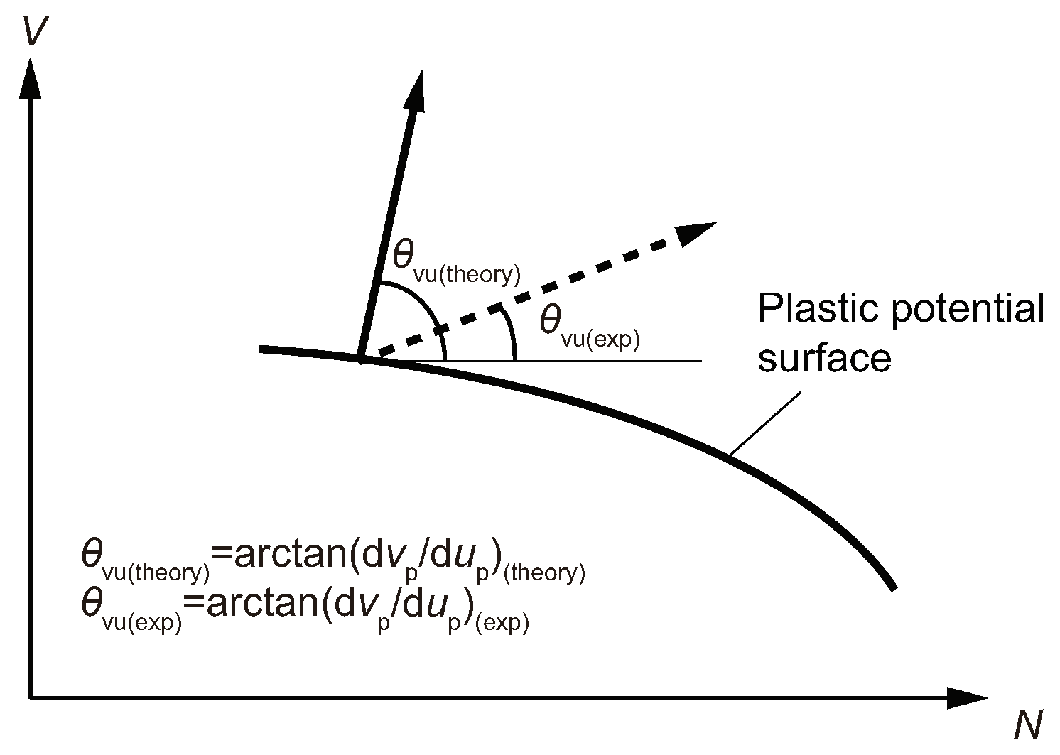
As depicted in Figure 8, the angle signifies the direction of the theoretical plastic displacement increment, as calculated by Equation (18). On the other hand, characterizes the direction of the plastic displacement increment, as derived from experimental and finite element simulation results. In seeking a fit between and , the values of the parameters intrinsic to the flow rule emerge as follows: = 1.69, = 1.00, = 2.40, and = 3.00 [41].
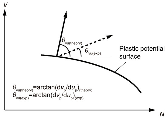
Figure 8.
The definition of the plastic displacement increment angle.
To calculate the size of the plastic potential surface (i.e., the size of ), the parameter is defined. The size of x is obtained by the following numerical solution:
4. Constitutive Integration Algorithm
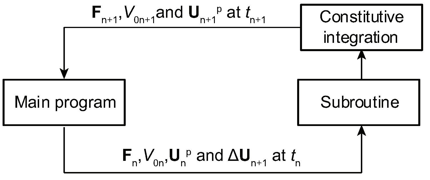
The elastoplastic behavior of stud connections can be represented through integration with a macroelement, which directly delineates the force–displacement interactions specific to stud connections. This macroelement can be effortlessly integrated into the comprehensive finite element analysis of the structure as a cohesive component. To aid in the customization of macroelement characteristics, Abaqus offers a User Element Subroutine (UEL) [46]. The load–displacement curve of the elastoplastic model is encapsulated within this user-defined subroutine. The initial load and the plastic state variable at time are passed to the subroutine by the primary analysis program. Upon receiving the displacement increment , the subroutine is tasked with computing the subsequent load and plastic state variable at the conclusion of the interval using the constitutive integral method, and then relaying these results back to the main program. This symbiotic exchange between the main program and the subroutine is graphically represented in Figure 9.

Figure 9.
The interaction between the main program and the subroutine.
Prior to constitutive integration, it is assumed that the plastic state variables remain unchanged ( = 0, = 0) after loading :
This phase is commonly referred to as the elasticity prediction since the trial load is derived, presuming solely elastic behavior. Within each incremental step, the trial load is assessed, utilizing either the pure elastic or elastoplastic formulation depending on the load step’s termination condition. Five potential scenarios (depicted in Figure 10) are employed to establish the position of the loading state in relation to the currently defined yield surface:
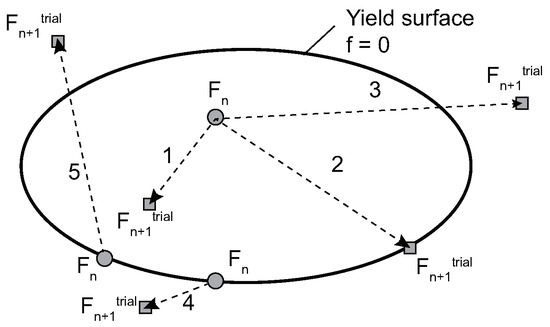
Figure 10.
Possible cases of the loading state.
Case 1: If , it suggests that the test load resides within the yield surface; hence, an elastic increment should be implemented. The trial load state, , is deemed the final load state. Thus, is recognized as the actual force , and the value of should be set as :
Case 2: If , it signifies that the test load exactly falls on the yield surface. Similarly, an elastic increment is prescribed, and the trial load state is finalized. Here again, embodies the actual force , and is assigned to .
Cases 3, 4, and 5: When , this signifies that the test load is located outside the current yield surface, and, thus, plastic behavior is expected. The constitutive equation will need to integrate the displacement increment:
Hence, the primary aim of the constitutive integration is to determine the plastic displacement increment in cases 3, 4, and 5. This research utilizes the backward Euler method for integration [47], which is recognized for being an implicit algorithm. The selection of the backward Euler method is attributed to its computational efficiency and robust theoretical foundation. It is especially beneficial for addressing highly nonlinear issues due to its inherent stability, straightforwardness, and ease of implementation. The implicit algorithm sets out to compute the plastic displacement increment and the plastic state variable , beginning from the trial load’s final state , and adjusts the load state back to the yield surface at . Throughout the iteration process, it carries out constitutive integration based on the increment’s final state and calculates the load at the increment’s conclusion.
The plastic multiplier and the differential of plastic potential energy in the equation are evaluated using the state at the end of the increment.
As demonstrated in Equation (23), an iterative process is needed to navigate the test load back to the yield surface. In the context of the elastoplastic model, , , and should concurrently satisfy the conditions on the updated yield surface. Consequently, alongside Equation (23), it becomes crucial to perform integration in accordance with the hardening law to derive the revised plastic state variable:
In addition, at the end of the step, the yield condition should be applied:
By defining the residual , Equations (23)–(25) can be solved by the Newton–Raphson iterative method. In essence, through iteration, the load, displacement, and state variables adhere to the equation of the yield surface, flow rule, hardening law, and consistency condition:
The above equation solution of ) can be obtained through iteration, until the residual , and is the allowable error. The iterative procedure is as follows:
In the formula, is the Jacobian matrix of the above nonlinear Equation, (26), which is a square matrix.
To improve the clarity and understanding of the integration algorithm process, a detailed flow diagram was constructed, as illustrated in Figure 11.
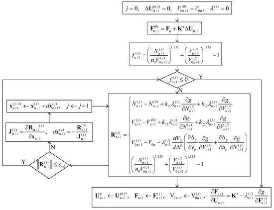
Figure 11.
Process of the integration algorithm.
5. Continuum and Consistent Tangent Stiffness
The fundamental approach for addressing nonlinear finite element problems is through Newton–Raphson iteration. A crucial step in implementing this iterative method for finite elements is calculating the tangent stiffness matrix, which characterizes the relationship between force and displacement gradients based on the current force and displacement states.
5.1. Continuum Tangent Stiffness
The conventional tangent stiffness method usually adopts the continuum elastic–plastic tangent modulus. For the incremental load–displacement relationship of pure elasticity, its expression is
The expression of the elastoplastic incremental load–displacement relationship is
where is the elastoplastic stiffness matrix, also known as the continuum elastoplastic tangent modulus.
If the load increment remains entirely within the yield surface, the elastic displacement can be determined using Equation (3). Upon yielding, the increment vector of plastic displacement, , is oriented perpendicularly to the plastic potential surface. The magnitude of the plastic displacement increment, , is defined by the scaling factor ,
Whenever there is an increment in load or displacement that crosses the yield surface, the variation in the value of f for the yield function must be zero (i.e., ) to ensure that the load point, characterized by the normal force N and shear force V, remains on the yield surface. In accordance with the strain hardening rule, a solution for must exist signifying that a certain magnitude of plastic displacement is achievable which fulfills the yield criterion
where and depend on the plastic displacement strength . According to the chain rule and the plastic potential relationship, Equation (31) can be written as
Therefore, the solution of can be obtained from the consistency condition,
5.2. Consistent Tangent Stiffness
The Newton–Raphson iterative method is characterized by a second-order rate of convergence. However, when applied to the computations of the continuum elastic–plastic tangent modulus , the backwards Euler method generally achieves only first-order accuracy. This results in a discrepancy between and the updating format of the path-independent variables. Consequently, the Newton–Raphson iterative technique cannot guarantee a quadratic convergence rate. To ensure the second-order convergence rate of the tangent stiffness method, it is necessary to devise an updating scheme for path-independent variables that yields first-order precision, aligning it with a consistent elastoplastic tangent modulus [48]. Moreover, in finite element analysis, it is crucial to define to derive the Jacobian matrix essential for equilibrium iteration. is defined as
where is the force increment and is the displacement increment. We know that
so Equation (35) can be written as
where
in which denotes a () identity matrix and denotes a () matrix with zeros. To obtain , we reformulate Equation (26) as
6. Finite Element Formulation
While defining the macroelement through the User Element Subroutine (UEL), the structure of a two-node element is adopted. These two nodes might either coincide or possess a certain distance between them. For the purpose of this explanation, we designate these nodes as i and j. As a result, the displacement increment function vector for the element, denoted as , can be construed as follows:
and the vector of force increment function for the element is
The strain–nodal displacement parameter relation of the element is
in which L is the length of the element; is the strain–displacement transformation matrix given by
According to the constitutive relations, the stress vector of the element could be written as
where A denotes the cross-section area of the element.
Considering the element contribution to the equilibrium of the system, the nodal forces that the element provides are
in which V is the volumn of the element, is the shape function of the element, and is the volume force increment. No volume force is considered in this element, so the equation could be written as
One integration point is adopted and the weight factor is one. Substituting Equations (45) and (47) into Equation (49) results in
Thus, the element stiffness is
7. Application and Validation
7.1. Application of Integration Algorithm
The efficacy of the elastoplastic constitutive model is substantiated through a numerical illustration. This instance makes use of a singular macroelement force-resultant model (as demonstrated in Figure 12). This study sought to scrutinize the influence of allowable errors, denoted as , amidst the application of the backward Euler integration scheme, particularly with respect to computational precision and efficiency.

Figure 12.
The single macroelement model in Abaqus.
In this example involving a single macroelement, the stud’s diameter was established at 16 mm, with the concrete’s compressive strength for a cubic sample measured at 54.06 MPa. The elastic modulus for concrete was set at 35,188 MPa, and for steel, it was 206,000 MPa. The stud’s tensile strength was identified as 496.79 MPa. This numerical demonstration utilized displacement loading, where the axial and shear directions underwent proportional radial loading until reaching a predetermined displacement threshold. The analysis procedure was segmented into 1000 incremental steps, with each step approximating a 0.007 mm increment in the shear direction. Throughout the analysis, the peak incremental step number was capped at 10,000, starting with an initial step size of 0.001. The step size ranged from a minimum of to a maximum of . Various allowable error thresholds , including 1, , , , and , were employed for the calculations. The backward Euler integration method is theoretically capable of delivering precise integration outcomes, with smaller allowable errors yielding more accurate results. Consequently, a scheme adopting an allowable error of was considered to approach the exact solution most closely.
Figure 13 presents the anticipated load relation curves alongside the load–displacement curves for various integration methods with differing error tolerances . Observations from Figure 13 reveal that within the framework of the backward Euler integration method, setting to one leads to a marked divergence of the calculated results from the precise solution. This discrepancy arises due to the substantial tolerance level failing to adequately amend the elastic forecast in proximity to the yield surface. However, when the allowable error is reduced to or less, the computed outcomes demonstrate high fidelity to the exact solution.
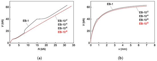
Figure 13.
Computational results. (a) Load relation curve. (b) Load–displacement curve.
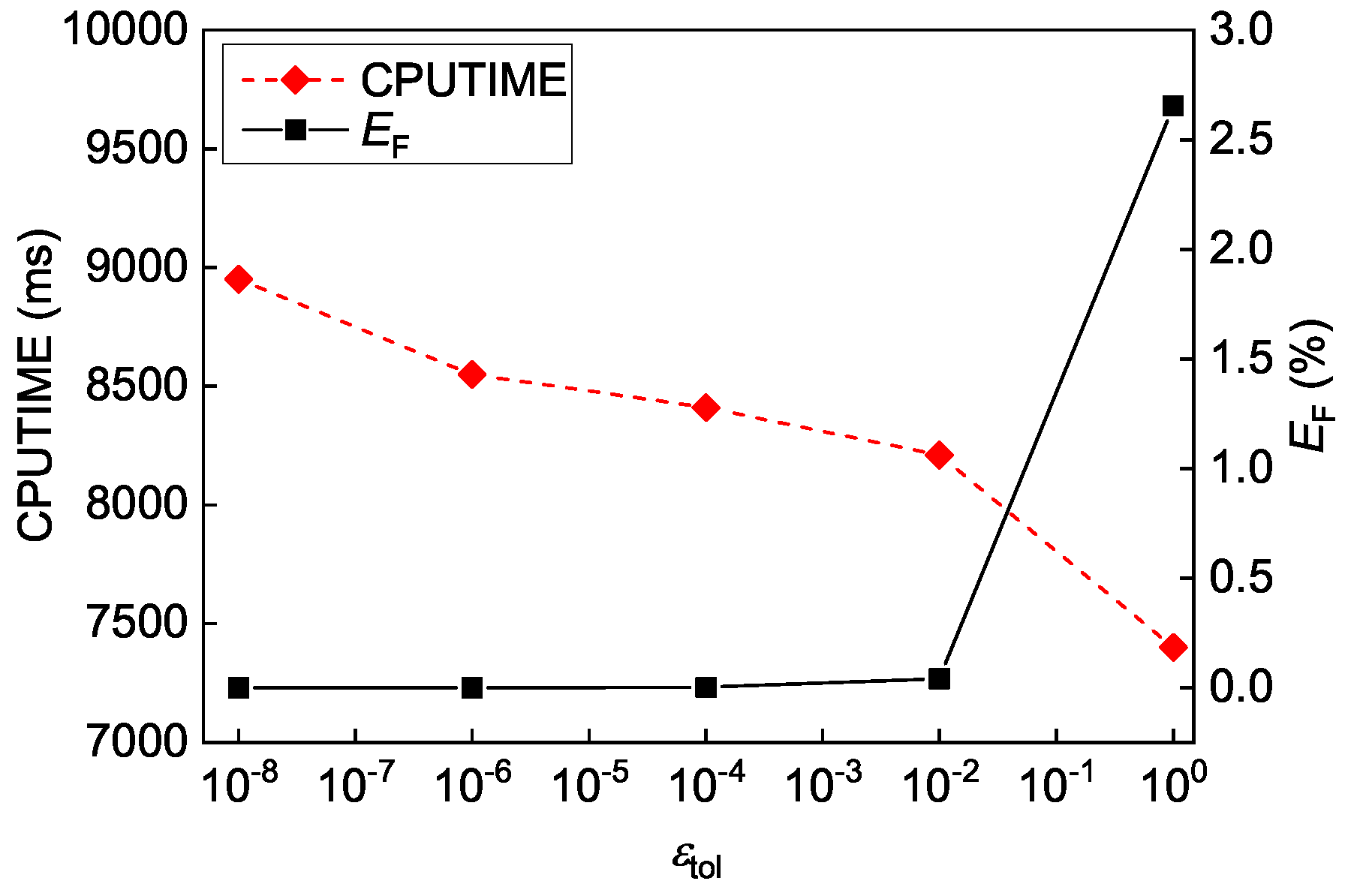
To assess the effectiveness of an integration procedure, two statistical indicators can be employed: and CPUTIME. The computation of the maximum discrepancy in the load for the designated integration process is conducted as detailed below:
where represents the integration load for each respective integration procedure, while serves as the reference load. In this specific case, the computational outcomes derived from the backward Euler method, under an error tolerance set at = , are utilized as the baseline load. CPUTIME indicates the execution time of the integration procedure. When the computational duration for a single macroelement is notably brief, augmenting the number of iterations may contribute to a more precise evaluation of CPUTIME.
Developing a graph of CPUTIME and against as demonstrated in Figure 14 can provide a visual representation of the integration procedure’s accuracy and efficiency. One can observe that CPUTIME remains largely unvaried in response to changes in . Furthermore, the backward Euler integration method, often regarded as theoretically unconditionally stable [48,49,50], renders robust and efficient performance, even when values are minimized. This algorithm’s output leans towards convergence without being overly sensitive to predetermined assumptions. However, employing the implicit backward Euler integration within the realm of elastoplastic models necessitates that displacement increments should be maintained in comparatively small sizes to assure convergence. Additionally, executing the implicit algorithm involves greater technical complexity, and introducing kinematic hardening criteria into the elastoplastic model further escalates the numerical computation complexity.
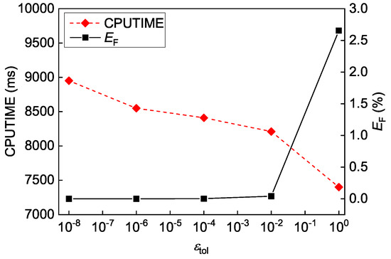
Figure 14.
Comparison CPUTIME and for different .
7.2. Validation by Experimental Results
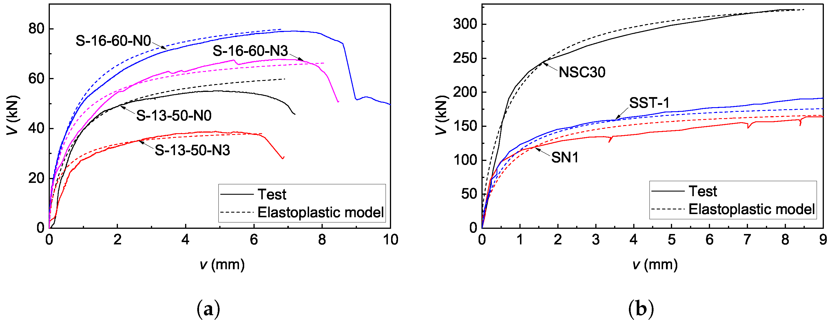
To affirm the efficacy of the proposed elastoplastic model for stud connections in accurately predicting load–displacement curves, this study leverages data from push-out tests documented in various research efforts for model validation. Interested readers can refer to the specified publications [41,45,51,52], for detailed experimental data and methodologies. The chosen material properties and geometric parameters mirror those outlined in several referenced studies. An ABAQUS data file was meticulously prepared, and the UEL subroutine, embodying the elastoplastic model, was invoked to simulate the shear force–displacement behavior of the samples. Displayed in Figure 15, the results illustrate that the shear force–displacement curves generated by the elastoplastic model for stud connections closely align with both the experimental and finite element analysis findings, validating the model’s capability to accurately predict the load–displacement behavior of monotonically loaded stud connections. Nonetheless, it is important to note that the model falls short of predicting the descending portion of the load–displacement curve.
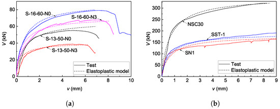
Figure 15.
Verification of the proposed elastoplastic model. (a) First set of data. (b) Second set of data.
8. Conclusions
This research presents a significant advancement in the design and analysis of composite structures by introducing a macroscopic elastoplastic constitutive model for stud connections. The development of this model is rooted in plasticity theory and is informed by empirical data derived from push-out tests as well as finite element simulations. Our results demonstrate that by integrating the combined effects of shear and tensile forces, the model offers a more accurate prediction of the load–displacement behavior of stud connections, which is paramount for ensuring structural integrity and safety.
The comparative analysis with experimental push-out test data revealed that the elastoplastic model offers superior predictive capabilities over traditional models based on nonlinear elastic theory. This highlights the importance of considering elastoplastic effects to more realistically capture the complex behavior of stud connections, especially under conditions that induce plastic deformation. By doing so, the proposed model addresses the limitations of previous models, enabling a more precise analysis of structural stiffness and load-bearing capacity. This precision is crucial for the internal redistribution of forces and the accumulation of plastic damage, which are critical factors in the longevity and safety of composite structures.
Moreover, the numerical example implemented in ABAQUS demonstrated the model’s stability and robustness, suggesting that the model can be effectively utilized in practical engineering applications. The implementation of the backward Euler method ensures the accuracy of the solution and the consistency of the tangent stiffness necessary for the convergence of the nonlinear finite element analysis.
In conclusion, the macroscopic elastoplastic constitutive model proposed in this study is a substantial contribution to the field of composite structure analysis. It not only enhances the accuracy of predictions concerning the performance of shear connections but also serves as a reliable tool for engineers to design safer and more efficient structures. Future work may extend the application of this model to more complex loading scenarios and explore its integration into broader structural analysis frameworks, thereby reinforcing its value to the engineering community.
Author Contributions
Conceptualization, X.Q. and W.Z.; methodology, X.Q.; software, X.Q.; validation, X.Q. and W.Z.; formal analysis, X.Q.; investigation, W.Z.; resources, W.Z.; data curation, X.Q.; writing—original draft preparation, X.Q.; writing—review and editing, X.Q.; visualization, W.Z.; supervision, W.Z.; project administration, X.Q.; funding acquisition, X.Q. All authors have read and agreed to the published version of the manuscript.
Funding
This research was funded by the general scientific research project of the Zhejiang Education Department (No. Y202250036).
Data Availability Statement
Data available on request due to privacy.
Acknowledgments
The authors wish to express their thanks for the financial assistance.
Conflicts of Interest
The authors declare no conflicts of interest.
References
- Akbas, S.D. Nonlinear behavior of fiber reinforced cracked composite beams. Steel Compos. Struct. 2019, 30, 327–336. [Google Scholar]
- Aklilu, G.; Adali, S.; Bright, G. Failure analysis of rotating hybrid laminated composite beams. Eng. Fail. Anal. 2019, 101, 274–282. [Google Scholar] [CrossRef]
- Lu, B.; Zhai, C.; Li, S.; Ji, D.; Lu, X. Influence of Brittle Fracture of Shear Connectors on Flexural Behavior of Steel–Plate Concrete Composite Beams Under Cyclic Loading. Int. J. Steel Struct. 2020, 20, 1703–1719. [Google Scholar] [CrossRef]
- Zhang, Y.; Liu, A.; Chen, B.; Zhang, J.; Pi, Y.L.; Bradford, M.A. Experimental and numerical study of shear connection in composite beams of steel and steel-fibre reinforced concrete. Eng. Struct. 2020, 215, 110707. [Google Scholar] [CrossRef]
- Lima, J.M.; Bezerra, L.M.; Bonilla, J.; Barbosa, W.C. Study of the behavior and resistance of right-angle truss shear connector for composite steel concrete beams. Eng. Struct. 2022, 253, 113778. [Google Scholar] [CrossRef]
- Lawson, R.M.; Taufiq, H. Partial shear connection in light steel composite beams. J. Constr. Steel Res. 2019, 154, 55–66. [Google Scholar] [CrossRef]
- Jiang, H.; Fang, H.; Liu, J.; Fang, Z.; Zhang, J. Experimental investigation on shear performance of transverse angle shear connectors. In Proceedings of the Structures; Elsevier: Amsterdam, The Netherlands, 2021; Volume 33, pp. 2050–2060. [Google Scholar]
- Wang, Y.H.; Yu, J.; Liu, J.P.; Chen, Y.F. Shear behavior of shear stud groups in precast concrete decks. Eng. Struct. 2019, 187, 73–84. [Google Scholar] [CrossRef]
- Kim, S.E.; Papazafeiropoulos, G.; Truong, V.H.; Nguyen, P.C.; Kong, Z.; Duong, N.T.; Pham, V.T.; Vu, Q.V. Finite element simulation of normal–Strength CFDST members with shear connectors under bending loading. Eng. Struct. 2021, 238, 112011. [Google Scholar] [CrossRef]
- Wei, X.; Xiao, L.; Pei, S.L. Shear behavior of multi-hole perfobond connectors in steel-concrete structure. Struct. Eng. Mech. 2015, 56, 983–1001. [Google Scholar]
- Zheng, S.J.; Liu, Y.Q.; Yoda, T.; Lin, W.W. Shear behavior and analytical model of perfobond connectors. Steel Compos. Struct. 2016, 20, 71–89. [Google Scholar] [CrossRef]
- Ataei, A.; Zeynalian, M.; Yazdi, Y. Cyclic behaviour of bolted shear connectors in steel-concrete composite beams. Eng. Struct. 2019, 198, 109455. [Google Scholar] [CrossRef]
- Zhai, C.; Lu, B.; Wen, W.; Ji, D.; Xie, L. Experimental study on shear behavior of studs under monotonic and cyclic loadings. J. Constr. Steel Res. 2018, 151, 1–11. [Google Scholar] [CrossRef]
- Chiniforush, A.A.; Ataei, A.; Bradford, M.A. Experimental study of deconstructable bolt shear connectors subjected to cyclic loading. J. Constr. Steel Res. 2021, 183, 106741. [Google Scholar] [CrossRef]
- Nie, J.; Tang, L.; Cai, C. Performance of steel-concrete composite beams under combined bending and torsion. J. Struct. Eng. 2009, 135, 1048–1057. [Google Scholar] [CrossRef]
- Lin, W. Study on steel-concrete composite beams under pure negative bending and combined negative bending and torsion. In Proceedings of the IABSE Conference, Kuala Lumpur 2018: Engineering the DevelopingWorld. International Association for Bridge and Structural Engineering (IABSE), Kuala Lumpur, Malaysia, 25–27 April 2018; pp. 103–110. [Google Scholar]
- Rehman, N.; Lam, D.; Dai, X.; Ashour, A. Testing of composite beam with demountable shear connectors. Proc. Inst. Civ. Eng. Struct. Build. 2018, 171, 3–16. [Google Scholar] [CrossRef]
- Tan, E.L.; Uy, B. Experimental study on curved composite beams subjected to combined flexure and torsion. J. Constr. Steel Res. 2009, 65, 1855–1863. [Google Scholar] [CrossRef]
- Lin, Z.; Liu, Y.; He, J. Behavior of stud connectors under combined shear and tension loads. Eng. Struct. 2014, 81, 362–376. [Google Scholar] [CrossRef]
- Tan, E.L.; Varsani, H.; Liao, F. Experimental study on demountable steel-concrete connectors subjected to combined shear and tension. Eng. Struct. 2019, 183, 110–123. [Google Scholar] [CrossRef]
- Shen, M.; Chung, K.F. Structural behaviour of stud shear connections with solid and composite slabs under co-existing shear and tension forces. Structures 2017, 9, 79–90. [Google Scholar] [CrossRef]
- Wei, C.; Zhang, Q.; Zhou, Y.; Cheng, Z.; Li, M.; Cui, C. Static and fatigue behaviors of short stud connectors embedded in ultra-high performance concrete. Eng. Struct. 2022, 273, 114888. [Google Scholar] [CrossRef]
- Meng, H.; Wang, W.; Xu, R. Analytical model for the Load-Slip behavior of headed stud shear connectors. Eng. Struct. 2022, 252, 113631. [Google Scholar] [CrossRef]
- Song, L.; Fang, S.; Cui, C.; Yu, Z.; Wang, Z. A load-slip model for stud connector in steel-concrete composite structures. Adv. Struct. Eng. 2023, 26, 489–504. [Google Scholar] [CrossRef]
- Gao, Y.; Li, C.; Wang, X.; Zhou, Z.; Fan, L.; Heng, J. Shear-slip behaviour of prefabricated composite shear stud connectors in composite bridges. Eng. Struct. 2021, 240, 112148. [Google Scholar] [CrossRef]
- Wu, F.; Tang, W.; Xue, C.; Sun, G.; Feng, Y.; Zhang, H. Experimental investigation on the static performance of stud connectors in steel-HSFRC composite beams. Materials 2021, 14, 2744. [Google Scholar] [CrossRef] [PubMed]
- Uddin, A.; Sheikh, A.H.; Brown, D.; Bennett, T.; Uy, B. A higher order model for inelastic response of composite beams with interfacial slip using a dissipation based arc-length method. Eng. Struct. 2017, 139, 120–134. [Google Scholar] [CrossRef]
- Zhou, W.B.; Jiang, L.Z.; Huang, Z.; Li, S.J. Flexural natural vibration characteristics of composite beam considering shear deformation and interface slip. Steel Compos. Struct. 2016, 20, 1023–1042. [Google Scholar] [CrossRef]
- Massonnet, C.; Olszak, W.; Phillips, A. Plasticity in Structural Engineering, Fundamentals and Applications; Springer: Berlin/Heidelberg, Germany, 2014; Volume 241. [Google Scholar]
- Chakrabarty, J. Theory of Plasticity; Elsevier: Amsterdam, The Netherlands, 2012. [Google Scholar]
- Hartmaier, A. Data-oriented constitutive modeling of plasticity in metals. Materials 2020, 13, 1600. [Google Scholar] [CrossRef] [PubMed]
- Kocks, U. Realistic constitutive relations for metal plasticity. Mater. Sci. Eng. A 2001, 317, 181–187. [Google Scholar] [CrossRef]
- Tasiopoulou, P.; Gerolymos, N. Constitutive modeling of sand: Formulation of a new plasticity approach. Soil Dyn. Earthq. Eng. 2016, 82, 205–221. [Google Scholar] [CrossRef]
- Cassidy, M.; Cassidy, M. Non-Linear Analysis of Jack-Up Structures Subjected to Random Waves. Ph.D. Thesis, University of Oxford, Oxford, UK, 1999. [Google Scholar]
- Houlsby, G.T.; Cassidy, M.J. A plasticity model for the behaviour of footings on sand under combined loading. Géotechnique 2002, 52, 117–129. [Google Scholar] [CrossRef]
- Martin, C.; Houlsby, G. Combined loading of spudcan foundations on clay: Numerical modelling. Géotechnique 2001, 51, 687–699. [Google Scholar] [CrossRef]
- Zhang, Y. A Force Resultant Model for Spudcan Foundations in Soft Clay. Ph.D. Thesis, University of Western Australia, Perth, Australia, 2013. [Google Scholar]
- Tian, Y.; Cassidy, M.J. Modeling of pipe–soil interaction and its application in numerical simulation. Int. J. Geomech. 2008, 8, 213–229. [Google Scholar] [CrossRef]
- Vaiana, N.; Rosati, L. Classification and unified phenomenological modeling of complex uniaxial rate-independent hysteretic responses. Mech. Syst. Signal Process. 2023, 182, 109539. [Google Scholar] [CrossRef]
- Vaiana, N.; Rosati, L. Analytical and differential reformulations of the Vaiana–Rosati model for complex rate-independent mechanical hysteresis phenomena. Mech. Syst. Signal Process. 2023, 199, 110448. [Google Scholar] [CrossRef]
- Qin, X. Constitutive Models for Stud Connection in Steel and Concrete Composite Structures. Ph.D. Thesis, Qingdao University of Technology, Qingdao, China, 2023. [Google Scholar]
- Bode, H.; Roik, K. Headed studs-embedded in concrete and loaded in tension. Anchorage Concr. 1987, 103, 61–88. [Google Scholar]
- McMackin, P.J.; Slutter, R.G.; Fisher, J.W. Headed steel anchor under combined loading. Eng. J. 1973, 10, 43–52. [Google Scholar]
- Takami, K.; Nishi, K.; Hamada, S. Shear strength of headed stud shear connector subjected to tensile load. J. Constr. Steel 2000, 7, 233–240. [Google Scholar]
- Wang, Q. Experimental Research on Mechanical Behavior and Design Method of Stud Connectors. Ph.D. Thesis, Department of Bridge Engineering, College of Civil Engineering, Tongji University, Shanghai, China, 2013. [Google Scholar]
- Dassault Systèmes. Abaqus User Subroutines Reference Guide; Dassault Systèmes: Providence, RI, USA, 2016. [Google Scholar]
- Lubliner, J. Plasticity Theory; Courier Corporation: North Chelmsford, MA, USA, 2008. [Google Scholar]
- Simo, J.C.; Taylor, R.L. Consistent tangent operators for rate-independent elastoplasticity. Comput. Methods Appl. Mech. Eng. 1985, 48, 101–118. [Google Scholar] [CrossRef]
- Simo, J.; Taylor, R. A return mapping algorithm for plane stress elastoplasticity. Int. J. Numer. Methods Eng. 1986, 22, 649–670. [Google Scholar] [CrossRef]
- Borja, R.I. Cam-Clay plasticity, Part II: Implicit integration of constitutive equation based on a nonlinear elastic stress predictor. Comput. Methods Appl. Mech. Eng. 1991, 88, 225–240. [Google Scholar] [CrossRef]
- Wang, J.; Qi, J.; Tong, T.; Xu, Q.; Xiu, H. Static behavior of large stud shear connectors in steel-UHPC composite structures. Eng. Struct. 2019, 178, 534–542. [Google Scholar] [CrossRef]
- Xu, C.; Su, Q.; Masuya, H. Static and fatigue behavior of the stud shear connector in lightweight concrete. Int. J. Steel Struct. 2018, 18, 569–581. [Google Scholar] [CrossRef]


Disclaimer/Publisher’s Note: The statements, opinions and data contained in all publications are solely those of the individual author(s) and contributor(s) and not of MDPI and/or the editor(s). MDPI and/or the editor(s) disclaim responsibility for any injury to people or property resulting from any ideas, methods, instructions or products referred to in the content. |
© 2024 by the authors. Licensee MDPI, Basel, Switzerland. This article is an open access article distributed under the terms and conditions of the Creative Commons Attribution (CC BY) license (https://creativecommons.org/licenses/by/4.0/).