
An Improved Trilateral Localization Technique Fusing Extended Kalman Filter for Mobile Construction Robot

Abstract
:1. Introduction
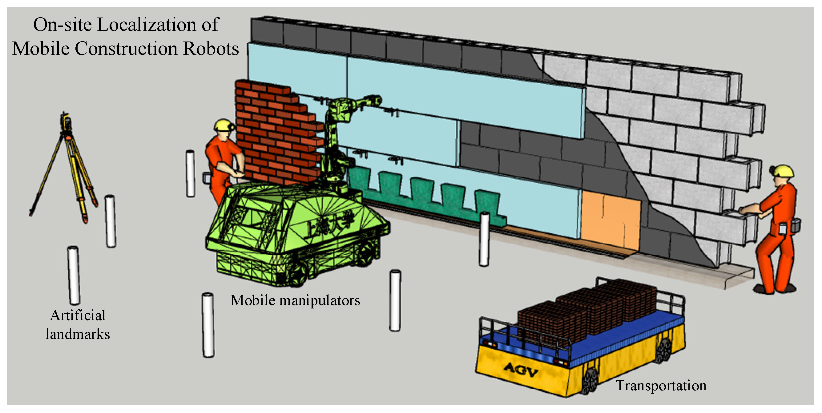
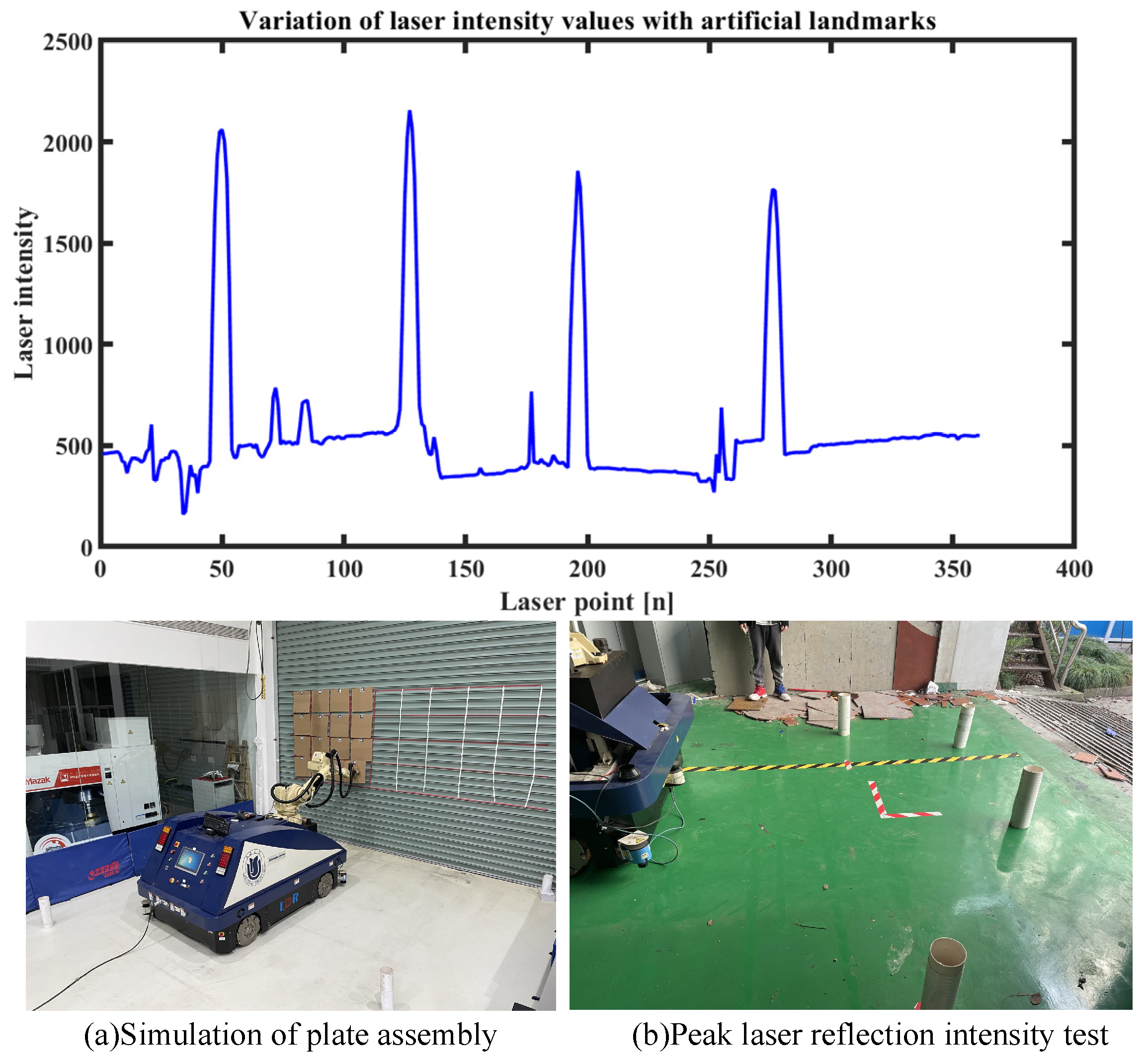
- An artificial landmark detection approach based on laser reflection intensity is proposed, and a trilateral localization algorithm is developed using the detection and identification results.
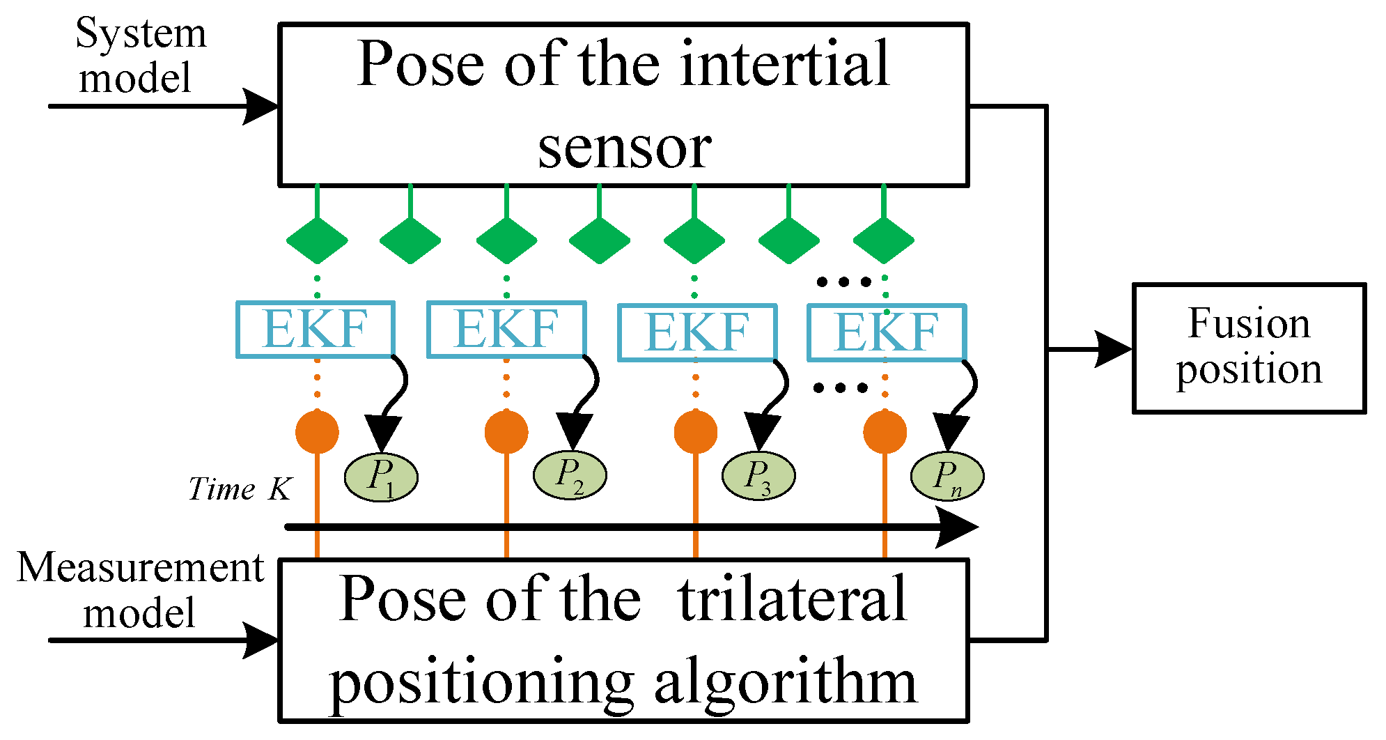
- The EKF-based multi-sensor fusion technique is adopted to achieve the integration of trilateral localization results and inertial sensor positioning results.
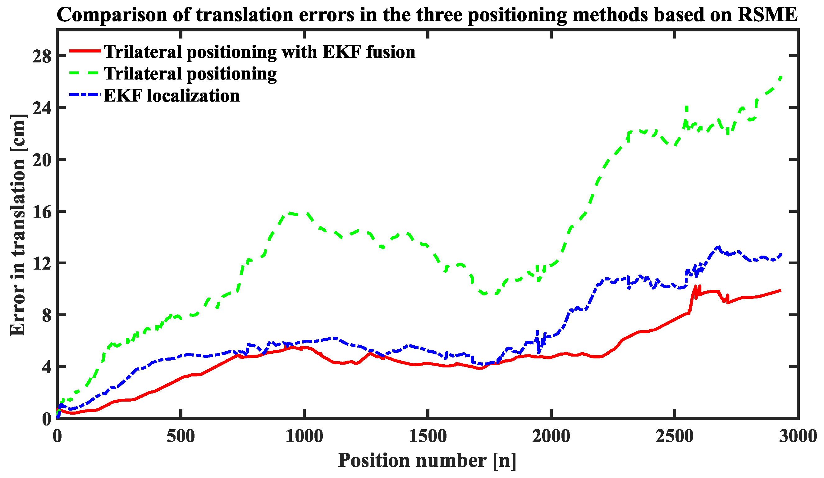
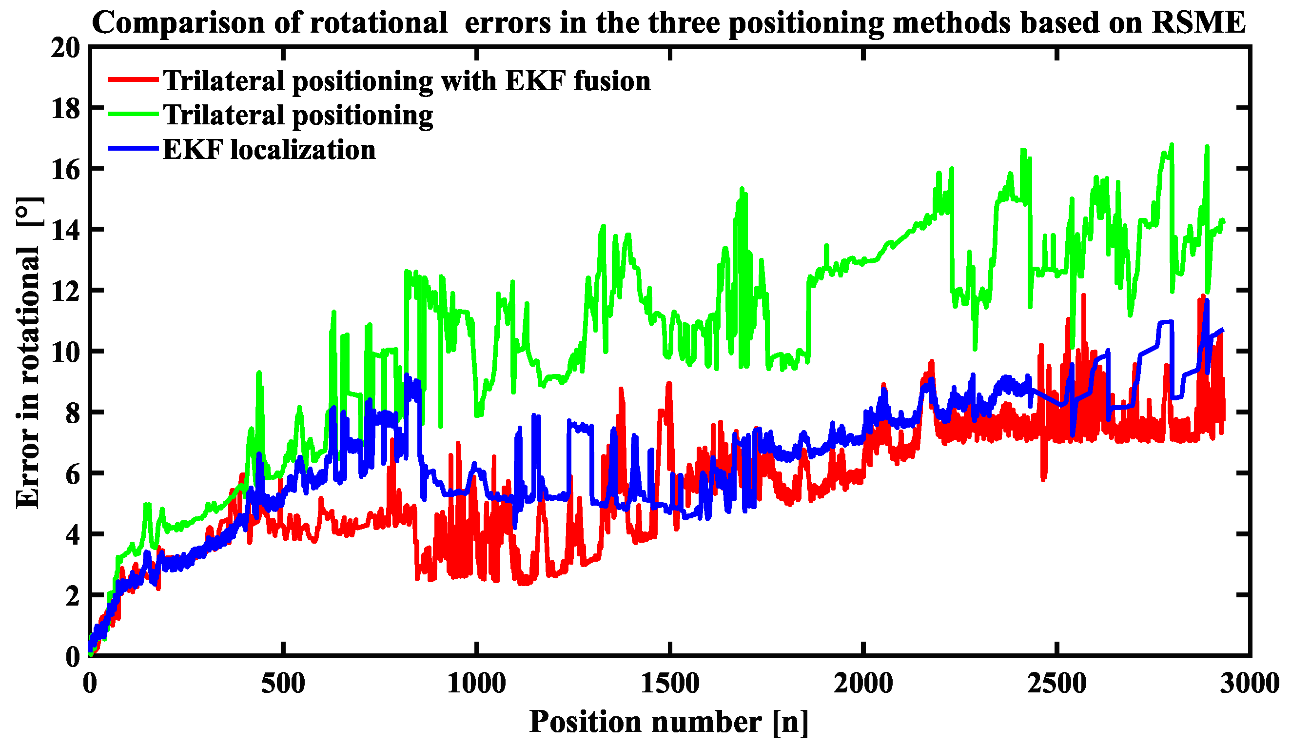
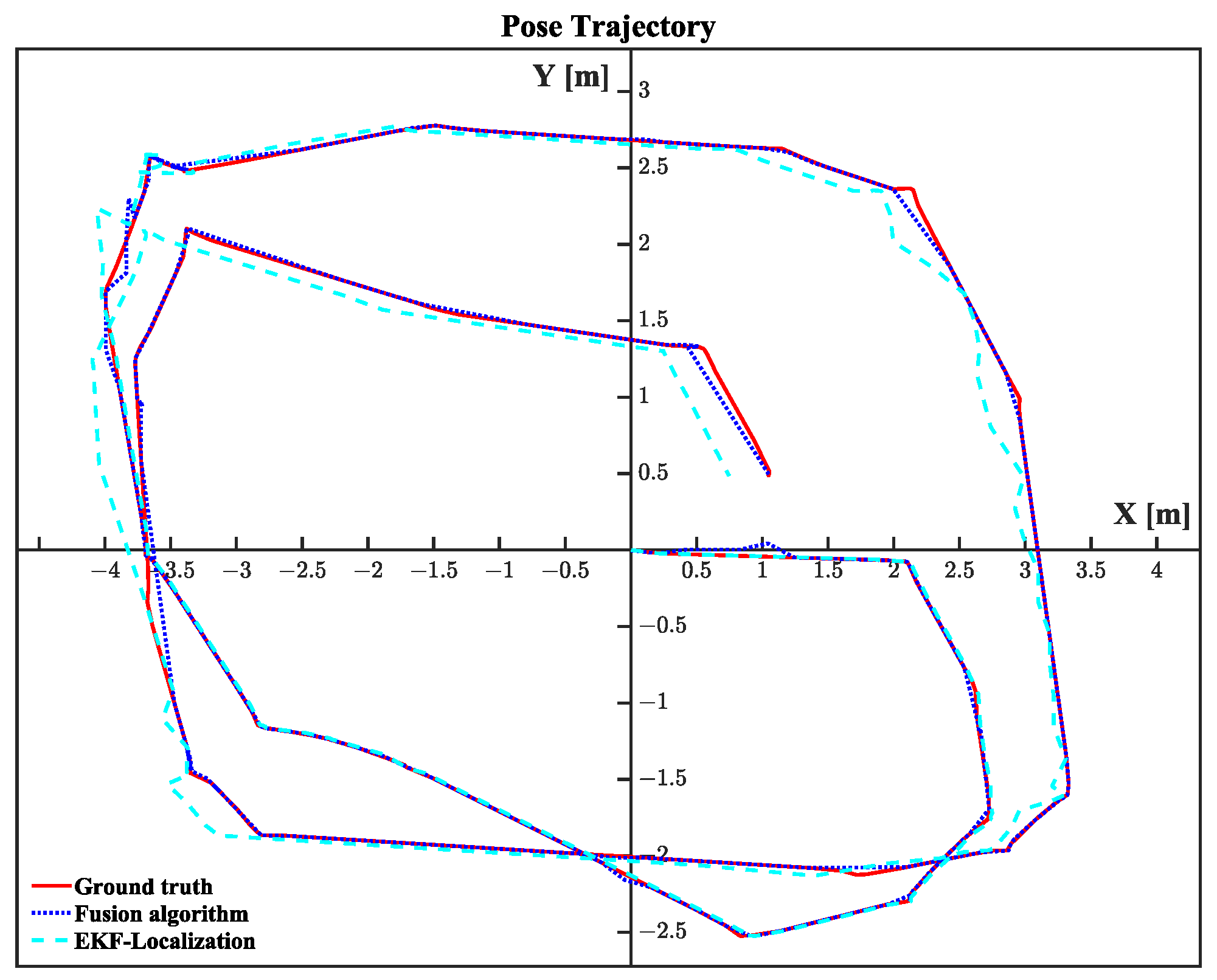
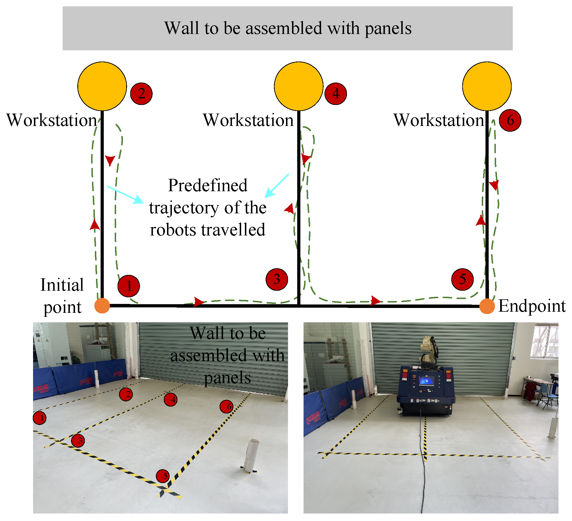
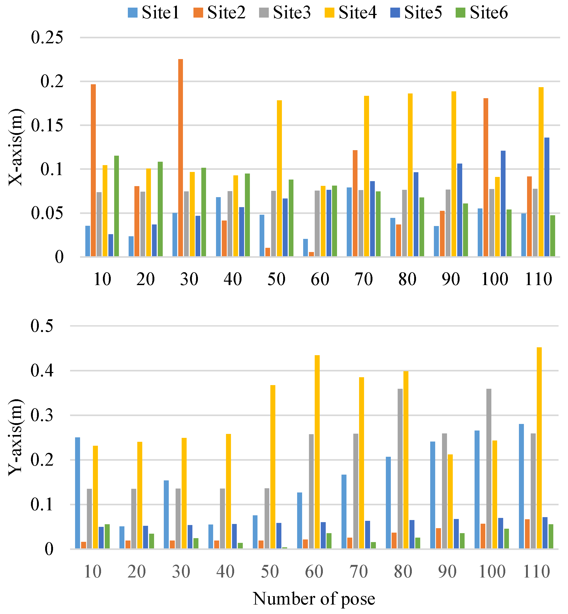
- The accuracy and practicality of the algorithm are verified in simulation and real environments, respectively. The experimental results demonstrate the usability of the algorithm.
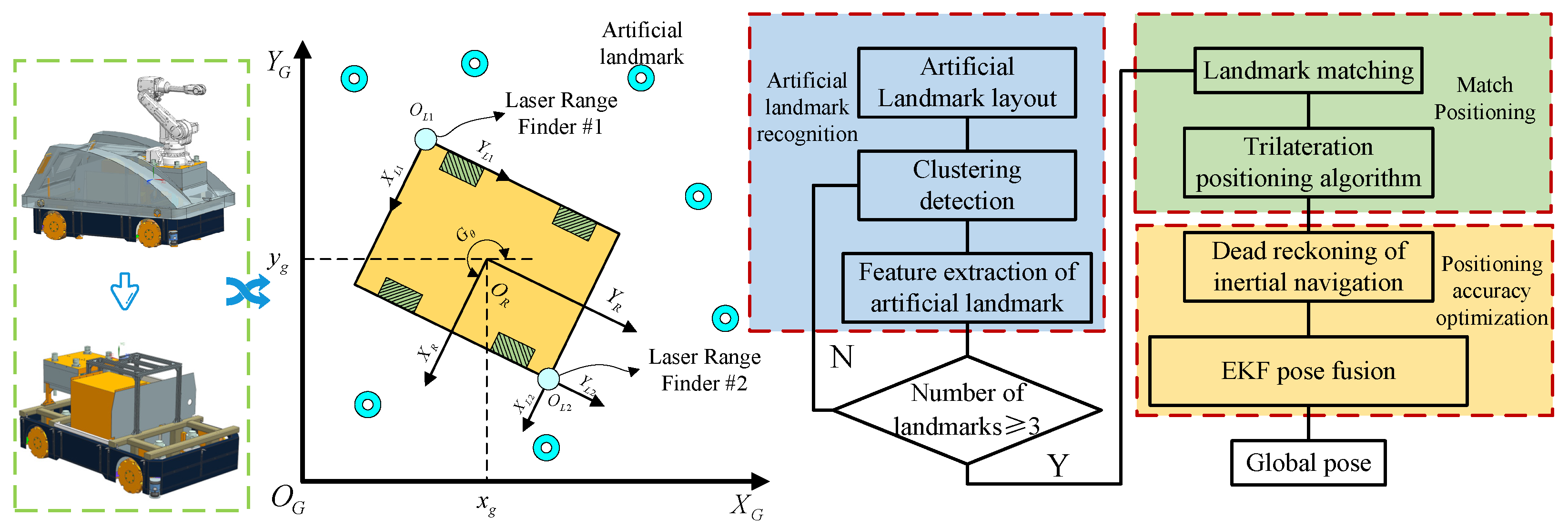
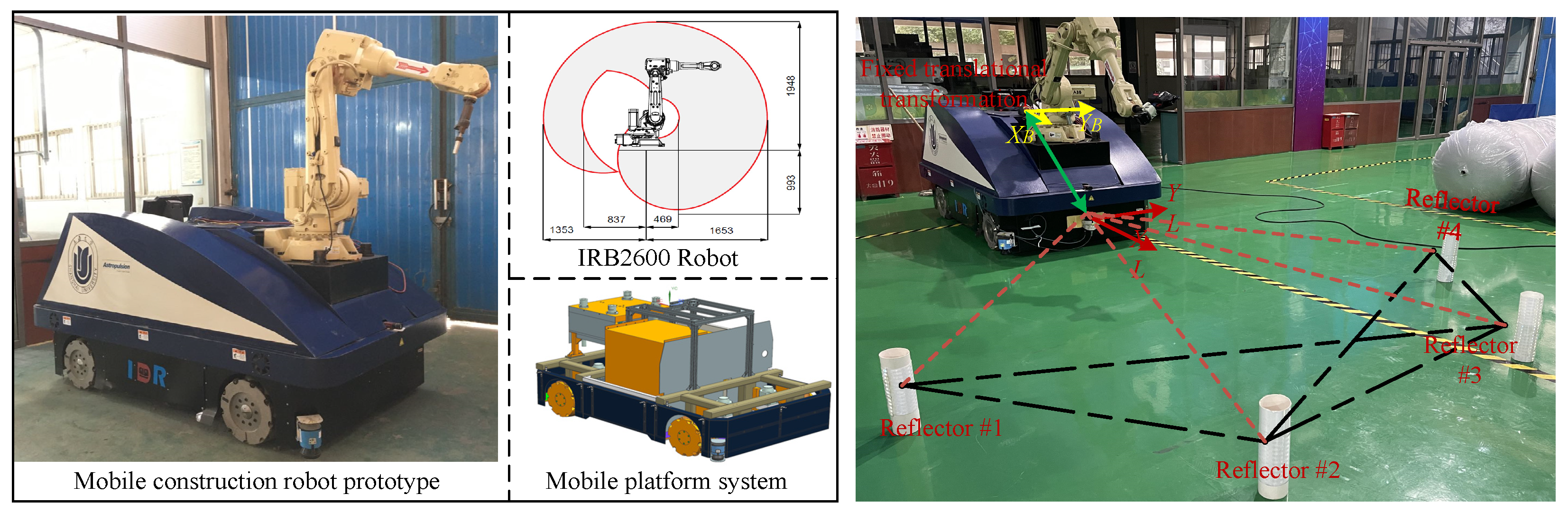
2. System Overview
3. Methodology
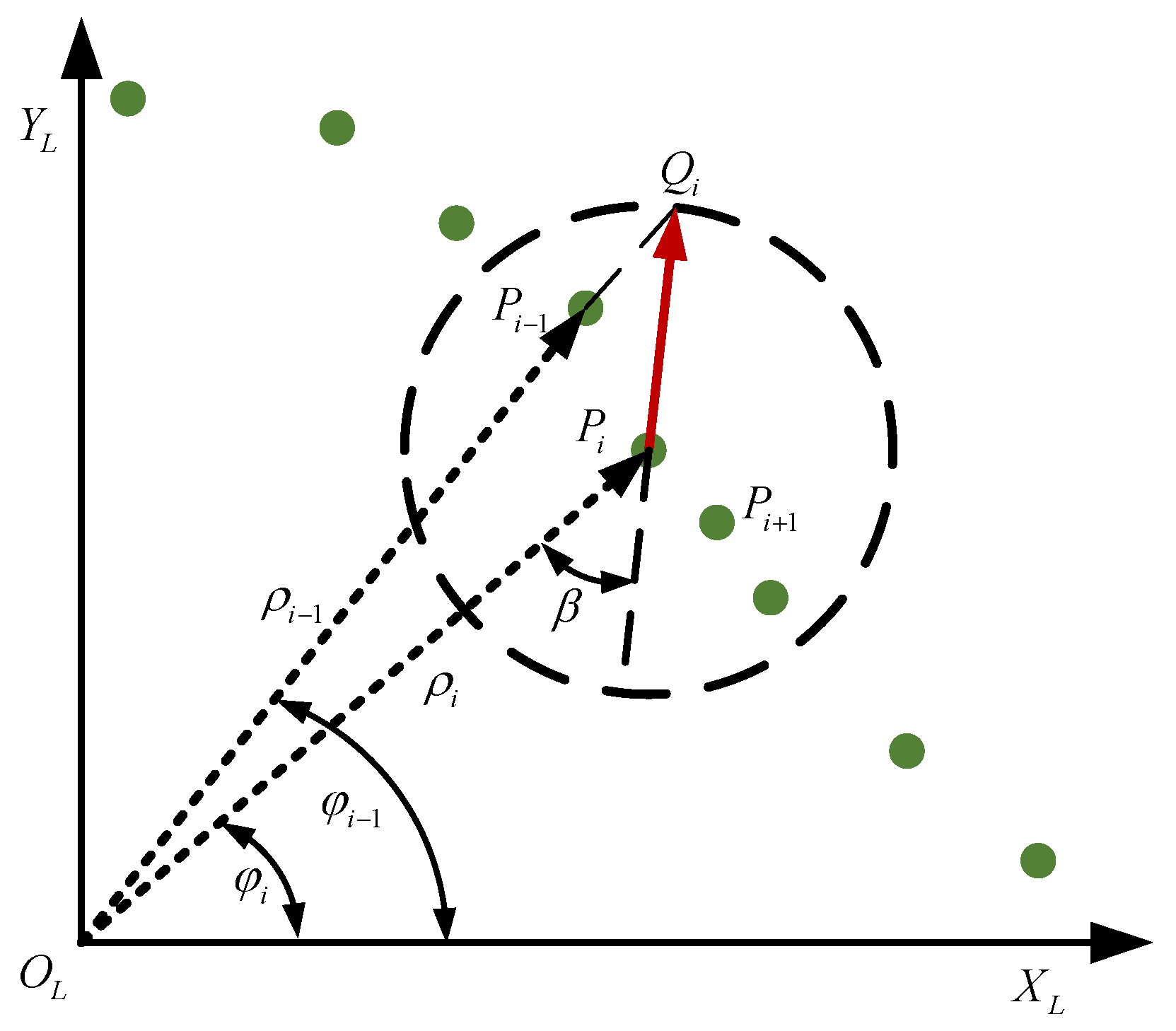
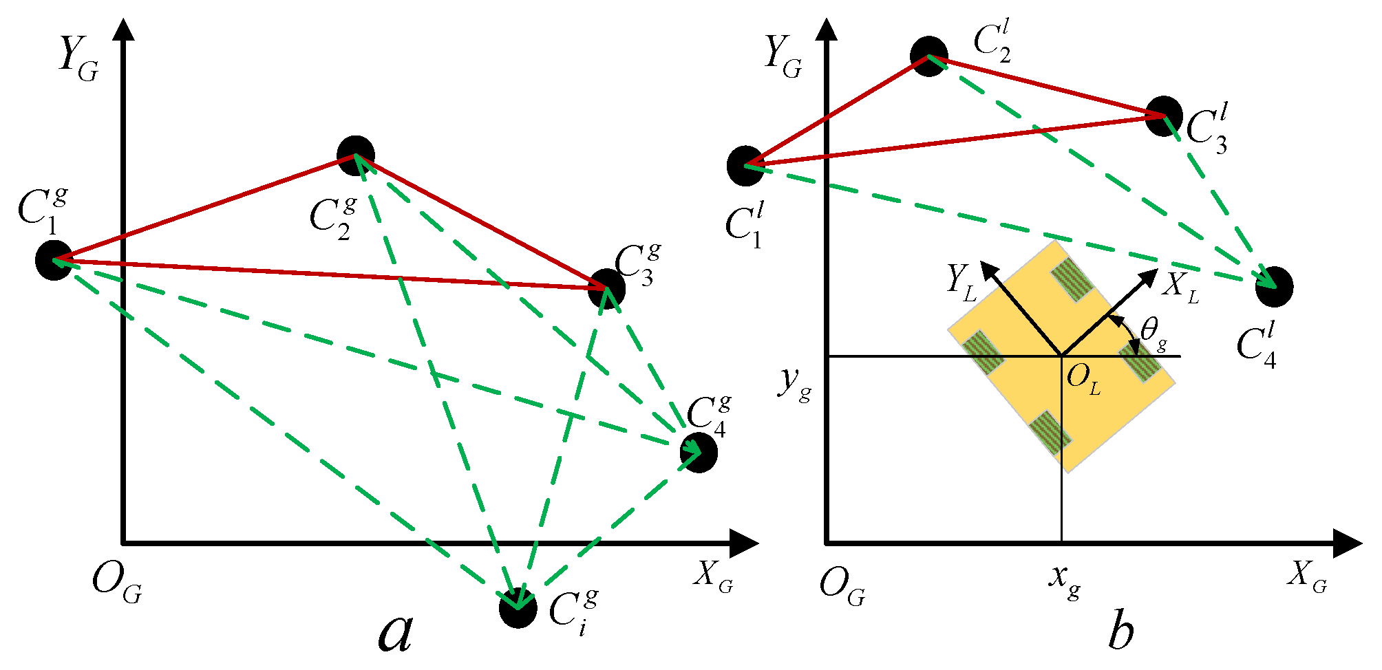
3.1. Identification and Extraction of Artificial Landmarks
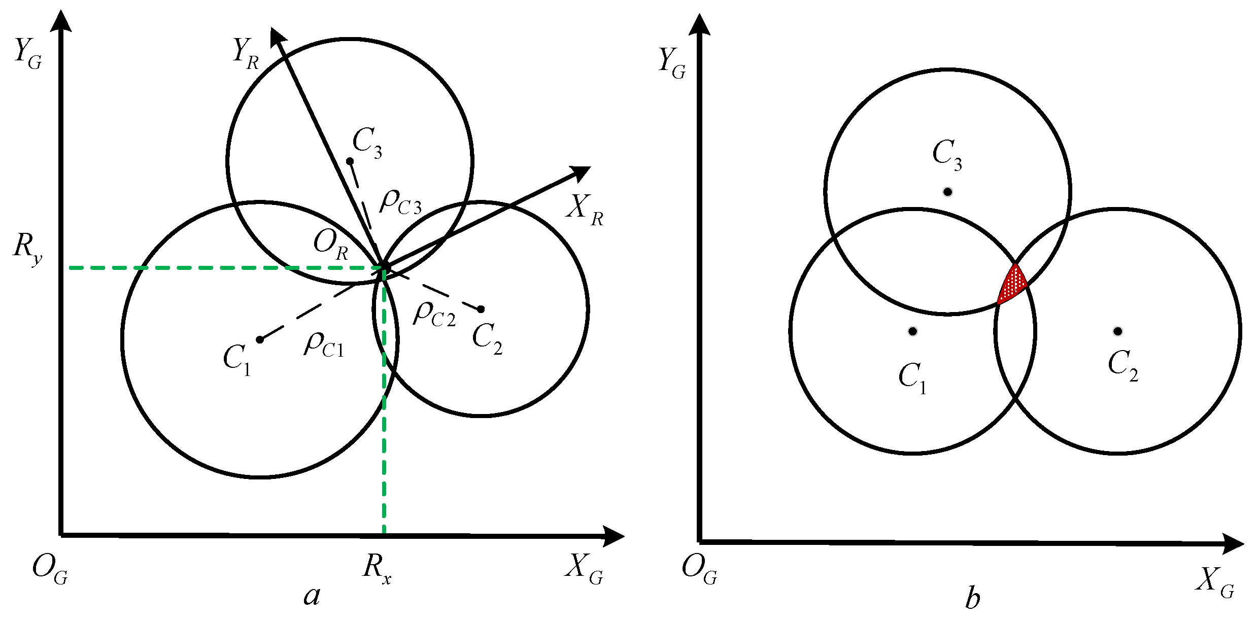
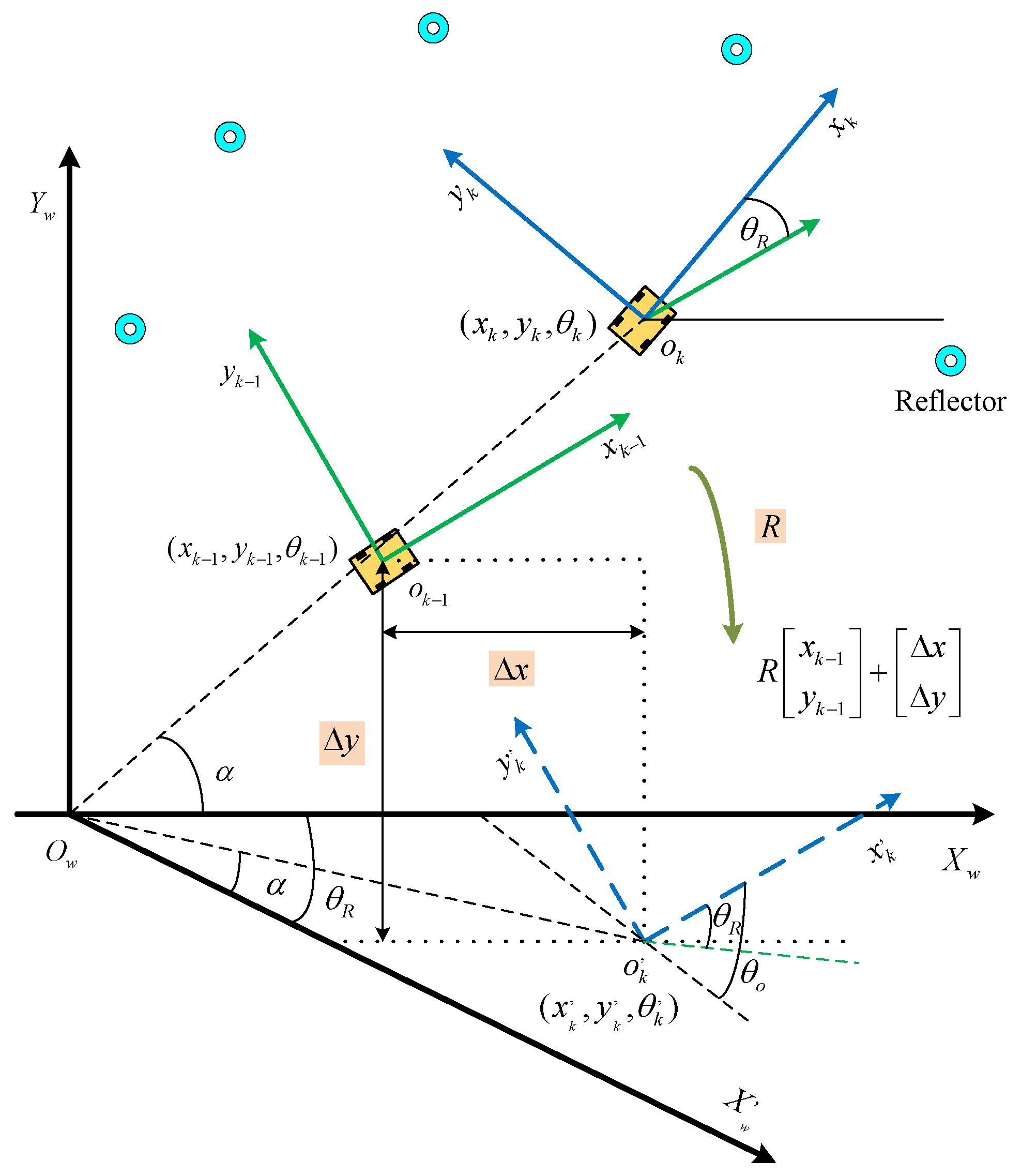
3.2. Trilateral Positioning for Mobile Construction Robot
| Algorithm 1: Trilateral localization using reflectors. |
 |
3.3. Positioning Accuracy Improvements Based on EKF
| Algorithm 2: Positioning accuracy improvements based on EKF. |
Input: Estimated robot pose at an initial time: , Noise variance in the moving model: , Noise variance in the measured model: Output: Optimal pose estimation: 1 Calculate the forward state variable at time k: 2 Calculate the prediction error covariance matrix: 3 Obtain the measured current pose value from trilateral positioning: 4 Calculate the Kalman gain matrix: 5 Update the state variable at time k: 6 Calculate the estimated error covariance: 7 Return |
4. Verification Experiments
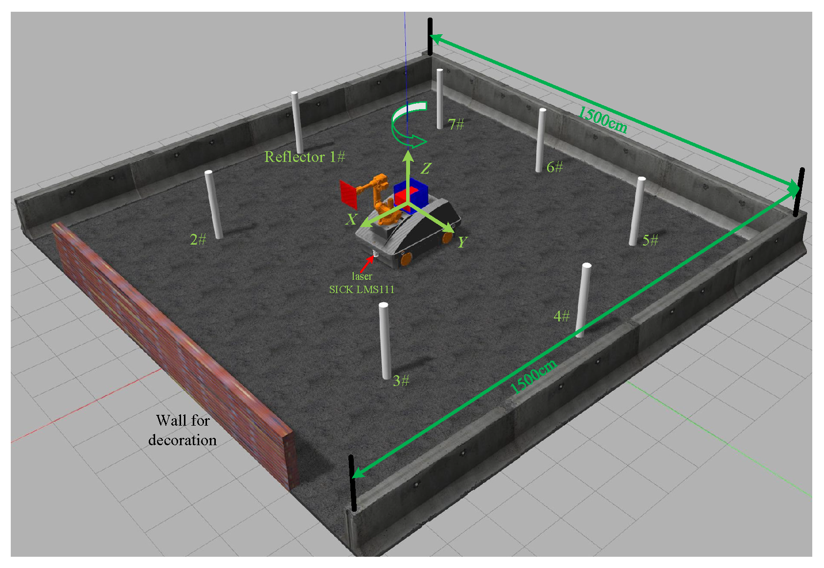
4.1. Initialization and Experimental Settings
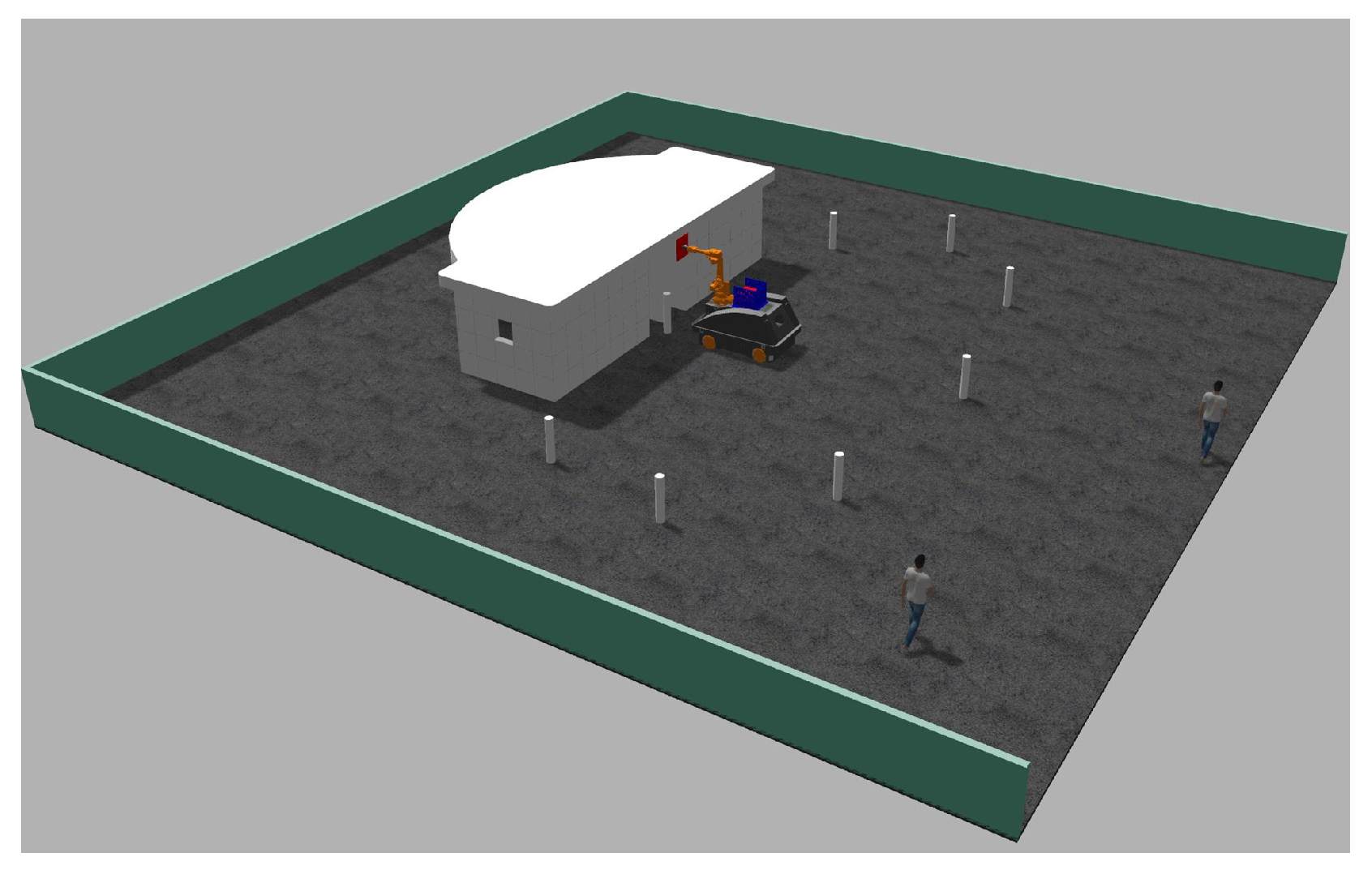
4.2. Validation with Gazebo
4.3. Testing in Physical Environments
5. Conclusions
Author Contributions
Funding
Data Availability Statement
Conflicts of Interest
References
- Debrah, C.; Chan, A.P.; Darko, A. Artificial intelligence in green building. Autom. Constr. 2022, 137, 104192. [Google Scholar] [CrossRef]
- de Soto, B.G.; Agustí-Juan, I.; Hunhevicz, J.; Joss, S.; Graser, K.; Habert, G.; Adey, B.T. Productivity of digital fabrication in construction: Cost and time analysis of a robotically built wall. Autom. Constr. 2018, 92, 297–311. [Google Scholar] [CrossRef]
- Petersen, K.H.; Napp, N.; Stuart-Smith, R.; Rus, D.; Kovac, M. A review of collective robotic construction. Sci. Robot. 2019, 4, eaau8479. [Google Scholar] [CrossRef] [PubMed]
- Štibinger, P.; Broughton, G.; Majer, F.; Rozsypálek, Z.; Wang, A.; Jindal, K.; Zhou, A.; Thakur, D.; Loianno, G.; Krajník, T.; et al. Mobile manipulator for autonomous localization, grasping and precise placement of construction material in a semi-structured environment. IEEE Robot. Autom. Lett. 2021, 6, 2595–2602. [Google Scholar] [CrossRef]
- Dörfler, K.; Dielemans, G.; Lachmayer, L.; Recker, T.; Raatz, A.; Lowke, D.; Gerke, M. Additive Manufacturing using mobile robots: Opportunities and challenges for building construction. Cem. Concr. Res. 2022, 158, 106772. [Google Scholar] [CrossRef]
- Gawel, A.; Blum, H.; Pankert, J.; Krämer, K.; Bartolomei, L.; Ercan, S.; Farshidian, F.; Chli, M.; Gramazio, F.; Siegwart, R.; et al. A fully-integrated sensing and control system for high-accuracy mobile robotic building construction. In Proceedings of the IEEE/RSJ International Conference on Intelligent Robots and Systems (IROS), Macau, China, 3–8 November 2019; pp. 2300–2307. [Google Scholar] [CrossRef]
- Melenbrink, N.; Werfel, J.; Menges, A. On-site autonomous construction robots: Towards unsupervised building. Autom. Constr. 2020, 119, 103312. [Google Scholar] [CrossRef]
- Gharbia, M.; Chang-Richards, A.; Lu, Y.; Zhong, R.Y.; Li, H. Robotic technologies for on-site building construction: A systematic review. J. Build. Eng. 2020, 32, 101584. [Google Scholar] [CrossRef]
- Sandy, T.; Giftthaler, M.; Dörfler, K.; Kohler, M.; Buchli, J. Autonomous repositioning and localization of an in situ fabricator. In Proceedings of the IEEE International Conference on Robotics and Automation (ICRA), Stockholm, Sweden, 16–21 May 2016; pp. 2852–2858. [Google Scholar] [CrossRef]
- Lussi, M.; Sandy, T.; Dörfler, K.; Hack, N.; Gramazio, F.; Kohler, M.; Buchli, J. Accurate and adaptive in situ fabrication of an undulated wall using an on-board visual sensing system. In Proceedings of the IEEE International Conference on Robotics and Automation (ICRA), Brisbane, QLD, Australia, 21–25 May 2018; pp. 3532–3539. [Google Scholar] [CrossRef]
- Hack, N.; Lauer, W.V. Mesh-mould: Robotically fabricated spatial meshes as reinforced concrete formwork. Archit. Des. 2014, 84, 44–53. [Google Scholar] [CrossRef]
- Yin, H.; Lin, Z.; Yeoh, J.K. Semantic localization on BIM-generated maps using a 3D LiDAR sensor. Autom. Constr. 2023, 146, 104641. [Google Scholar] [CrossRef]
- Xu, Z.; Guo, S.; Song, T.; Zeng, L. Robust localization of the mobile robot driven by LiDAR measurement and matching for ongoing scene. Appl. Sci. 2020, 10, 6152. [Google Scholar] [CrossRef]
- Ardiny, H.; Witwicki, S.; Mondada, F. Construction automation with autonomous mobile robots: A review. In Proceedings of the 3rd RSI International Conference on Robotics and Mechatronics (ICROM), Tehran, Iran, 7–9 October 2015; pp. 418–424. [Google Scholar] [CrossRef]
- Dörfler, K.; Hack, N.; Sandy, T.; Giftthaler, M.; Lussi, M.; Walzer, A.N.; Buchli, J.; Gramazio, F.; Kohler, M. Mobile robotic fabrication beyond factory conditions: Case study Mesh Mould wall of the DFAB HOUSE. Constr. Robot. 2019, 3, 53–67. [Google Scholar] [CrossRef]
- Giftthaler, M.; Sandy, T.; Dörfler, K.; Brooks, I.; Buckingham, M.; Rey, G.; Kohler, M.; Gramazio, F.; Buchli, J. Mobile robotic fabrication at 1: 1 scale: The In situ Fabricator: System, experiences and current developments. Constr. Robot. 2017, 1, 3–14. [Google Scholar] [CrossRef]
- Ercan, S.; Meier, S.; Gramazio, F.; Kohler, M. Automated localization of a mobile construction robot with an external measurement device. In Proceedings of the 36th International Symposium on Automation and Robotics in Construction (ISARC 2019), Banff, AB, Canada, 21–24 May 2019; pp. 929–936. [Google Scholar] [CrossRef]
- Cadena, C.; Carlone, L.; Carrillo, H.; Latif, Y.; Scaramuzza, D.; Neira, J.; Reid, I.; Leonard, J.J. Past, present, and future of simultaneous localization and mapping: Toward the robust-perception age. IEEE Trans. Robot. 2016, 32, 1309–1332. [Google Scholar] [CrossRef]
- Kim, P.; Chen, J.; Cho, Y.K. SLAM-driven robotic mapping and registration of 3D point clouds. Autom. Constr. 2018, 89, 38–48. [Google Scholar] [CrossRef]
- Basiri, M.; Gonçalves, J.; Rosa, J.; Vale, A.; Lima, P. An autonomous mobile manipulator to build outdoor structures consisting of heterogeneous brick patterns. SN Appl. Sci. 2021, 3, 558. [Google Scholar] [CrossRef]
- Lakhal, O.; Chettibi, T.; Belarouci, A.; Dherbomez, G.; Merzouki, R. Robotized additive manufacturing of funicular architectural geometries based on building materials. IEEE/ASME Trans. Mechatron. 2020, 25, 2387–2397. [Google Scholar] [CrossRef]
- Yan, R.J.; Kayacan, E.; Chen, I.M.; Tiong, L.K.; Wu, J. QuicaBot: Quality inspection and assessment robot. IEEE Trans. Autom. Sci. Eng. 2018, 16, 506–517. [Google Scholar] [CrossRef]
- Zhang, X.; Li, M.; Lim, J.H.; Weng, Y.; Tay, Y.W.D.; Pham, H.; Pham, Q.C. Large-scale 3D printing by a team of mobile robots. Autom. Constr. 2018, 95, 98–106. [Google Scholar] [CrossRef]
- Zhang, L.; Zapata, R.; Lepinay, P. Self-adaptive Monte Carlo localization for mobile robots using range finders. Robotica 2012, 30, 229–244. [Google Scholar] [CrossRef]
- Tiryaki, M.E.; Zhang, X.; Pham, Q.C. Printing-while-moving: A new paradigm for large-scale robotic 3D Printing. In Proceedings of the IEEE/RSJ International Conference on Intelligent Robots and Systems (IROS), Macau, China, 3–8 November 2019; pp. 2286–2291. [Google Scholar] [CrossRef]
- Lázaro, M.T.; Capobianco, R.; Grisetti, G. Efficient long-term mapping in dynamic environments. In Proceedings of the IEEE/RSJ International Conference on Intelligent Robots and Systems (IROS), Madrid, Spain, 1–5 October 2018; pp. 153–160. [Google Scholar] [CrossRef]
- Moura, M.S.; Rizzo, C.; Serrano, D. Bim-based localization and mapping for mobile robots in construction. In Proceedings of the IEEE International Conference on Autonomous Robot Systems and Competitions (ICARSC), Santa Maria da Feira, Portugal, 28–29 April 2021; pp. 12–18. [Google Scholar] [CrossRef]
- Kim, K.; Peavy, M. BIM-based semantic building world modeling for robot task planning and execution in built environments. Autom. Constr. 2022, 138, 104247. [Google Scholar] [CrossRef]
- Zhao, X.; Cheah, C.C. BIM-based indoor mobile robot initialization for construction automation using object detection. Autom. Constr. 2023, 146, 104647. [Google Scholar] [CrossRef]
- Xie, D.J.; Zeng, L.D.; Xu, Z.; Guo, S.; Cui, G.H.; Song, T. Base position planning of mobile manipulators for assembly tasks in construction environments. Adv. Manuf. 2023, 11, 93–110. [Google Scholar] [CrossRef]
- Campbell, S.; O’Mahony, N.; Carvalho, A.; Krpalkova, L.; Riordan, D.; Walsh, J. Where am I? Localization techniques for mobile robots a review. In Proceedings of the 6th International Conference on Mechatronics and Robotics Engineering (ICMRE), Barcelona, Spain, 12–15 February 2020; pp. 43–47. [Google Scholar] [CrossRef]
- Feng, X.; Guo, S.; Li, X.; He, Y. Robust mobile robot localization by tracking natural landmarks. In Proceedings of the Artificial Intelligence and Computational Intelligence: International Conference, AICI 2009, Shanghai, China, 7–8 November 2009; Proceedings 1. Springer: Berlin/Heidelberg, Germany, 2009; pp. 278–287. [Google Scholar] [CrossRef]
- Zhou, Y. An efficient least-squares trilateration algorithm for mobile robot localization. In Proceedings of the IEEE/RSJ International Conference on Intelligent Robots and Systems, St. Louis, MO, USA, 10–15 October 2009; pp. 3474–3479. [Google Scholar] [CrossRef]
- Xu, H.; Ding, Y.; Wang, R.; Shen, W.; Li, P. A novel radio frequency identification three-dimensional indoor positioning system based on trilateral positioning algorithm. J. Algorithms Comput. Technol. 2016, 10, 158–168. [Google Scholar] [CrossRef]
- Zheng, S.; Li, Z.; Liu, Y.; Zhang, H.; Zou, X. An optimization-based UWB-IMU fusion framework for UGV. IEEE Sens. J. 2022, 22, 4369–4377. [Google Scholar] [CrossRef]
- Censi, A.; Franchi, A.; Marchionni, L.; Oriolo, G. Simultaneous calibration of odometry and sensor parameters for mobile robots. IEEE Trans. Robot. 2013, 29, 475–492. [Google Scholar] [CrossRef]
- Li, C.; Wang, S.; Zhuang, Y.; Yan, F. Deep sensor fusion between 2D laser scanner and IMU for mobile robot localization. IEEE Sens. J. 2019, 21, 8501–8509. [Google Scholar] [CrossRef]
- Erdem, A.T.; Ercan, A.Ö. Fusing inertial sensor data in an extended Kalman filter for 3D camera tracking. IEEE Trans. Image Process. 2014, 24, 538–548. [Google Scholar] [CrossRef] [PubMed]
- Cui, Y.; Liu, S.; Yao, J.; Gu, C. Integrated positioning system of unmanned automatic vehicle in coal mines. IEEE Trans. Instrum. Meas. 2021, 70, 8503013. [Google Scholar] [CrossRef]
- Wang, J.; Alipouri, Y.; Huang, B. Dual neural extended Kalman filtering approach for multirate sensor data fusion. IEEE Trans. Instrum. Meas. 2020, 70, 6502109. [Google Scholar] [CrossRef]
- Teslić, L.; Škrjanc, I.; Klančar, G. EKF-based localization of a wheeled mobile robot in structured environments. J. Intell. Robot. Syst. 2011, 62, 187–203. [Google Scholar] [CrossRef]
- Zhu, J.; Kia, S.S. Cooperative localization under limited connectivity. IEEE Trans. Robot. 2019, 35, 1523–1530. [Google Scholar] [CrossRef]
- Yu, C.; Liu, Z.; Liu, X.J.; Xie, F.; Yang, Y.; Wei, Q.; Fei, Q. DS-SLAM: A semantic visual SLAM towards dynamic environments. In Proceedings of the IEEE/RSJ International Conference on Intelligent Robots and Systems (IROS), Madrid, Spain, 1–5 October 2018; pp. 1168–1174. [Google Scholar] [CrossRef]


| No. | Axis | 1# | 2# | 3# | 4# | 5# | 6# | 7# |
|---|---|---|---|---|---|---|---|---|
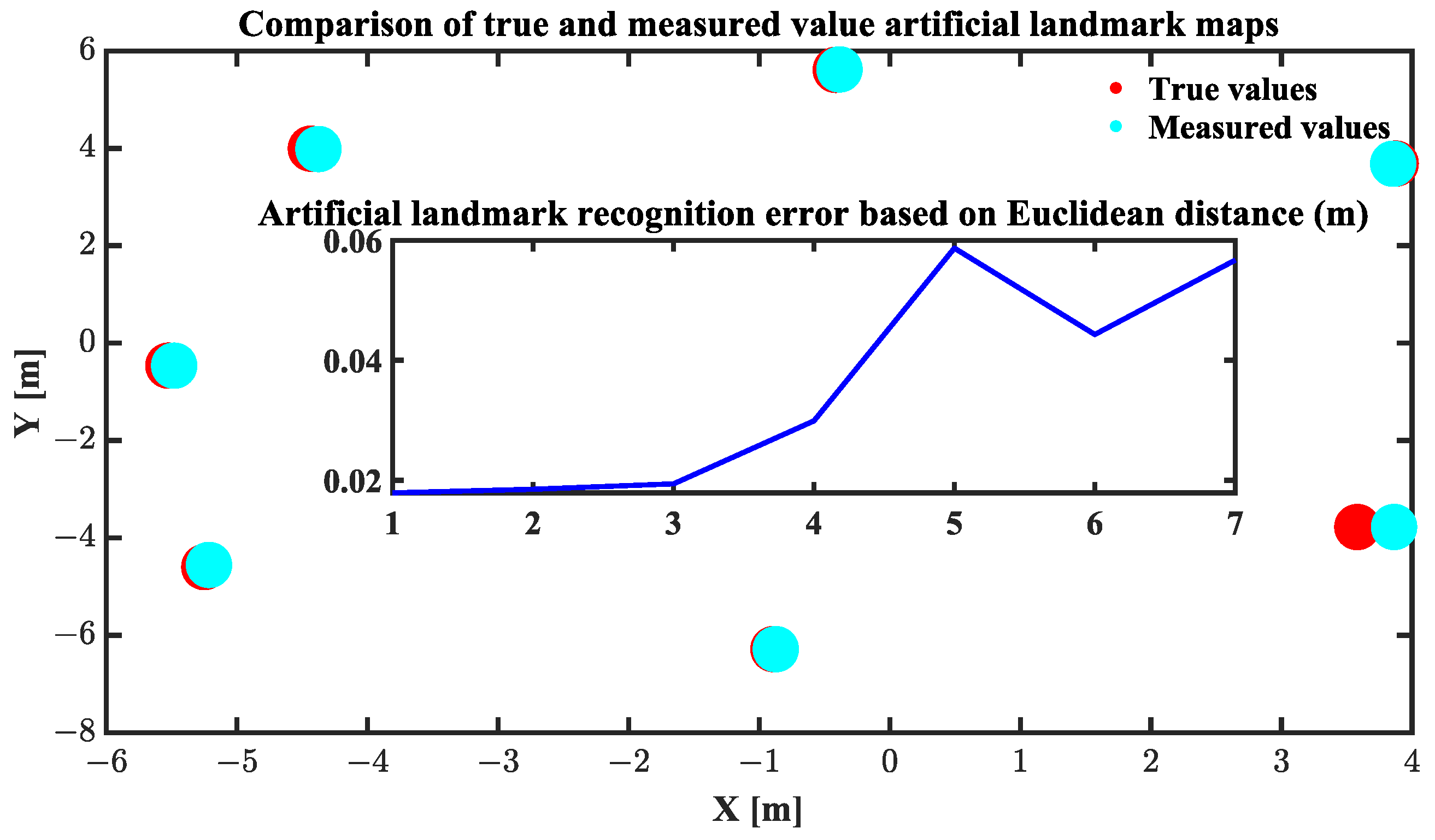
| True value | X-axis | −0.89 | 3.58 | 3.87 | −0.41 | −4.43 | −5.52 | −5.24 |
| Y-axis | −6.28 | −3.77 | 3.68 | 5.61 | 3.99 | −0.46 | −4.59 | |
| Measured values | X-axis | −0.87 | 3.86 | 3.85 | −0.38 | −4.37 | −5.48 | −5.21 |
| Y-axis | −6.28 | −3.77 | 3.68 | 5.61 | 3.98 | −0.46 | −4.55 | |
| Euclidean distance | \ | 0.02 | 0.02 | 0.02 | 0.03 | 0.06 | 0.04 | 0.05 |
| Site | Coordinate Axis | Site1 | Site2 | Site3 | Site4 | Site5 | Site6 |
|---|---|---|---|---|---|---|---|
| Ideal value (m) | X-axis | 0 | 3 | 0 | 3 | 0 | 3 |
| Y-axis | 0 | 0 | 1.2 | 1.2 | 2.4 | 2.4 | |
| Output value (m) | X-axis | 0.018 | 3.071 | −0.075 | 3.064 | 0.077 | 2.911 |
| Y-axis | 0.014 | 0.031 | 1.221 | 1.315 | 2.461 | 2.382 |
Disclaimer/Publisher’s Note: The statements, opinions and data contained in all publications are solely those of the individual author(s) and contributor(s) and not of MDPI and/or the editor(s). MDPI and/or the editor(s) disclaim responsibility for any injury to people or property resulting from any ideas, methods, instructions or products referred to in the content. |
© 2024 by the authors. Licensee MDPI, Basel, Switzerland. This article is an open access article distributed under the terms and conditions of the Creative Commons Attribution (CC BY) license (https://creativecommons.org/licenses/by/4.0/).
Share and Cite
Zeng, L.; Guo, S.; Zhu, M.; Duan, H.; Bai, J. An Improved Trilateral Localization Technique Fusing Extended Kalman Filter for Mobile Construction Robot. Buildings 2024, 14, 1026. https://doi.org/10.3390/buildings14041026
Zeng L, Guo S, Zhu M, Duan H, Bai J. An Improved Trilateral Localization Technique Fusing Extended Kalman Filter for Mobile Construction Robot. Buildings. 2024; 14(4):1026. https://doi.org/10.3390/buildings14041026
Chicago/Turabian StyleZeng, Lingdong, Shuai Guo, Mengmeng Zhu, Hao Duan, and Jie Bai. 2024. "An Improved Trilateral Localization Technique Fusing Extended Kalman Filter for Mobile Construction Robot" Buildings 14, no. 4: 1026. https://doi.org/10.3390/buildings14041026