Abstract
In the realm of architectural computing, this study explores the integration of parametric design with machine learning algorithms to advance the early design phase of tall buildings with outer diagrid systems. The success of such an endeavor relies heavily on a data-driven and artificial intelligence-enhanced workflow aimed at identifying key architectural and structural variables through a feature/response selection process within a supervised machine learning framework. By augmenting an initial dataset, which was notably limited, through four distinct techniques—namely Gaussian copula, conditional generative adversarial networks, Gaussian copula generative adversarial network, and variational autoencoder—this study demonstrates a methodical approach to data enhancement in architectural design. The results indicate a slight preference for the Gaussian copula method, attributed to its less complex hyperparameter tuning process. Evaluation through a random forest regressor revealed stable performance across various cross-validation techniques on synthetic data, although with an acceptable decrease in the coefficient of determination, from an original average score of 0.925 to an augmented score of 0.764. This investigation underscores the potential of artificial intelligence-powered computational tools to guide design decisions by pinpointing the variables with the most significant impact on relevant outputs, quantitatively assessing their influence through the accuracy of the employed machine learning methods.
1. Introduction
The relationship between architectural form and structural behavior is a complex interplay, often explored intuitively, during the early stages of building design, where not only the aesthetic tone is set but also significant implications for the material requirements and the overall construction costs are defined. The collaboration between architects and structural engineers is vital given the substantial implications of initial design decisions on material consumption and construction expenses [1,2,3,4]. However, finding harmony between architectural ambition and structural integrity can be a challenge: architects may visualize forms that resonate aesthetically, but these might not always align with the demands of structural efficiency; an ideal structure balances aesthetics with minimal deflection and optimal weight distribution.
In the early design stages, it is observed that architectural and structural preferences may diverge, as forms that are pleasing to architects might not align perfectly with structural requirements. Creative exploration through machine learning (ML), particularly for predicting structural performance, becomes possible nowadays as computational tools are offered to navigate this challenge. ML, especially, is seen as holding the promise of revolutionizing architectural design by predicting structural outcomes even before construction begins [5], thanks to the exploration of a number of possibilities far beyond human inspection. While the full potential of data-centric design has yet to be realized on a global scale, its possibilities are considered vast. Through parametric design, the exploration of diverse solutions for both form and efficiency is facilitated [1,2,3,4], and with these tools a multitude of design options can be explored by architects and engineers, optimizing both form and function.
It is worth noting again that the initial design choices are pivotal because, as they are made at the start, they can greatly influence the building’s final form, function, and financial implications, often leading to suboptimal solutions later [4]. Construction costs, which constitute approximately one-third of the budget, are heavily influenced by this phase [6,7,8].
The spotlight of this work is on tall structures, namely those incorporating outer diagrids [9,10]: the concept of transferring lateral load-bearing capabilities to façade elements (diagrids) not only minimizes the need for interior columns but also aligns with the necessity of ensuring structural efficiency. In other words, this design approach elegantly merges aesthetic design with structural efficacy. Various research studies have delved into the relationship between architectural form and structural behavior, suggesting that hyperboloid shapes may outperform cylindrical ones in certain scenarios; several investigations have also studied the effects of different upper and lower geometries on structural efficiency [11,12,13].
The growing trend of integrating ML, a key subset of artificial intelligence (AI), into building design, has led to innovative architectural prototypes and enhanced evaluations of structural efficiency [14,15,16,17]. For a broader understanding of the current status, opportunities, and challenges of AI and ML in the construction industry, refer to references [18,19,20]. As mentioned above, advanced tools like parametric design software [21] not only provide insights into structural performance but also empower specialists to generate a multitude of high-rise building geometries using computer-aided design, which can then be translated into structural codes capable of producing comprehensive data regarding the building response, even under complex loading conditions. Ultimately, AI tools based on ML [16] or deep learning (DL) [22] are adept at processing these outcomes and extracting insights into correlations between input and output variables efficiently, uncovering patterns beyond human capabilities. Previous studies have been conducted on this topic, focusing on finding the best solutions (or optimization perspectives [23,24,25]) and overarching decision-making models [26,27].
In the context of building structural design, the integration of ML and DL has been recognized as a recent development, but its growth is observed to be rapid. ML tools are employed to both estimate and evaluate structural performance. Data from numerical studies [28,29], experimental tests [30,31], and health monitoring of actual buildings over time [32,33] are often used in these evaluations. Significant interest has been shown in using ML to study how buildings might react during earthquakes, given ML’s proven capability to uncover hidden patterns in complex scenarios in fields like science and engineering [34]. For instance, a study from reference [35] involves subjecting a set of cross-laminated timber structures to horizontal acceleration records, with the resulting numerical simulations analyzed using classical ML regression algorithms to predict building drift ratios. In another study [36], researchers employed ML to distinguish physical from non-physical modes in the modal analysis of a 195-m-tall building. This approach revealed the first five modes and their damping ratios, highlighting their stochastic distribution. In ref. [37], the time history nonlinear responses of four case studies (all reinforced concrete structures) under seismic load are obtained through a DL approach exploiting a purely data-driven approach, showing good results for lower floors and possibly slightly less good for higher floors. The same research group also showed [38] that a multi-head attention mechanism can benefit from physical structural information to obtain the time histories of thousands of nodes in a structure in real time under seismic action. Particular attention should be placed on the inter-story drift when assessing the vulnerability of steel structures, see, e.g., [39].
A different approach is considered in this study: the emphasis is shifted to offering assistance to designers in the early design phase, where they can integrate human-guided architectural preferences. The ML process aims here to categorize buildings into viable choices that harmonize form and structural efficiency [40]. Feature selection (FS) plays a pivotal role in guiding architects and engineers toward choices that best merge aesthetic and structural considerations in the ML process, as it can identify the most influential design aspects. FS is actually a crucial step in data analysis and ML since it aims to extract the most relevant and informative attributes from a given dataset. By focusing on a chosen group of essential features, benefits such as reduced dimensionality, better model performance, and enhanced interpretability can be achieved [41,42]. Two main approaches dominate FS: the filter method and the sequential feature selection method. A filter method efficiently ranks attributes purely based on their statistical significance, while a sequential method, similar to a wrapper approach, evaluates a feature subset performance using a specific learning algorithm. Both methods aim to boost model precision and clarity while efficiently using computational resources, and they are discussed in this study in the specific context of the early design phase of tall buildings with outer diagrids. In our previous work [43], we already provided the results related to the filter method with a specific metric, the Pearson correlation coefficient, while here we show the alternative Spearman’s rank.
Given the complexity of building designs, especially in intricate structures, datasets available for machine learning might be limited. In such scenarios as the one that is considered in this work, data augmentation (DA) is indispensable. This process involves the expansion of dataset size when existing samples are found to be insufficient, by creating additional synthetic data points that enhance the learning capabilities of algorithms. This is especially vital for models like neural networks (NNs), which excel with large datasets. Moreover, it proves advantageous for algorithms characterized by volatile learning processes and outcomes contingent upon data samples, thus contributing to improved model performance and generalization. By generating novel synthetic data points, DA is established as a potent tool in tackling challenges arising from limited training data, bolstering the resilience and efficacy of machine learning models [44,45]. While in our previous work [43], we only showed the results for the Gaussian copula, in the present paper several alternative DA algorithms are instead comparatively evaluated.
2. Workflow
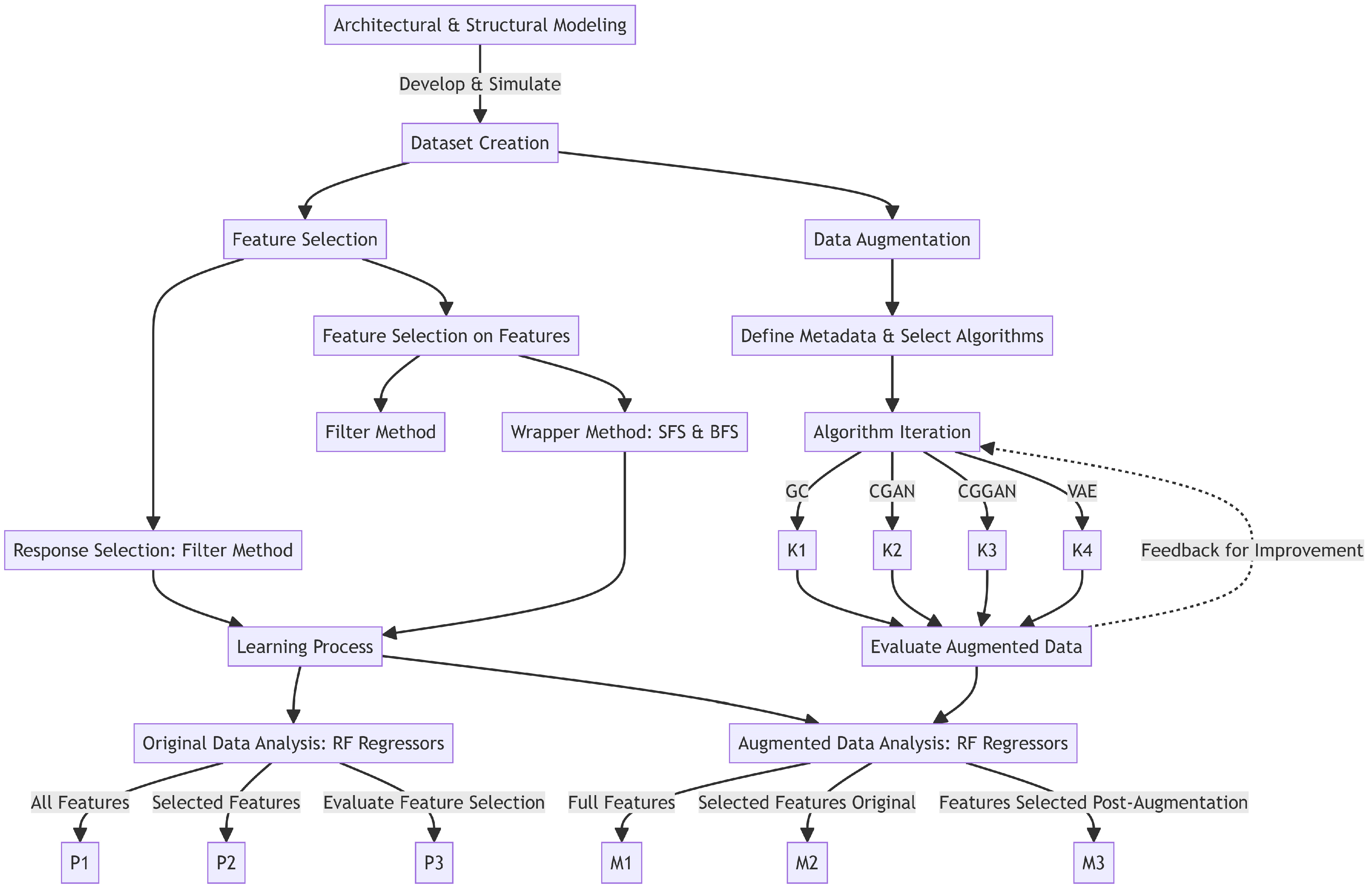
After the dataset has been built, see Section 3, the fundamental stages proposed in this work can be streamlined as follows and depicted in the flowchart shown in Figure 1. The flowchart includes detailed steps that will be described in the following Section 3, Section 4 and Section 5.
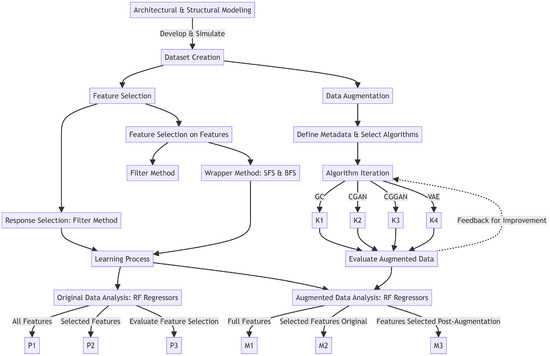
Figure 1.
Flowchart of the proposed procedure.
- Feature and response identification using various FS methods. During this step, essential features and responses are identified by using a range of feature selection (FS) techniques. The most relevant attributes from the dataset are extracted, ensuring alignment with the main goals of the study.
- Generating synthetic data and evaluating its quality with advanced AI algorithms. New synthetic data are created using advanced data augmentation (DA) algorithms. After generation, the accuracy and reliability of this augmented data are evaluated against the set standards of the research.
- Understanding the connection between architectural factors and structural reactions through AI-driven regression analysis. Once the prior steps are completed, regression techniques are adopted to explore the complex link between architectural factors and structural responses. The insights gained from the initial FS and DA stages are used to guide a detailed regression analysis. This step realizes an empirical framework that captures the intricate relationships existing between architectural elements and structural behaviors.
3. Dataset Construction
3.1. Architectural and Structural Modelling
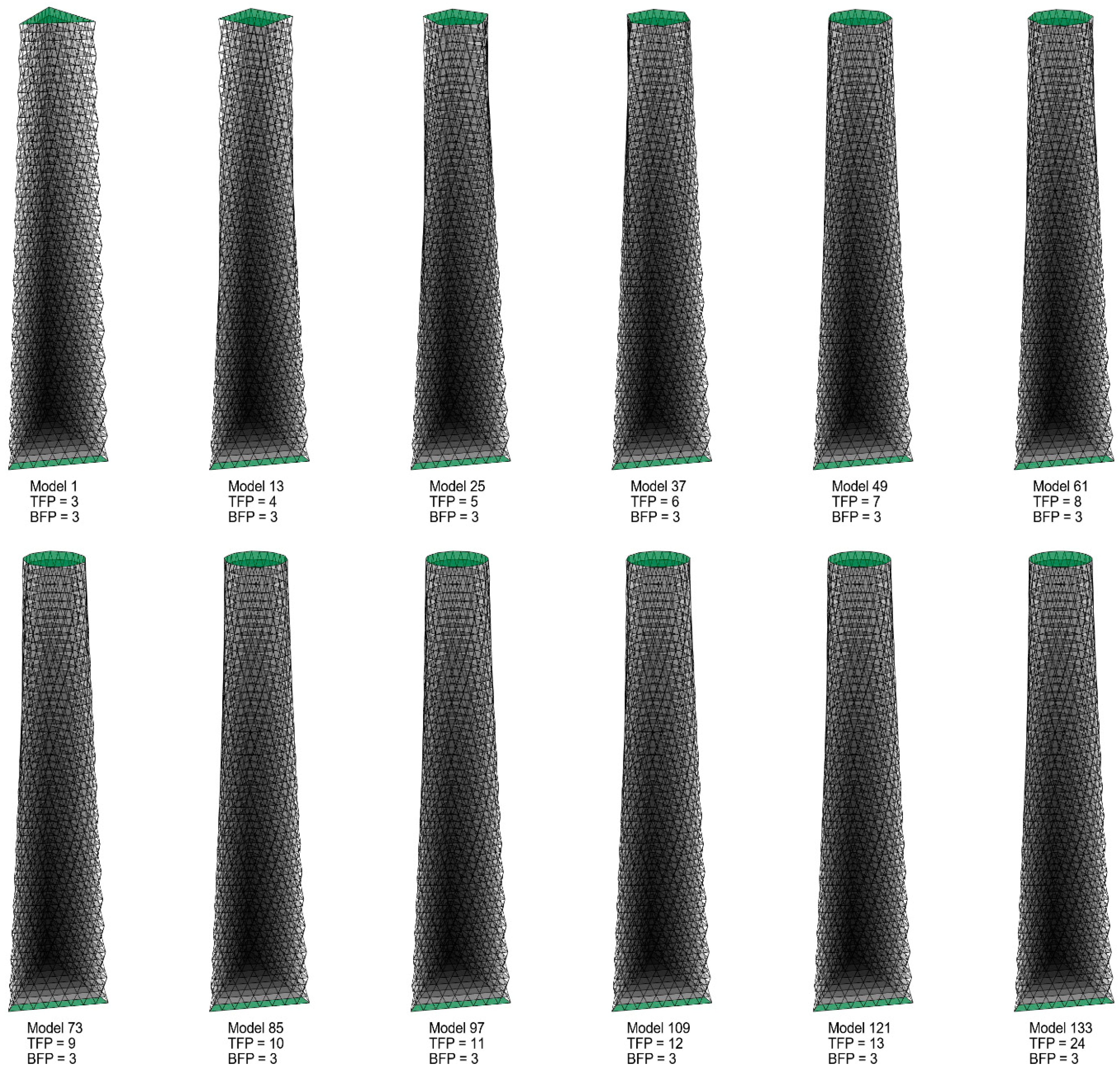
The dataset focuses on the structural results of a group of tall buildings under seismic (modeled as statically equivalent) loading. In particular, the dataset arises from merging different designs for the top and bottom floor plans of the tall buildings, see Figure 2. Additionally, within the Supplementary Materials of the research paper, there is an illustration encompassing all 144 models of tall buildings. These configurations include various polygonal shapes, from triangles (three sides) to 24-sided polygons adopted for the top and bottom floors of the buildings. As a result, a total of 144 distinct tall building models with outer diagrids are created in a design environment using the GrasshopperTM (Build 1.0.0007) and RhinocerosTM (Version 7 SR34) software. In this study, the Karamba3D plugin played a crucial role in the structural analysis of our models. Specifically, it was utilized to apply vertical static loads (self-weight, dead loads, and live loads on the floors) as well as lateral seismic loads, which were defined using the statically equivalent method. However, a detailed description of the dynamic effects is beyond the scope of this work, and therefore, the first mode was assumed to be dominant for a cantilevered structure and used to estimate the static equivalent forces in accordance with the guidelines provided in Eurocode 8. The integration of Karamba3D allowed for an efficient simulation of the structural behavior under these loads, enabling the evaluation of the diagrid system’s performance across all modeled buildings. Further details on the simulation procedure and parameters used in Karamba3D are elaborated in reference [40].
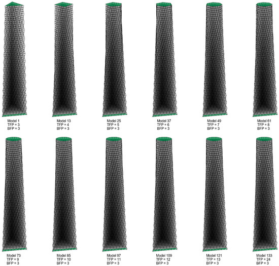
Figure 2.
A total of 12 samples out of 144 models, with the top floor plan (TFP) and bottom floor plan (BFP) evidenced in green color. The featured models showcase a 3-sided polygon as the BFP, with TFP ranging from 3-sided to 24-sided polygons.
This study examines the different outputs of the structural analysis, including but not limited to the displacement of the top story and the structural utilization. At the same time, the input data includes various architectural entities, such as the design of the top and bottom floor plans and the building’s height. Further insights about the structural analysis initial settings can be found in ref. [40].
3.2. Dataset Overview: Features and Responses
As noted previously, the dataset is divided into two main parts: building geometric parameters, which act as inputs, and structural responses, which are the outputs. Within the framework of the ML paradigm, these inputs are termed features, while the outputs are known as responses. The spectrum of geometric properties characterizing the building models primarily comprises architectural parameters, such as the geometries of the top and bottom plans, the building’s height, and total gross area (TGA). Moreover, several features hold relevance within the context of the structural modeling domain, e.g., the degree of diagrid inclination at the upper and lower extremities of the building, the overall mass (weight), and the position of the center of gravity.
In the overview of our dataset, which is divided into input features and output responses, it is essential to note the statistical characteristics that develop our analysis. The dataset encompasses a range of architectural and structural parameters, with each feature and response analyzed for minimum, maximum, mean values, and standard deviation. This statistical assessment, integral for understanding the variability and distribution within our dataset, ensures robustness and validity in our findings. For instance, the input feature of the total gross area ranges from 69,524.2218 to 70,629.0727 m2, with a mean value of 70,242.6778 m2 and a standard deviation of 157.4655 m2, reflecting the dataset’s diversity in building sizes. Similarly, the output response of the displacement of the top story exhibits a minimum of 0.8685 m, a maximum of 1.1419 m, a mean of 0.9316 m, and a standard deviation of 0.0510 m, indicating the varied structural behavior across our building models. These statistical insights are crucial for our subsequent machine learning processes and for validating the effectiveness of the data augmentation techniques applied.
On the other hand, the responses derive from numerical simulations illustrating how the buildings behave. These responses encompass important factors, including but not confined to the displacement of the top story, the maximal utilization ratio spanning all structural members of a given model, the expected design weight (EDW) (comprising the summation of the products of each member’s utilization and its weight) [40], as well as their integrated manifestations.
More specifically, the comprehensive list of the 13 features includes (see Table 1, first column): the number of the top plan sides; the number of the bottom plan sides; the total gross area; the building height; the building aspect ratio (AR); the diagrid angle (in degrees) at the top; the diagrid angle at the bottom; the average of the diagrid angle; the total façade area; the total amount of diagrids; the total length of the diagrid area; the total mass; the height of the center of gravity.

Table 1.
Spearman’s correlation coefficient for all 13 features and the 5 selected responses.
The full list of the 13 responses includes, instead (see also Figure 3, bottom line of the heat map): the displacement of the top story; the maximum utilization in compression; the maximum utilization in tension; the maximum normal force in compression; the maximum normal force in tension; the absolute value of the maximum normal force; the EDW; the elastic energy; the ratio displacement/total mass; the ratio displacement/EDW; the ratio EDW/AR; the ratio EDW/TGA; the ratio total mass/TGA.

Figure 3.
Response selection: heat map of Spearman’s rank correlation. Dark red tones represent positive correlations, dark blue shades indicate inverse correlations, and light gradations suggest minimal correlation levels.
4. Dataset Management
As mentioned above, identifying the most important features and responses is an essential step in view of supervised learning. The latter process, when carried out with a long list of features and responses, in fact, takes much longer compared to when a shorter list is adopted. Moreover, the accuracy of the learning results might be reduced if less important features and responses are included. Therefore, the first part of this section focuses on finding the most important responses; then, the essential features are determined.
4.1. Response Selection
In identifying the best responses, it is vital to examine their relationships using a correlation analysis. If two responses are closely related, including both in training might be unnecessary. Various metrics assess correlation; in this study, Spearman’s rank correlation coefficient is used. Spanning the range from −1 to +1, this metric manifests strong correlation when its absolute value approximates one (with negative values denoting inverse correlation), while values near zero denote minimal correlation. Diverging from the Pearson correlation, Spearman’s correlation accommodates non-linear associations, determined by the ratio of the ranked covariance of two variables to the product of their ranked standard deviations [46,47]. Given two data columns related to variables A and B, the values are ranked from lowest to highest. Labeling the outcome as ρ(A) and ρ(B), respectively, the index is computed as r = cov(ρ(A),ρ(B))/(σ(ρ(A))·σ(ρ(B))), being cov(·) and σ(·) the covariance and the standard deviation of the ranked values in the column, respectively. The ensuing analysis computes the correlation of all responses, giving a heat map visualized in Figure 3. Within this correlation matrix, pairs with correlations exceeding 85% are identified, leading to the omission of one response from each pair. The aforementioned threshold is a compromise between a high correlation value and a corresponding reasonable number of features, i.e., neither unpractically high nor too low. Obviously, it is a decision where human judgment plays an important role. From this rationale, five responses, such as “displacement of the top story”, “maximum utilization in compression”, “EDW”, “displacement/EDW”, and “EDW/AR”, are pinpointed. Compared to the results shown in our previous work [43], the same five responses are obtained from the procedure using Spearman’s correlation (current work) instead of Pearson’s correlation coefficient (previous work). This result is relatively unsurprising due to the similarity between the two indices (Spearman is a kind of Pearson on ranked values in a column of data).
4.2. Feature Selection Techniques
It is important to emphasize again that, in data-driven research, the FS process ensures that computational models are both effective and interpretable. This selection is crucial not just for parsimony, but for enhancing the predictive accuracy and interpretability of models, reducing the likelihood of overfitting, and ensuring that computational resources are used efficiently. Developed with a keen insight into the intricacies of high-dimensional datasets, the FS algorithms aid in singling out those features that carry the most weight and predictive power in a given dataset.
Architectural data, with its inherent complexity, can be characteristically high-dimensional. This dimensionality, while rich in information, poses significant challenges. The more features a dataset has, the greater the risk of models detecting spurious patterns that do not generalize well to unseen data, a phenomenon commonly termed overfitting.
First, as shown in Section 4.2.1, an analysis was carried out by considering the stochastic correlations between features and responses; instances with clear connections have been identified and explored. Not only were direct relationships between features and responses unveiled, but a deeper understanding of the nature and significance of these features was also fostered.
Second, the interplay of features and responses has been investigated in Section 4.2.2 with more sophisticated FS (wrapper) methods.
4.2.1. Understanding Feature–Response Relationships by Stochastic Correlations
In the pursuit of identifying pertinent features conducive to the learning process, the assessment of feature-response interdependencies is undertaken using Spearman’s correlation metric. The rationale is that a feature showing a low correlation with a designated response may not be necessary for the learning process. Each feature is iteratively paired with a specific response, and the correlations are determined.
Subsequently, the average correlations associated with each feature are computed and the ones exceeding the 25% mark are selected. As shown in Table 1, seven features are kept, corresponding to ranks 1–7 in the last column. Again, the threshold is a human-supervised decision, aiming to achieve a manageable set of features. Since this threshold appears low, it is understandable that a more accurate FS approach has been followed in Section 4.2.2.
4.2.2. Sequential Method for Feature Selection
Unlike the methods based purely on correlations, the sequential approach is directly influenced by the learning process, often leading to increased effectiveness. This technique judges whether to retain or discard features depending on their impact on the learning performance metrics, such as accuracy or mean squared error. Two main strategies are explored here: forward selection and backward elimination. In the former, an empty model is initially taken, and features are added one at a time; this addition is designed to identify the best combination of features for the desired learning performance. In the latter strategy, conversely, all available features are initially considered and then, one by one, are eliminated if their absence proves beneficial for the metric. The process continues until the optimal number of features is identified [48]. Throughout this section, the implementation of the sequential FS methodology exploits the Mlxtend library [49] in Python.
In the context of sequential FS, rather than confining the choice to a predetermined number of features, the ones leading to optimal performances are sought. The hazard of overfitting is avoided through a 4-fold cross-validation approach during the learning phase.
Within this study, the focus is on the random forest (RF) regressor with the standard hyperparameters set in the Mlxtend library. This choice is based on its proven advantage over other state-of-the-art machine learning techniques for this application [40]. As an ensemble learning method, RF efficiently handles large datasets and excels in both classification and regression tasks. Unlike methods such as NNs, RFs are less prone to overfitting and their results are also more understandable, which is essential for practical building engineering applications. Furthermore, RFs do not require intensive parameter tuning and are computationally efficient, making them a fitting choice for this study. Previous studies support the use of RFs: e.g., a comparative assessment of six classifiers carried out by the authors [40] has shown that the ensemble methods, including RFs, tend to perform better. While the method requires a random state, a fixed state (randomly picked just once) is used here to maintain consistency in the results, accounting for the algorithm’s unpredictability. Given the selection of the five responses outlined in Section 4.1, the FS process is repeated for each individual response, addressing their unique characteristics [50].
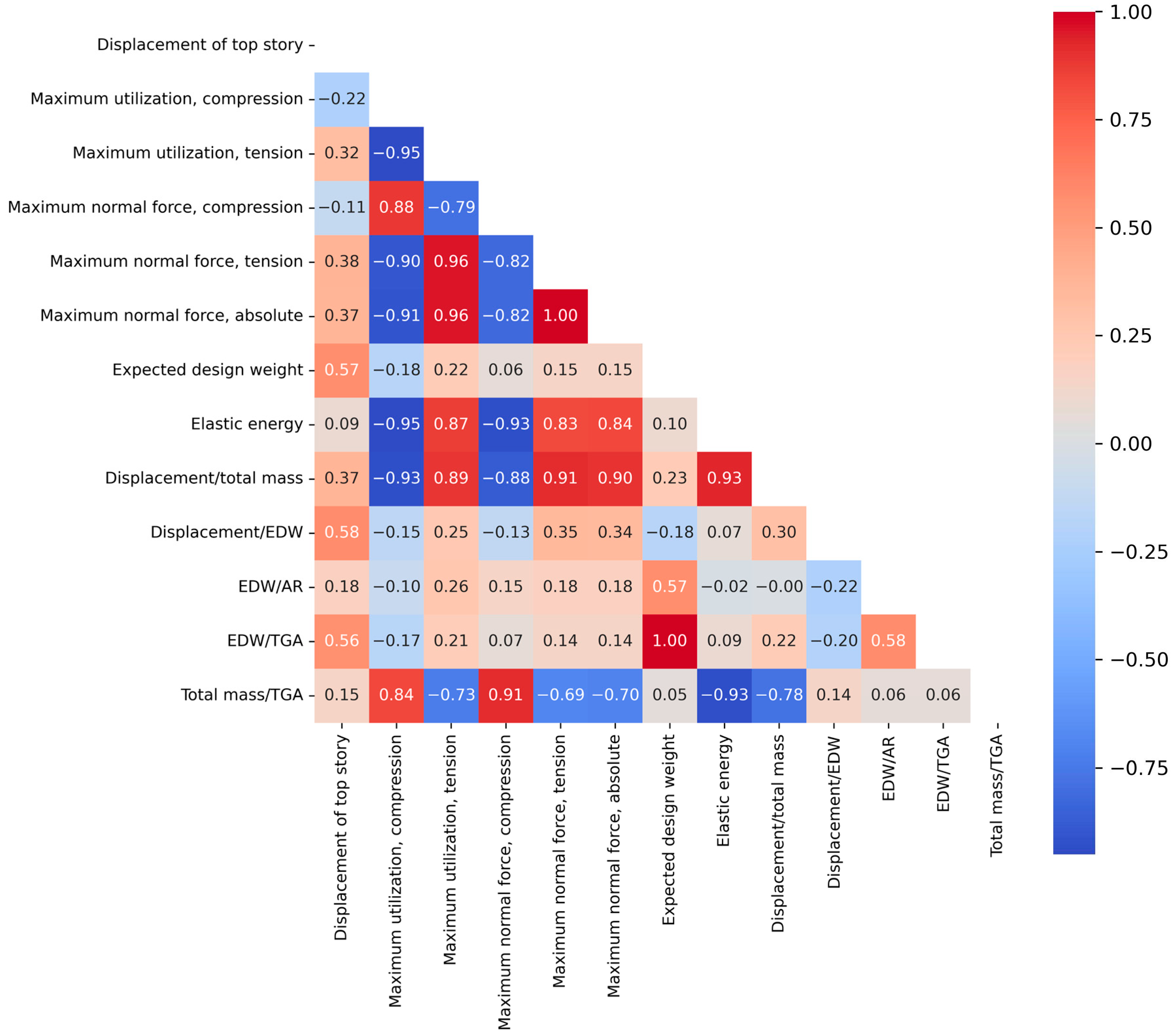
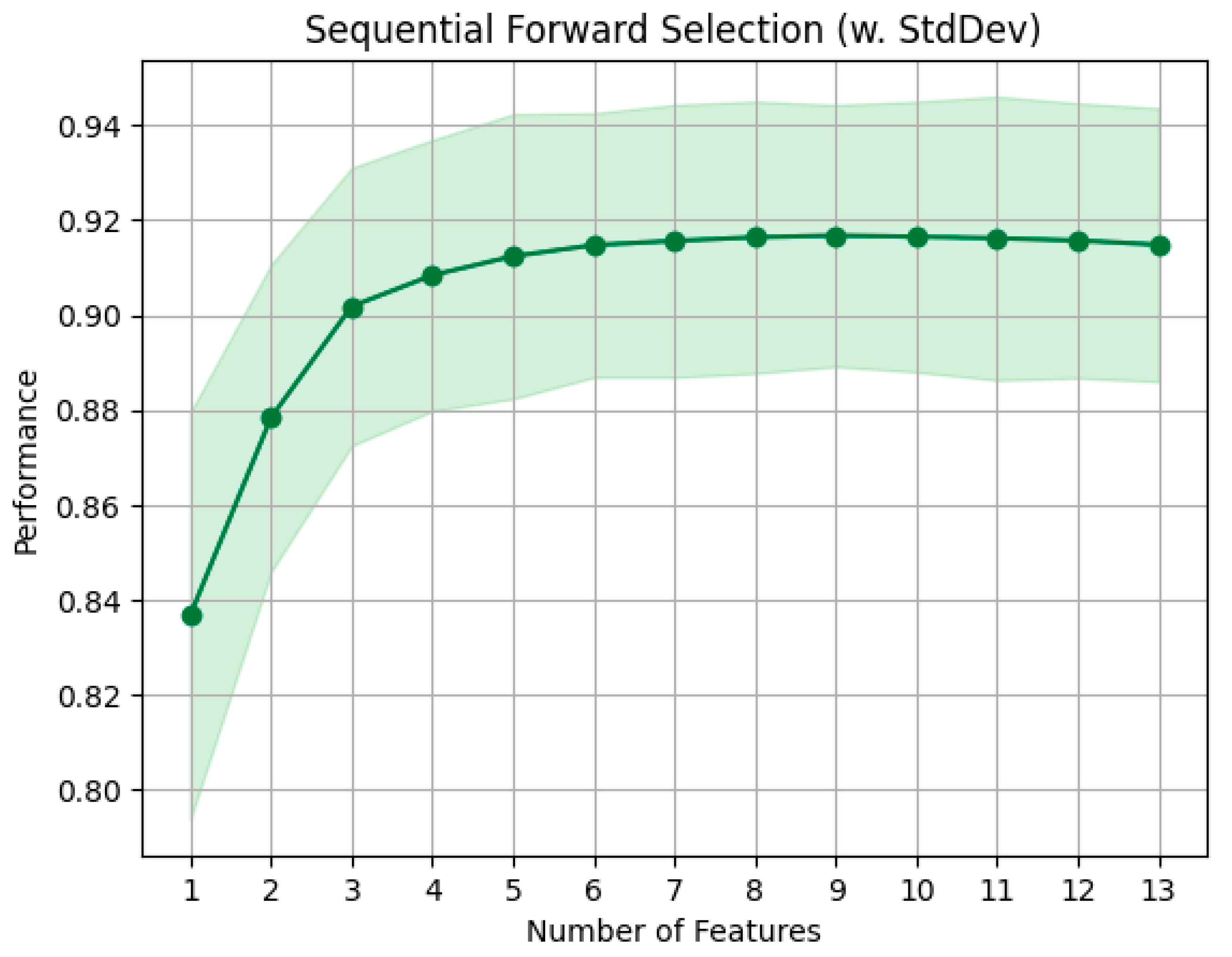
The outcome of this procedure is reported in Table 2. As the preferred number of features is dictated by optimal performance in the learning metric, the distinction between forward selection and backward elimination becomes negligible. The chosen assessment metric is the coefficient of determination (R2): a value close to 1 means superior performance, while values near zero suggest minimal distinction. The procedure of forward FS for a representative response (“displacement of top story”) is shown in Figure 4. It starts with one feature, achieving a coefficient of determination of 0.90. As the feature count increases to four, the optimal score of 0.93 is reached. Remarkably, adding up to nine features brings minimal change to the achieved score. Beyond this point, the learning score shows a decline as more features are incorporated. Both forward and backward methods end up being quite similar because the backward elimination reviews feature in the exact reverse order, making them essentially the same. Thus, only the forward method is used within this part of the study.
Table 2.
List of features selected through the forward method alongside their average cross-validation score.
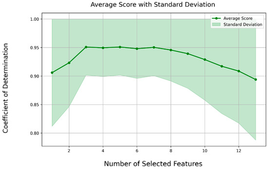
Figure 4.
FS performance analysis: variation in R2 and confidence interval via the forward selection method for the sample response “displacement of top story”.
To sum up, this method can pinpoint common features across different responses. When examining the designated features for each distinct response, it is clear that the “bottom plan side count” is consistently selected across most responses. Additionally, the “AR” feature is picked for four out of the five responses. Since these selected features are not very similar, it is wise to craft separate feature sets for each distinct response.
It is worthwhile underscoring that the “bottom plan side count” is selected in all methods, which emphasizes its pronounced significance in the FS process. On the other hand, the “top plan side count” is overlooked by both methods, indicating its limited relevance in this investigative framework.
5. Data Synthesis and Augmentation Algorithms
The combination of innovative architectural design concepts with limited data poses significant challenges. When ML tools are employed with small datasets, in fact, inconsistencies in results have been observed, as in our previous work [43], often attributed to the limited variation present in small data samples.
To mitigate this challenge, the use of synthetic data has been recommended by ML experts. This involves the generation of new data that mirrors the characteristics and patterns of the original dataset. In situations where original data is scarce, this synthetic data has been shown to enhance the accuracy of computer simulations and predictions. DA involves the alteration of existing data to introduce diversity without the creation of entirely new data points. In DA, this aim is achieved by diversifying representations while preserving the authenticity of the original dataset.
For the purposes of this research, focus has been placed on four specific algorithms renowned for their capability in data synthesis and augmentation including cross-validation: Gaussian copula (GC), conditional generative adversarial network (CGAN), Gaussian copula generative adversarial network (CGGAN), and variational autoencoder (VAE). These algorithms are implemented by using the synthetic data vault Python library [51], and the augmented dataset reaches 1200 data points, approximately an order of magnitude more than the original dataset. With respect to our previous work [43], focused only on GC-based DA in view of a classification task, here the mentioned four algorithms are used for a regressor. The aim is to check comparatively the quality of the DA in these alternatives.
Before executing the DA step, initial specifications about dataset metadata are needed, including the list of variables, their designated types, and subtypes. Moreover, relevant constraints are established to the variable values; for example, it is necessary to specify the number of sides in the top/bottom building plans, here set to a minimum of 3 up to a maximum of 24, and then to state the requirement for the overall building height, indicated as a multiple of the inter-floor 4 m height. Furthermore, the algorithm ensures that the synthesized data adheres to the boundaries of the original dataset. Not all columns from the original dataset are incorporated into the synthesizer algorithm: columns representing mathematical combinations of other variables are not required to be included in the synthesizer. Hence, an initial step involves the creation of a pruned dataset, which excludes such variables; subsequently, this trimmed dataset is utilized as input for the synthesizer; resulting in the generation of synthetic data with only the independent variables from both the original and synthetic datasets. During the evaluation phase, exclusively the independent variables from the original dataset and the synthetic dataset undergo comparison and rigorous analysis.
The architecture of the four aforementioned data synthesizers can be classified into two categories: statistics-based algorithms, exemplified by GC; and neural network-based algorithms, represented by CGAN, CGGAN, and VAE. A brief description of each algorithm is here reported for the sake of completeness.
The GC algorithm, characterized only by a few hyperparameters, is, for this reason, the first synthesizer considered here. It generates a multivariate Gaussian distribution; therefore, its output values are confined within the interval 0 ÷ 1. Conceptually, a copula is a mathematical construct that builds the joint distribution of different stochastic variables by exploring the relationships that exist between their individual marginal distributions [52]. In this work, Gaussian, gamma, beta, Student’s t, Gaussian-kde, and truncated-Gaussian distributions are assessed for each attribute within the dataset given DA. Original data values undergo a conversion into cumulative distribution function (CDF) values, based on their corresponding marginal distribution; then, an inverse CDF transformation, leveraging a standard normal distribution, is carried out. The correlations amidst these freshly generated stochastic variables are then computed and, subsequently, sampling is conducted from a multivariate standard normal distribution, factoring in the acquired correlations. Finally, a reversal procedure is pursued by reverting the sampled values to their standard normal CDF and applying an inverse CDF congruent with their individual marginal distributions [52].
The CGAN algorithm leverages the underlying mechanisms of generative adversarial networks (GANs) to augment datasets. In this paradigm, a pair of NNs, the generator, and the discriminator, compete one against the other (hence the “adversarial” attribute) towards a specific objective. In the case of DA, the generator component, by considering a subset of the original data for training, undertakes the task of crafting data that emulates the original dataset with an enhanced semblance; concurrently, the discriminator module assumes the responsibility of discerning between the artificially generated and authentic data, typically through a classification task exploiting a testing subset of the original data [50]. The process continues till the generator fools the discriminator into believing that the synthetic data agrees with the testing/original data.
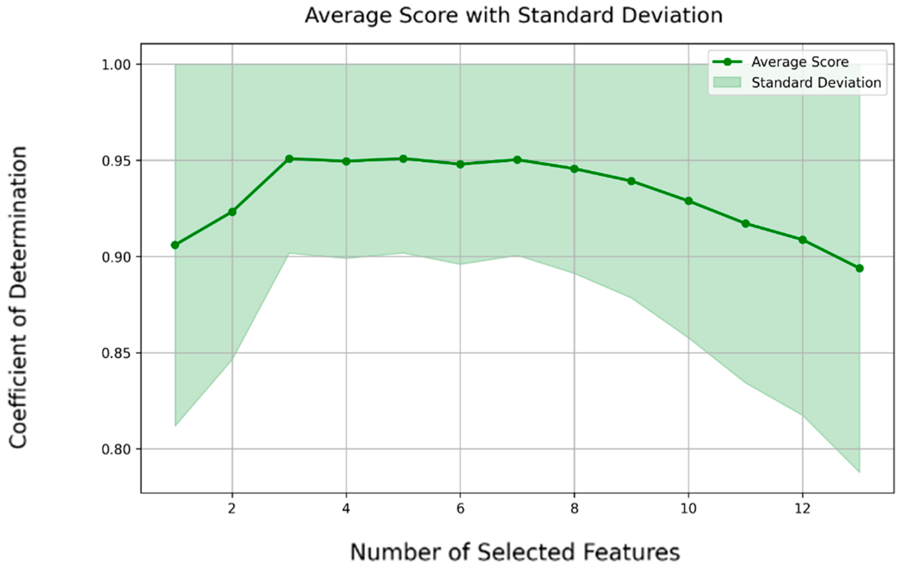
The CGGAN synthesis procedure is a kind of combination of the two previous methods, as it is carried out in two distinct stages: statistical learning, akin to the methodology employed by the GC algorithm, and GAN-based learning. This synthesizer starts by gaining an understanding of the marginal distributions inherent in the columns of real data and then subjects them to a normalization procedure. The normalized data undergoes a two-tiered training process utilizing the GAN framework [53]. A portrayal of the training progress is presented in Figure 5, displaying the dynamics of the generator and discriminator losses during the initial 10,000 epochs within a total training span of 50,000 epochs. A preliminary glance at this graphical representation might prompt queries regarding the oscillation of the discriminator’s loss value around 0. The behavior aligns with the inherently adversarial nature of NNs within GANs: as one constituent endeavors to enhance its performance, the opposing constituent must simultaneously elevate its capabilities to maintain equilibrium. In this case, the generator loss achieves stability at a negative value, while the discriminator loss remains consistently at 0: this equilibrium underscores the successful optimization of the generator, resulting in the creation of synthetic data that well mimics genuine data. The discriminator is incapable of distinguishing between the two, thereby corroborating the good performance of the GAN framework.
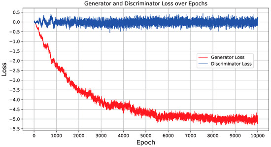
Figure 5.
Training progression of the CGAN synthesizer, highlighting the loss metrics for both discriminator and generator.
Finally, a VAE represents an NN architecture typically adopted in the domain of unsupervised learning, characterized by its encoder-decoder setup [50]. The former transforms input data into a concise latent space representation, whereas the latter reconstructs the original data from this latent representation. The distinguishing feature of VAEs resides in its incorporation of probabilistic modeling, wherein the encoder assimilates the capability to map input data onto a distribution within the latent space. This capacity empowers the generation of novel data instances through the process of sampling from this learned distribution. Throughout the training phase, the VAE framework aligns the acquired distribution with a predetermined simpler distribution. Consequently, a VAE emerges as inherently suited for the task of generating tabular data, as evidenced in numerous applications [50,53].
It is worth mentioning that the use of the last three algorithms, based on NNs, poses an initial challenge. The NN algorithm necessitates in fact a substantial volume of data for effective training, thereby casting doubt upon the capacity of these synthesizers to yield data akin to the original dataset. Additionally, their augmented complexity, as manifest in their array of hyperparameters with respect to the GC, underscores the complexities associated with their implementation. The endeavor to implement these synthesizers entails a process of hyperparameter tuning through iterative trial and error. This process is further underscored by the identification of critical hyperparameters that exert substantial influence on the outcomes. Illustratively, the epoch hyperparameter emerges as a paramount consideration. While akin research typically sets the epoch range at 1000 to 5000, this study deviates by necessitating a more substantial epoch count of 50,000 to achieve learning convergence and the generation of data with the highest semblance to the original dataset. Notably, elevating the epoch count to 100,000 does not yield appreciable enhancement in outcomes. Another pivotal hyperparameter, the batch size, is empirically defined through an iterative exploration of the synthesizing process. However, its impact is relatively subdued when compared to the epoch variable. While other hyperparameters are adjusted, their alteration yields either nominal improvements or, in some instances, leads to the generation of substandard data. Consequently, these hyperparameters are predominantly retained at their default values in the Mlxtend library.
To assess the fidelity of generated data, primarily the overall data quality, the conformity of column shapes, and the trend scores of column pairs for all four synthesizers are investigated. The results can be found in Table 3. Each of the synthesizers presents a very good quality level, surpassing 90%, a result demonstrating the effectiveness of the training processes in producing data of remarkable quality. The overall quality score is obtained by averaging two distinct scores, the column shape, and the column pair trend. The former is evaluated using the Kolmogorov–Smirnov complement metric [46,54], which quantifies the maximum discrepancy between the CDFs of the synthesized data and the authentic data, representing this difference within a numerical interval from 0 to 1. To indicate better data quality with a higher score, the Kolmogorov–Smirnov CDF is subtracted from 1 to provide this metric. The column pair trend score is based instead on the likeness of correlations between every column pair within the original dataset compared with the ones computed for each column pair within the augmented dataset. The correlations are based on Spearman’s rank correlation [46], i.e., the values in the two columns A and B are ranked from lowest to highest (becoming ρ(A) and ρ(B), respectively), then the index is computed as r = cov(ρ(A), ρ(B))/(σ(ρ(A))·σ(ρ(B))), being cov(·) and σ(·) the covariance and the standard deviation of the ranked values in the column, respectively. A value closer to one (100%) indicates the precise preservation of correlation between column pairs in the augmented dataset.
Table 3.
Quality assessment of synthetic data: percentage scores across four synthesizers.
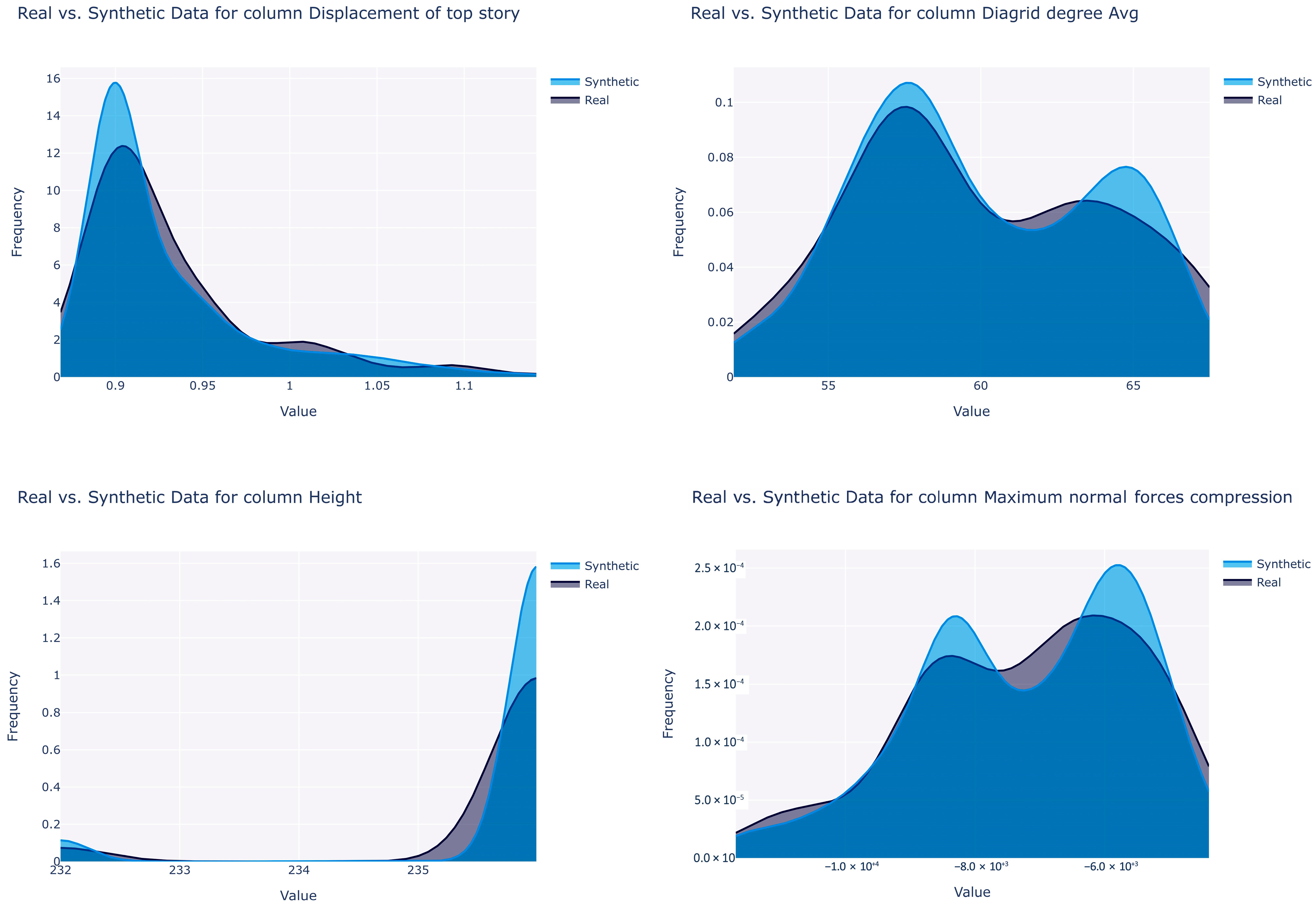
The GCGAN algorithm attains the highest overall quality score of 94.70%, while the lowest score is observed with VAE at 92.05%, though the difference between these scores remains marginal. GCGAN achieves the highest column shape score of 91.51%, while GC exhibits the lowest score at 86.5%. Interestingly, the impact of this parameter on the predictive model is not always straightforward. Figure 6 illustrates the probability density function of certain variables in the original and synthesized data by the GCGAN synthesizer. It is apparent that the boundaries are adhered to, preserving the column shapes. The corresponding column shape scores are notably elevated, with a value of 93.6% for “average diagrid degree”, 91.3% for “displacement of top story”, 93.5% for “maximum normal forces, compression”, and an exceptional score of 99.7% for “height”.

Figure 6.
Comparison of the synthetic vs. original data distributions for selected variables. (Top right) “average diagrid degree”, (top left) “displacement of top story”, (bottom right) “maximum normal forces, compression”, and (bottom left) “height”.
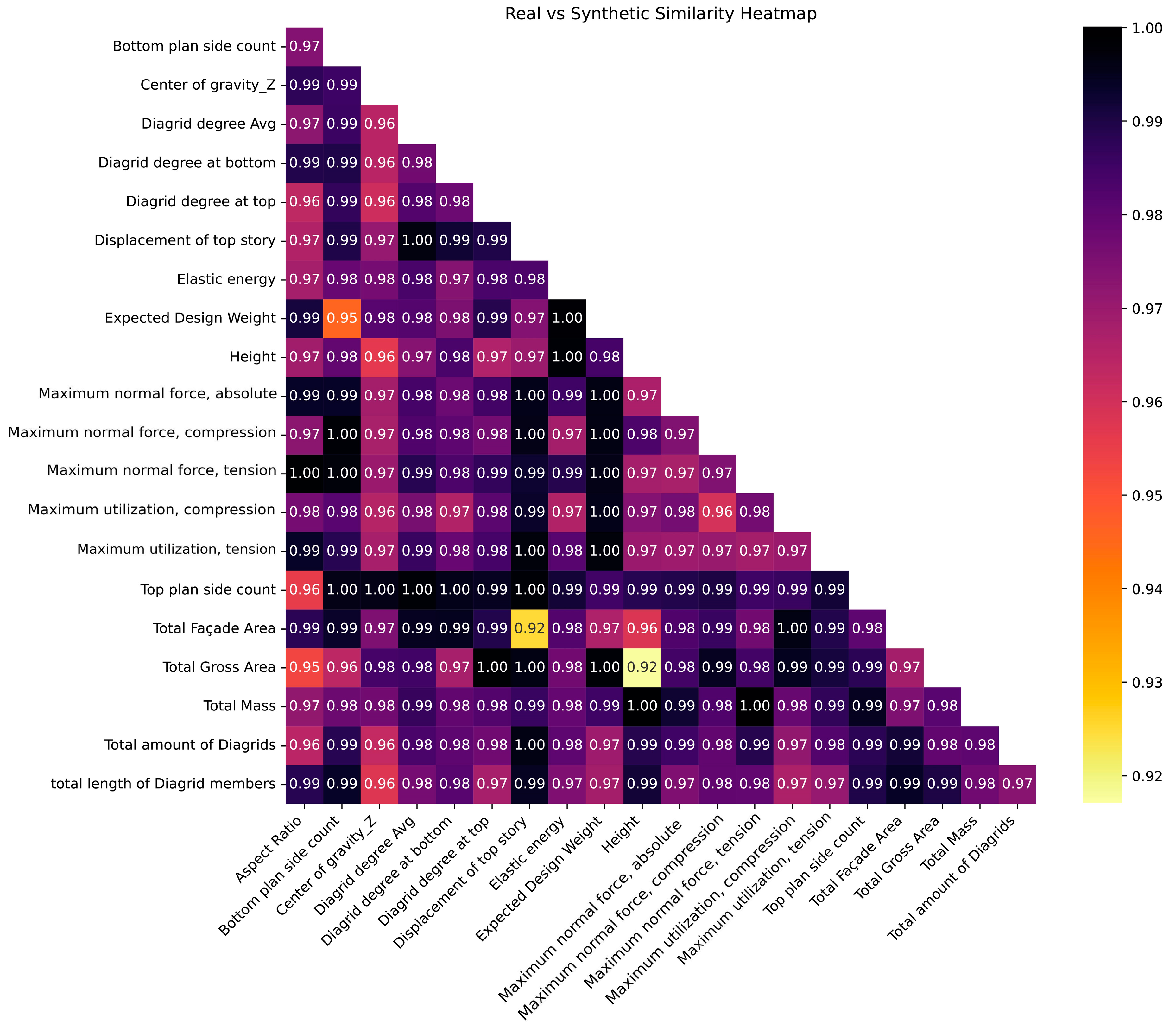
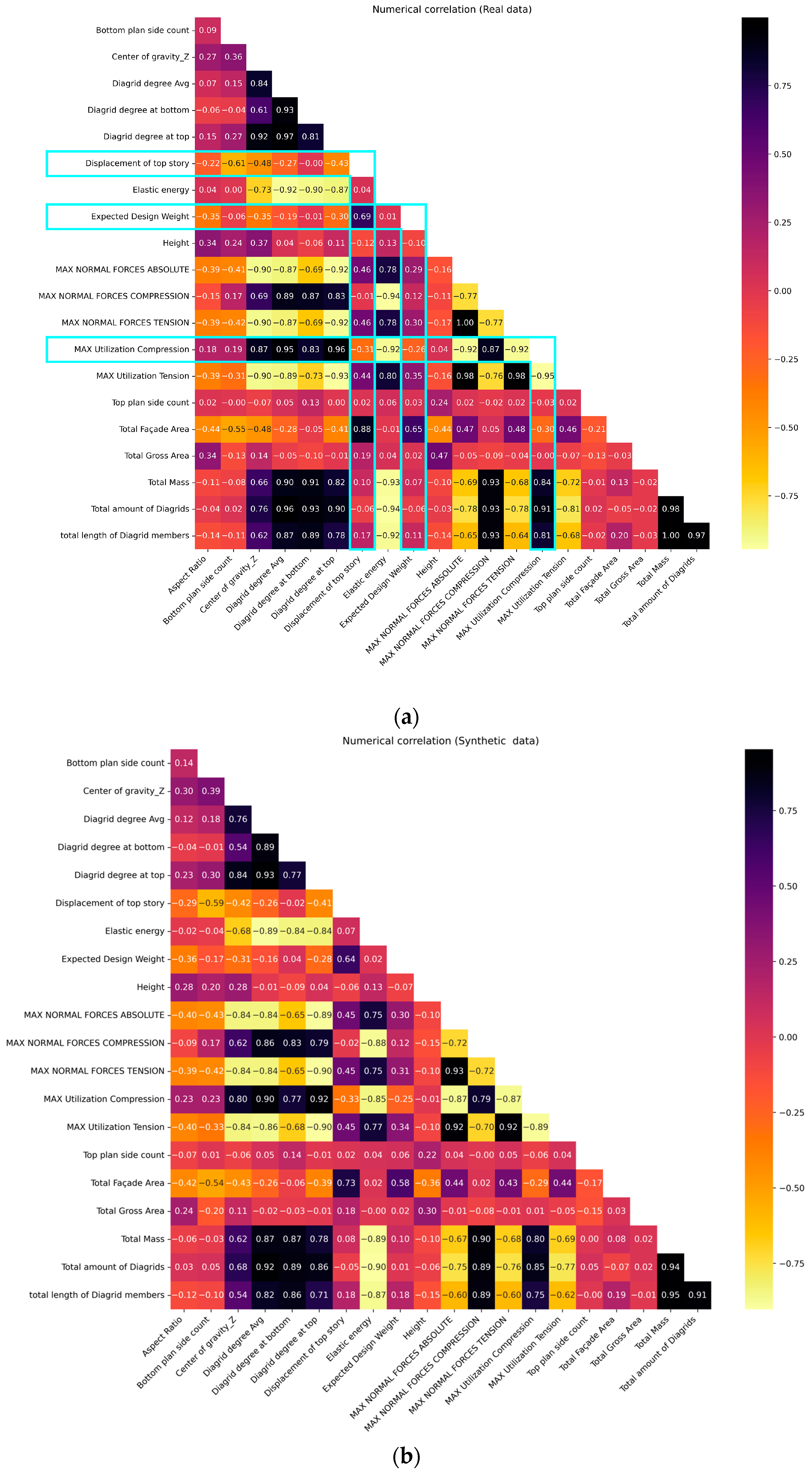
Revisiting Table 3, the highest column pair trend score is registered with GC at 98.66%, while the lowest score is associated with VAE at 95.52%, a minor disparity. The scores for all synthesizers indeed surpass the 95% threshold, indicating very good quality. The column pair trend score significantly influences the construction of predictive models; when the variables’ correlations are faithfully preserved, regression algorithms reveal comparable performance. Furthermore, the column pair trend heat map for GCGAN is visualized in Figure 7: it employs a color gradient ranging from black to yellow to visualize strongly correlated column pairs. Dark hues indicate a remarkably analogous correlation (i.e., approaching unity) between column pairs in both the original and synthesized data. Conversely, correlated column pairs represented by yellow shades depict lower correlations, but still higher than 0.91; hence, the overall result is quite good. For instance, the weakest correlation is observed between the “aspect ratio” and the “bottom plan side count”. Conversely, the highest correlation coefficient of 0.999 is unsurprisingly found between “total amount of diagrids” and “total length of diagrid members”. Further affirmation of the preservation of column correlations between the original and augmented datasets is evident when conducting a side-by-side comparison of the correlation matrices, as illustrated in Figure 8a and Figure 8b for the original and augmented datasets, respectively. These heat maps show aligned correlation patterns across almost all column pair relationships, further emphasizing the good quality of the synthetic data.
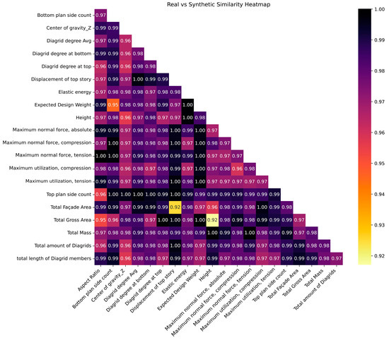
Figure 7.
Data augmentation: comparative correlation between the corresponding original/augmented column pairs.

Figure 8.
Data augmentation: feature/response reciprocal correlations for (a) original and (b) augmented dataset.
6. Regression Results
In this study, an RF regressor [55] was strategically employed to demonstrate the contribution of AI in structural and architectural engineering, specifically to determine the relationships between features and responses and to predict the output from a subset of input features after training. In the context of ML approaches, a regressor is not the only feasible choice for the problem at hand: alternatively, a classifier can be conveniently adopted, as shown in our previous work [43]. In a supervised learning framework, classification assigns each building to a class according to a predetermined set, while regression instead assigns a numerical value to a particular relationship between variables; the latter is used when most of the variables are real numbers, as in this case. While there are good reasons to use classification, as we stated in ref. [43], here we deliberately used regression analysis to show the soundness of our approach in this alternative as well. As will be shown, the outcome was qualitatively similar to what we already obtained in ref. [43] in terms of accuracy metrics for the five responses, with only a slight increase. Consequently, both classification and regression are valuable approaches to the problem at hand.
In view of a better training performance for the synthetic dataset, a 10-fold cross-validation technique was considered and the data was subjected to normalization. For the original, limited dataset, a high number of folds is a potential issue, because scattered data in a fold can distort the actual distribution, and instabilities in the results are therefore expected.
In analyzing the original data, the performance of the RF regressor exhibited notable variation across folds. For instance, R2 for the “displacement of top story” response fluctuates from 0.53 to 0.99 across different folds, yielding an average of 0.89. Furthermore, the RF regressor incorporates a random state variable and, when this variable was adjusted, performance outcomes varied: R2 score for a certain response ranged from 0.879 to 0.904, averaging 0.888, across 10 different random state settings. This marked instability underscores the non-uniformity of training performance for small datasets. Consequently, to ensure methodological rigor and to mitigate the influence of the random state variable, the average training performance between the 10 folds was considered in subsequent analyses.
Conversely, the training performance exhibited higher stability across various folds and random state variables when synthetic data was used, because a larger number of data points contributed to stabilizing the learning process. As an illustrative example, for the GCGAN synthetic data, the R2 score for the “displacement of top story” response varies from 0.66 to 0.82 across folds, with an average of 0.78. Similarly, the RF regressor’s performance varies based on different random state variables: R2 score ranges from 0.776 to 0.784, with an average of 0.781 for 10 different random state variables for the same response. Consequently, the accuracy among different folds and random states displays lower variation with respect to the original data, leading to enhanced stability in the learning process. To put it another way, these consistent outcomes highlighted the capability of AI to provide reliable results in complex engineering scenarios.
Table 4 presents the R2 scores for the original data (last two columns) and synthesized data (other columns) using the four aforementioned algorithms. Each synthesizer is initially trained with all features, then with the best-selected features for the synthetic data, and finally with the best-selected features but using the original data (Table 2). The use of different feature selection strategies on the synthesized data highlights the adaptability of AI in optimizing learning performance. It is worth noting that executing FS on the synthesized data instead of the original data gives a negligible improvement in learning performance, while it is computationally expensive, as it requires the creation of multiple RF models for each iteration, involving more feature combinations. In addition, this observation underscores the significance of AI in balancing computational efficiency and accuracy in engineering analysis. Figure 9 quantitatively illustrates the slight performance boost when the selected features increase from 4 to 13 for the “EDW/AR” response.
Table 4.
Coefficient of determination (R2) of the RF regressor. The results of four synthesized and original datasets are compared for different FS approaches. Negative values indicate an inverse correlation (For a clear visualization, results related to each synthesizer algorithm should be used with the same background color).
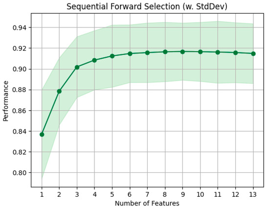
Figure 9.
Performance of the forward selection strategy on the “EDW/AR” response using the GCGAN-augmented dataset (The dotted lines represents the discreteness of number of features).
The R2 values notably decrease for the “EDW” and the “displacement/EDW” responses, sometimes also with negative values, indicating poor (inverse) correlation. If these two responses are excluded from the comparison, however, the remaining three exhibit a consistent behavior: R2 slightly increases by passing from including all the features to picking only the selected ones in Table 3, then the results slightly decrease if the procedure uses original instead of synthetic data. This pattern demonstrates the AI’s capacity to discern the most impactful features in a dataset, which is in general a key aspect in engineering optimizations. The variation in the regression model performance across different response variables, specifically the underperforming “EDW” and “displacement/EDW”, as opposed to the generally favorable performance with other response variables, stems from the inherent dataset correlations. Figure 8a visually captures these correlations with light blue rectangles showing the extent of correlation between variables.
For instance, the “maximum utilization compression” variable has a correlation value equal to the combined count of 13 cells in the horizontal rectangle and 7 cells in the vertical rectangle. In comparison to other response variables, “maximum utilization compression” exhibits the highest correlation values, approaching +1 or −1. This highlights that this variable, together with the “displacement of top story”, has the strongest correlations with other variables, while “EDW” displays instead the weakest correlations. When a response variable demonstrates a substantial correlation with other parameters, the regression performance remains consistent between the original and synthetic datasets. Conversely, for response variables such as “EDW” or “displacement/EDW”, which exhibit relatively weaker correlations with other parameters compared to other responses, noticeable performance differences emerge in synthetic data. The synthesizer algorithm operates by generating new data patterns based on variable correlations. When a variable displays strong correlations with other variables, the synthesizer reproduces values that closely resemble the original dataset. Conversely, variables with weaker correlations result in synthetic data that may significantly diverge from the original dataset. Essentially, the highest correlations are observed with “maximum utilization compression” and “displacement of the top story”, leading to the most accurate regressor performance on synthetic data. In contrast, consistently suboptimal performance is associated with “EDW” and “displacement/EDW”, characterized by lower correlations. Furthermore, the regressor demonstrates proficient performance on “EDW/AR”, primarily due to the inclusion of “AR” as one of its features. Therefore, it is important to emphasize that while all four synthesizers might have surprisingly high scores for column shape and column pair trends, this still does not guarantee satisfactory regressor performance for synthetic data.
Ultimately, the highest training performance is achieved by the GC synthesizer in three responses, while GCGAN excels in the two remaining responses. Conversely, the VAE synthesizer yields the lowest performance outcomes. This distinction in performance among different AI synthesizers underscores the importance of choosing the right AI tool for specific engineering applications. It is worthwhile mentioning that VAEs may struggle to capture complex, multi-modal distributions found in real-world tabular data, and they are often more suitable for capturing simpler data distributions. This insight into the capabilities of different AI technologies is crucial for their effective application in real-world engineering scenarios. In contrast, GANs are especially suitable for handling imbalanced datasets.
Table 5 shows the mean absolute percentage error (MAPE) of the regressor for the same different cases considered above for the R2 coefficient in Table 4. Attention is drawn to the divergence observed between the R2 and MAPE values in our modeling results. R2 values are indicative of the capacity of the model to explain the variance within the dataset, while MAPE values are reflective of the relative prediction errors.
Table 5.
Mean absolute percentage (%) error (MAPE) of the RF regressor. The results of four synthesized and original datasets are compared for different FS approaches (For a clear visualization, results related to each synthesizer algorithm should be used with the same background color).
It is recognized that the co-occurrence of high R2 and high MAPE can arise in scenarios where actual values have a limited range, or where a consistent bias is present in predictions across the data. Such occurrences do not reduce the validity of the model but highlight the complexities associated with predictive modeling.
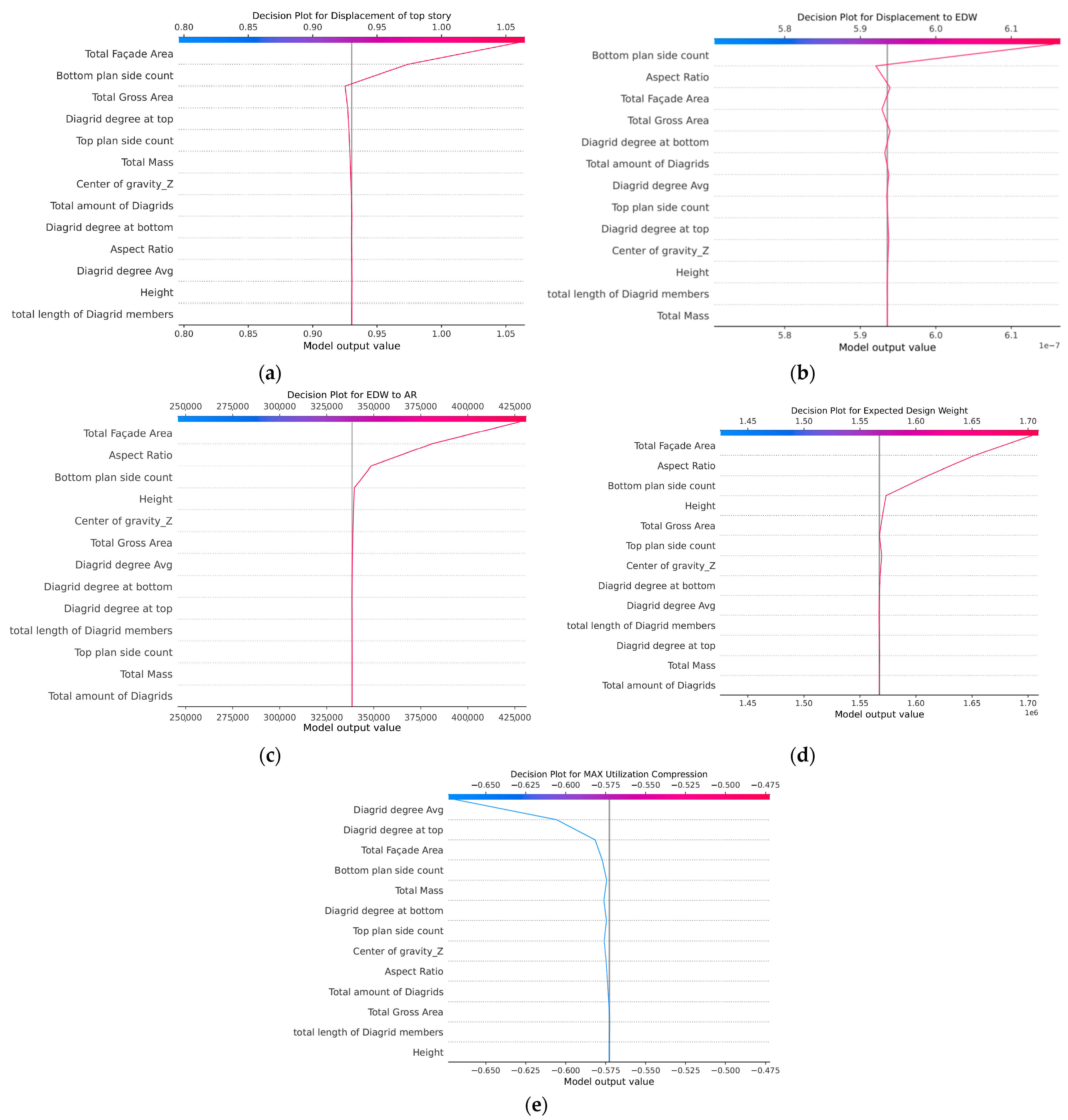
The role of the different features on the prediction capability related to each response can be appreciated by looking at the Shapley decision plots shown in Figure 10. In refs. [56,57], an approach based on game theory proposed a unified approach to explain the output of any ML model, called Shapley additive explanations (SHAP). To reflect how each feature contributes to an output prediction, an importance value is assigned. These SHAP values are based on Shapley values from cooperative game theory, where a total “payout” is fairly distributed among players based on their contributions to the game. The “payout” is interpreted in this context as the prediction output of the model, while the “players” are the features used by the model. In this way, the contribution of each feature to the five responses can be shown in Figure 10. For the first four responses, Figure 10a–d, the most important features for the prediction are the total façade area, the number of bottom sides, the aspect ratio, and, to a lesser extent, the height and the total gross area. The four responses are related to the overall behavior of the building, and it seems that in this case, the overall shape of the cantilever-like structure is mostly influencing the output. The response “max utilization (compression)”, Figure 10e, depends instead on the diagrid angle, both at the top and at the bottom, and again but less importantly from the total façade area and the number of bottom sides. It seems that, for this response which involves the local output for the structural elements in the diagrid, the relative angle between the elements in the diagrid matters the most, as evidenced in other studies [9,10].
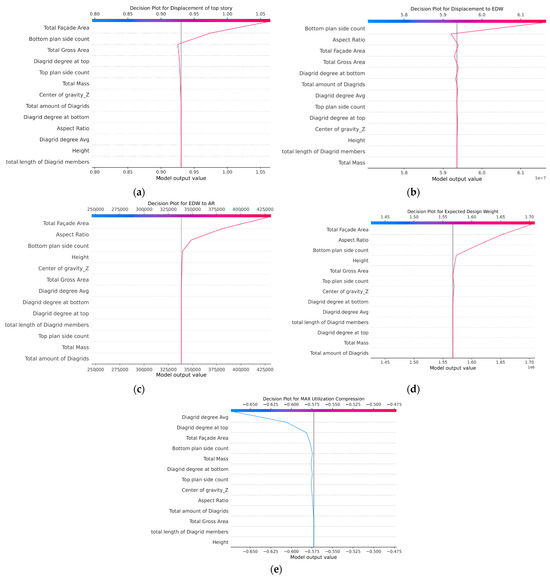
Figure 10.
SHAP decision plots for the five responses (a–e), showing the relevant contribution of the different features.
7. Conclusions
- In this study, the integral role of AI was underscored within the engineering domain, with a particular emphasis placed on its applicability in the early design stages of tall buildings incorporating outer diagrids. The proposed workflow addresses common AI challenges including the selection of optimal features and responses, management of limited dataset sizes, and attainment of stable learning accuracy.
- Employing a detailed FS process, both basic statistical correlations and sophisticated techniques such as forward selection and backward elimination were examined. This strategy confirmed that the selection of distinctive features from the original pool, rather than using a uniform set for all responses, is required to achieve good accuracy, see Table 2. This result is obviously relevant to architectural design, providing a means to support design decisions with quantifiable measurement derived from the machine learning (ML) methodology.
- The issue of dataset insufficiency was addressed by analyzing four distinct data synthesis algorithms to effectively enhance the dataset since generating a sufficiently large dataset is always a costly necessity for ML learning applications in architectural and structural design. As the quality of the synthetic data was rigorously evaluated through novel AI methodologies, although all the proposed algorithms performed reasonably well, the GCGAN achieved the highest overall quality score, while the VAE comparatively yielded the lowest score. It was ensured that these methodologies were validated with public datasets for replicability. In this work, the fidelity measurement was based on the AI’s application in preserving column shape and correlation trends, and on the subsequent learning capabilities of an RF regressor.
- A thorough assessment of data fidelity showcased the GC algorithm as particularly effective for synthesizing data across three crucial responses, primarily due to its computational efficiency and user-friendliness. On the other hand, the other three algorithms displayed greater complexity, demanding substantial hyperparameter tuning to generate high-quality data, often requiring an extensive number of epochs. Ultimately, by balancing quality score and ease of use, the GC has demonstrated the highest proficiency in synthesizing data for three responses, with GCGAN excelling in the remaining two. Conversely, VAE yielded comparatively inferior outcomes. Furthermore, the RF ML algorithm showed stable performance over a variety of cross-validation methods when tested on synthetic data, although a marginal decrease in the coefficient of determination on the augmented dataset versus the original must be acknowledged. The increased time efficiency and simplicity of this approach require attentive consideration by the designer in the context of AI’s application in engineering.
- The limitations due to the dataset’s size and diversity were acknowledged, highlighting the need for more comprehensive datasets to improve AI’s applicability in architectural design. Future work will aim to incorporate datasets generated from dynamic numerical simulations and explore alternative feature sampling methods, such as randomly generated floor plans or varying building heights selected by a Latin hypercube algorithm. These efforts will further demonstrate the methodological rigor and real-world application of AI in engineering.
Supplementary Materials
The following supporting information can be downloaded at: https://www.mdpi.com/article/10.3390/buildings14041118/s1.
Author Contributions
Conceptualization, P.K., A.G. and A.E.; methodology, P.K., A.G. and A.E.; software, P.K. and A.G.; validation, P.K. and A.G.; formal analysis, P.K., A.G. and A.E.; investigation, P.K., A.G. and A.E.; resources, P.K. and A.G.; data curation, P.K., A.G. and A.E.; writing—original draft preparation, P.K., A.G. and A.E.; writing—review and editing, P.K., A.G. and A.E.; visualization, P.K., A.G. and A.E.; supervision, A.G. and A.E.; project administration, P.K., A.G. and A.E. All authors have read and agreed to the published version of the manuscript.
Funding
This research received no external funding.
Data Availability Statement
The raw data supporting the conclusions of this article will be made available by the authors on request.
Conflicts of Interest
The authors declare no conflicts of interest.
References
- Farrar, C.R.; Worden, K. Structural Health Monitoring: A Machine Learning Perspective; John Wiley & Sons: Hoboken, NJ, USA, 2012. [Google Scholar]
- Hyde, R. Computer-Aided Architectural Design and The Design Process; Taylor & Francis: Abingdon, UK, 2016; pp. 255–256. [Google Scholar]
- Sun, H.; Burton, H.V.; Huang, H. Machine learning applications for building structural design and performance assessment: State-of-the-art review. J. Build. Eng. 2021, 33, 101816. [Google Scholar] [CrossRef]
- Zheng, H.; Moosavi, V.; Akbarzadeh, M. Machine learning assisted evaluations in structural design and construction. Autom. Constr. 2020, 119, 103346. [Google Scholar] [CrossRef]
- Özerol, G.; Arslan Selçuk, S. Machine learning in the discipline of architecture: A review on the research trends between 2014 and 2020. Int. J. Archit. Comput. 2023, 21, 23–41. [Google Scholar] [CrossRef]
- Brown, N.; De Oliveira, J.I.F.; Ochsendorf, J.; Mueller, C. Early-stage integration of architectural and structural performance in a parametric multi-objective design tool. In Proceedings of the 3rd Annual Conference on Structures and Architecture, Guimarães, Portugal, 27–29 July 2016; pp. 27–29. [Google Scholar]
- Elnimeiri, M.; Almusharaf, A. The interaction between sustainable structures and architectural form of tall buildings. Int. J. Sustain. Build. Technol. Urban Dev. 2010, 1, 35–41. [Google Scholar] [CrossRef]
- Park, S.M.; Elnimeiri, M.; Sharpe, D.C.; Krawczyk, R.J. Tall building form generation by parametric design process. In Proceedings of the CTBUH 2004 Conference, Seoul, Republic of Korea, 10–13 October 2004; pp. 10–13. [Google Scholar]
- Asadi, E.; Salman, A.M.; Li, Y. Multi-criteria decision-making for seismic resilience and sustainability assessment of diagrid buildings. Eng. Struct. 2019, 191, 229–246. [Google Scholar] [CrossRef]
- Scaramozzino, D.; Albitos, B.; Lacidogna, G.; Carpinteri, A. Selection of the optimal diagrid patterns in tall buildings within a multi-response framework: Application of the desirability function. J. Build. Eng. 2022, 54, 104645. [Google Scholar] [CrossRef]
- Ali, M.M.; Al-Kodmany, K. Tall buildings and urban habitat of the 21st century: A global perspective. Buildings 2012, 2, 384–423. [Google Scholar] [CrossRef]
- Kazemi, P.; Afghani, R.; Tahcildoost, M. Investigating the effect of architectural form on the structural response of lateral loads on diagrid structures in tall buildings. In Proceedings of the 5th International Conference on Architecture and Built Environment with AWARDs Book of Abstracts, Venice, Italy, 22–24 May 2018; pp. 25–34. [Google Scholar]
- Khoraskani, R.; Kazemi, P.; Tahsildoost, M. Adaptation of Hyperboloid Structure for High-Rise Buildings with Exoskeleton. In Proceedings of the 5th International Conference on Architecture and Built Environment with AWARDs Book of Abstracts, Venice, Italy, 22–24 May 2018; pp. 62–71. [Google Scholar]
- Ali, M.M.; Moon, K.S. Advances in structural systems for tall buildings: Emerging developments for contemporary urban giants. Buildings 2018, 8, 104. [Google Scholar] [CrossRef]
- Danhaive, R.; Mueller, C.T. Design subspace learning: Structural design space exploration using performance-conditioned generative modeling. Autom. Constr. 2021, 127, 103664. [Google Scholar] [CrossRef]
- Yazici, S. A machine-learning model driven by geometry, material and structural performance data in architectural design process. In Proceedings of the 38th eCAADe Conference, Berlin, Germany, 16–17 September 2020; pp. 16–18. [Google Scholar]
- As, I.; Pal, S.; Basu, P. Artificial intelligence in architecture: Generating conceptual design via deep learning. Int. J. Archit. Comput. 2018, 16, 306–327. [Google Scholar] [CrossRef]
- Abioye, S.O.; Oyedele, L.O.; Akanbi, L.; Ajayi, A.; Delgado, J.M.; Bilal, M.; Akinade, O.O.; Ahmed, A. Artificial intelligence in the construction industry: A review of present status, opportunities and future challenges. J. Build. Eng. 2021, 44, 103299. [Google Scholar] [CrossRef]
- Nguyen, P.T. Application machine learning in construction management. TEM J. 2021, 10, 1385–1389. [Google Scholar] [CrossRef]
- Huang, Y.; Fu, J. Review on application of artificial intelligence in civil engineering. Comput. Model. Eng. Sci. 2019, 3, 845–875. [Google Scholar] [CrossRef]
- Preisinger, C. Linking structure and parametric geometry. Archit. Des. 2013, 83, 110–113. [Google Scholar] [CrossRef]
- Akinosho, T.D.; Oyedele, L.O.; Bilal, M.; Ajayi, A.O.; Delgado, M.D.; Akinade, O.O.; Ahmed, A.A. Deep learning in the construction industry: A review of present status and future innovations. J. Build. Eng. 2020, 32, 101827. [Google Scholar] [CrossRef]
- Ekici, B.; Kazanasmaz, Z.T.; Turrin, M.; Taşgetiren, M.F.; Sariyildiz, I.S. Multi-zone optimisation of high-rise buildings using artificial intelligence for sustainable metropolises. Part 1: Background, methodology, setup, and machine learning results. Sol. Energy 2021, 224, 373–389. [Google Scholar] [CrossRef]
- Luo, H.; Paal, S.G. Artificial intelligence-enhanced seismic response prediction of reinforced concrete frames. Adv. Eng. Inform. 2022, 52, 101568. [Google Scholar] [CrossRef]
- Paal, S.G.; Jeon, J.S.; Brilakis, I.; DesRoches, R. Automated damage index estimation of reinforced concrete columns for post-earthquake evaluations. J. Struct. Eng. 2015, 141, 04014228. [Google Scholar] [CrossRef]
- Entezami, A.; Shariatmadar, H.; Mariani, S. Fast unsupervised learning methods for structural health monitoring with large vibration data from dense sensor networks. Struct. Health Monit. 2020, 19, 1685–1710. [Google Scholar] [CrossRef]
- Rezaiee-Pajand, M.; Entezami, A.; Shariatmadar, H. An iterative order determination method for time-series modeling in structural health monitoring. Adv. Struct. Eng. 2018, 21, 300–314. [Google Scholar] [CrossRef]
- Entezami, A.; Shariatmadar, H.; Karamodin, A. Improving feature extraction via time series modeling for structural health monitoring based on unsupervised learning methods. Sci. Iran. 2020, 27, 1001–1018. [Google Scholar]
- Entezami, A.; Sarmadi, H.; Behkamal, B.; Mariani, S. Health monitoring of large-scale civil structures: An approach based on data partitioning and classical multidimensional scaling. Sensors 2021, 21, 1646. [Google Scholar] [CrossRef] [PubMed]
- Entezami, A.; Sarmadi, H.; Behkamal, B. A novel double-hybrid learning method for modal frequency-based damage assessment of bridge structures under different environmental variation patterns. Mech. Syst. Signal Process. 2023, 201, 110676. [Google Scholar] [CrossRef]
- Entezami, A.; Shariatmadar, H.; Mariani, S. Early damage assessment in large-scale structures by innovative statistical pattern recognition methods based on time series modeling and novelty detection. Adv. Eng. Softw. 2020, 150, 102923. [Google Scholar] [CrossRef]
- Hegde, J.; Rokseth, B. Applications of machine learning methods for engineering risk assessment—A review. Saf. Sci. 2020, 122, 104492. [Google Scholar] [CrossRef]
- Vadyala, S.R.; Betgeri, S.N.; Matthews, J.C.; Matthews, E. A review of physics-based machine learning in civil engineering. Results Eng. 2022, 13, 100316. [Google Scholar] [CrossRef]
- Yüksel, N.; Börklü, H.R.; Sezer, H.K.; Canyurt, O.E. Review of artificial intelligence applications in engineering design perspective. Eng. Appl. Artif. Intell. 2023, 118, 105697. [Google Scholar] [CrossRef]
- Junda, E.; Málaga-Chuquitaype, C.; Chawgien, K. Interpretable machine learning models for the estimation of seismic drifts in CLT buildings. J. Build. Eng. 2023, 70, 106365. [Google Scholar] [CrossRef]
- Zhou, K.; Xie, D.-L.; Xu, K.; Zhi, L.-H.; Hu, F.; Shu, Z.-R. A machine learning-based stochastic subspace approach for operational modal analysis of civil structures. J. Build. Eng. 2023, 76, 107187. [Google Scholar] [CrossRef]
- Meng, S.; Zhou, Y.; Gao, Z. Refined self-attention mechanism based real-time structural response prediction method under seismic action. Eng. Appl. Artif. Intell. 2024, 129, 107380. [Google Scholar] [CrossRef]
- Zhou, Y.; Meng, S.; Lou, Y.; Kong, Q. Physics-Informed Deep Learning-Based Real-Time Structural Response Prediction Method. Engineering, 2023; in press. [Google Scholar]
- Kazemi, F.; Asgarkhani, N.; Jankowski, R. Predicting seismic response of SMRFs founded on different soil types using machine learning techniques. Eng. Struct. 2023, 274, 114953. [Google Scholar] [CrossRef]
- Kazemi, P.; Ghisi, A.; Mariani, S. Classification of the Structural Behavior of Tall Buildings with a Diagrid Structure: A Machine Learning-Based Approach. Algorithms 2022, 15, 349. [Google Scholar] [CrossRef]
- Aha, D.W.; Bankert, R.L. A comparative evaluation of sequential feature selection algorithms. In Proceedings of the 5th International Workshop on Artificial Intelligence and Statistics—PMLR, Fort Lauderdale, FL, USA, 4–7 January 1995; pp. 1–7. [Google Scholar]
- Guyon, I.; Elisseeff, A. An introduction to variable and feature selection. J. Mach. Learn. Res. 2003, 3, 1157–1182. [Google Scholar]
- Kazemi, P.; Entezami, A.; Ghisi, A. Machine-learning techniques for diagrid building design: Architectural-Structural correlations with feature selection and data augmentation. J. Build. Eng. 2024, 86, 108766. [Google Scholar] [CrossRef]
- Alauthman, M.; Al-Qerem, A.; Sowan, B.; Alsarhan, A.; Eshtay, M.; Aldweesh, A.; Aslam, N. Enhancing Small Medical Dataset Classification Performance Using GAN. Informatics 2023, 10, 28. [Google Scholar] [CrossRef]
- Mumuni, A.; Mumuni, F. Data augmentation: A comprehensive survey of modern approaches. Array 2022, 16, 100258. [Google Scholar] [CrossRef]
- Corder, G.W.; Foreman, D.I. Nonparametric Statistics: A Step-by-Step Approach; John Wiley & Sons: Hoboken, NJ, USA, 2014. [Google Scholar]
- Zar, J.H. Significance testing of the Spearman rank correlation coefficient. J. Am. Stat. Assoc. 1972, 67, 578–580. [Google Scholar] [CrossRef]
- Tjøstheim, D.; Otneim, H.; Støve, B. Statistical Modeling Using Local Gaussian Approximation; Academic Press: Cambridge, MA, USA, 2021. [Google Scholar]
- Raschka, S. Mlxtend: Providing machine learning and data science utilities and extensions to Python’s scientific computing stack. J. Open Source Softw. 2018, 3, 638. [Google Scholar] [CrossRef]
- Bemister-Buffington, J.; Wolf, A.J.; Raschka, S.; Kuhn, L.A. Machine learning to identify flexibility signatures of class a GPCR inhibition. Biomolecules 2020, 10, 454. [Google Scholar] [CrossRef]
- Alizadeh, E. Synthetic Data Vault (SDV): A Python Library for Dataset Modeling. Available online: https://ealizadeh.com/blog/sdv-library-for-modeling-datasets (accessed on 15 December 2023).
- Li, Z.; Zhao, Y.; Fu, J. Sync: A copula based framework for generating synthetic data from aggregated sources. In Proceedings of the International Conference on Data Mining Workshops (ICDMW), Sorrento, Italy, 17–20 November 2020; pp. 571–578. [Google Scholar]
- Xu, L.; Skoularidou, M.; Cuesta-Infante, A.; Veeramachaneni, K. Modeling tabular data using conditional GAN. In Proceedings of the 33rd Conference on Neural Information Processing Systems (NeurIPS 2019), Vancouver, BC, Canada, 8–14 December 2019. [Google Scholar]
- Massey, F.J., Jr. The Kolmogorov-Smirnov test for goodness of fit. J. Am. Stat. Assoc. 1951, 46, 68–78. [Google Scholar] [CrossRef]
- Chen, Q.; Zhang, X.; Wang, Y.; Zhai, Z.; Yang, F. Applying a Random Forest Approach to Imbalanced Dataset on Network Monitoring Analysis. In China Cyber Security Annual Conference; Springer Nature: Singapore, 2022; pp. 28–37. [Google Scholar]
- Lundberg, S.M.; Lee, S.-I. A unified approach to interpreting model predictions. Adv. Neural Inf. Process. Syst. 2017, 30, 4765–4774. [Google Scholar]
- Shafighfard, T.; Kazemi, F.; Bagherzadeh, F.; Mieloszyk, M.; Yoo, D.Y. Chained machine learning model for predicting load capacity and ductility of steel fiber–reinforced concrete beams. Comput. Aided Civ. Infrastruct. Eng. 2024; in press. [Google Scholar]
Disclaimer/Publisher’s Note: The statements, opinions and data contained in all publications are solely those of the individual author(s) and contributor(s) and not of MDPI and/or the editor(s). MDPI and/or the editor(s) disclaim responsibility for any injury to people or property resulting from any ideas, methods, instructions or products referred to in the content. |
© 2024 by the authors. Licensee MDPI, Basel, Switzerland. This article is an open access article distributed under the terms and conditions of the Creative Commons Attribution (CC BY) license (https://creativecommons.org/licenses/by/4.0/).