

Imperfection Sensitivity Detection in Pultruded Columns Using Machine Learning and Synthetic Data


Abstract
1. Introduction
2. Materials and Methods
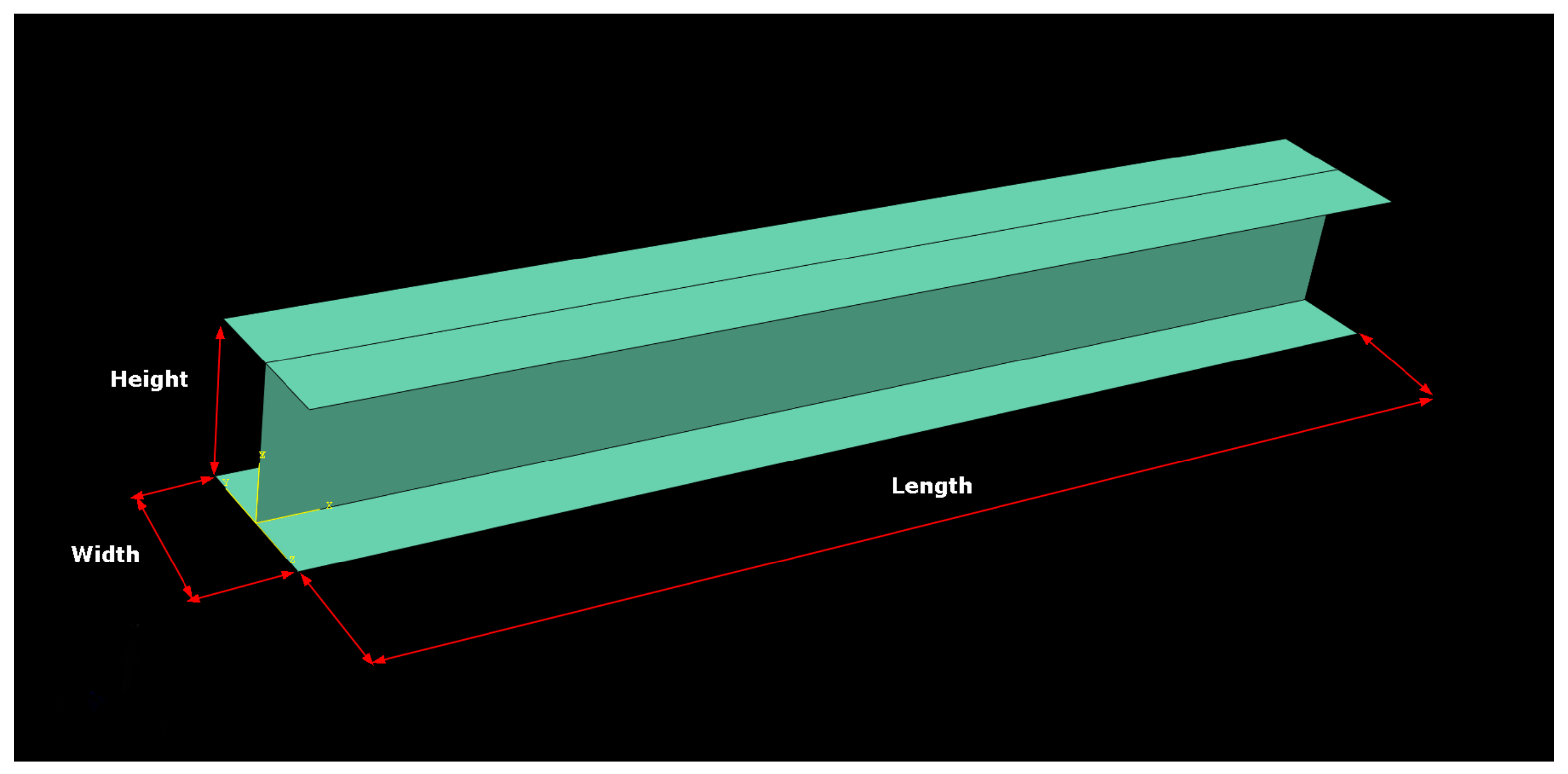
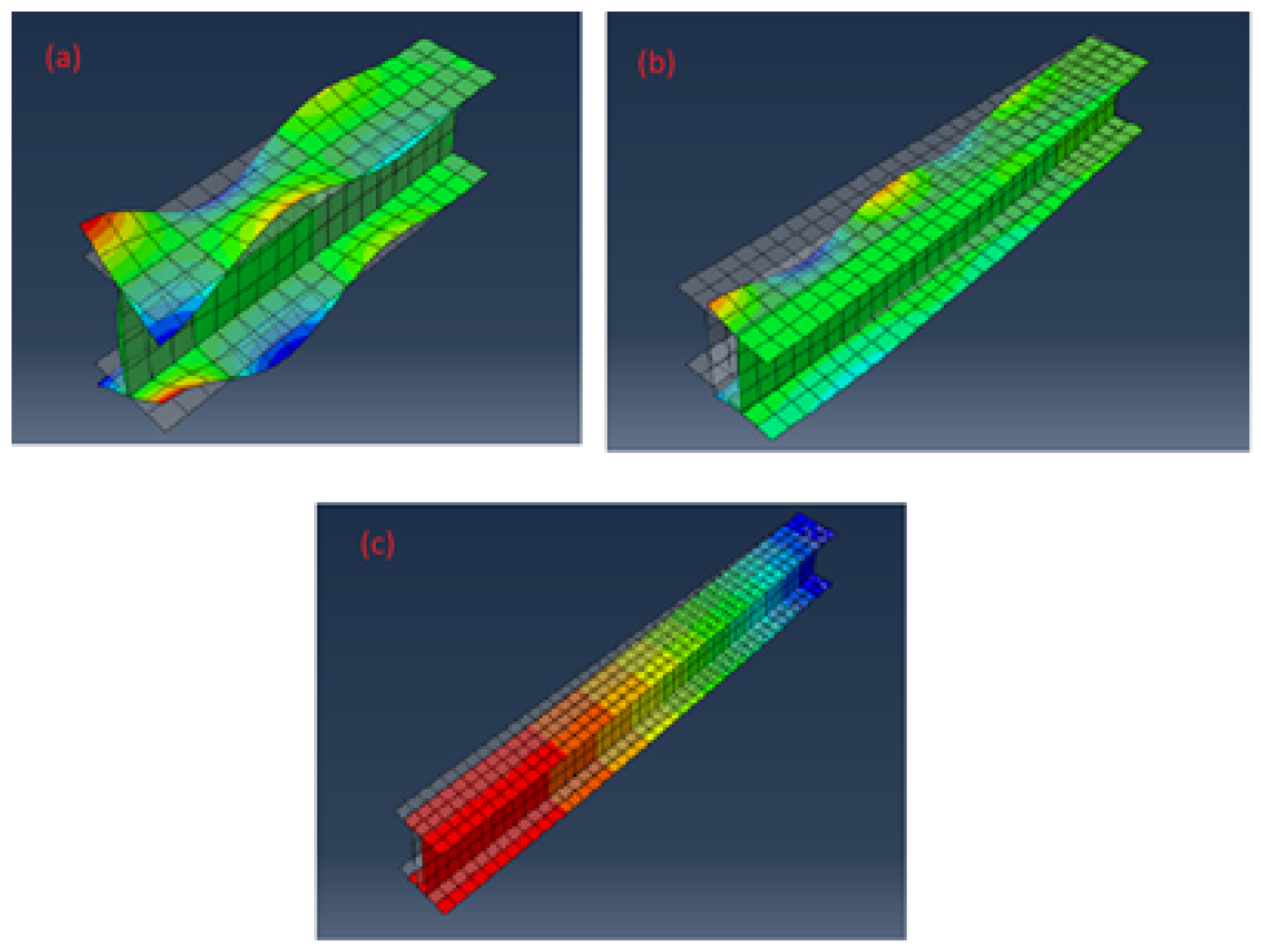
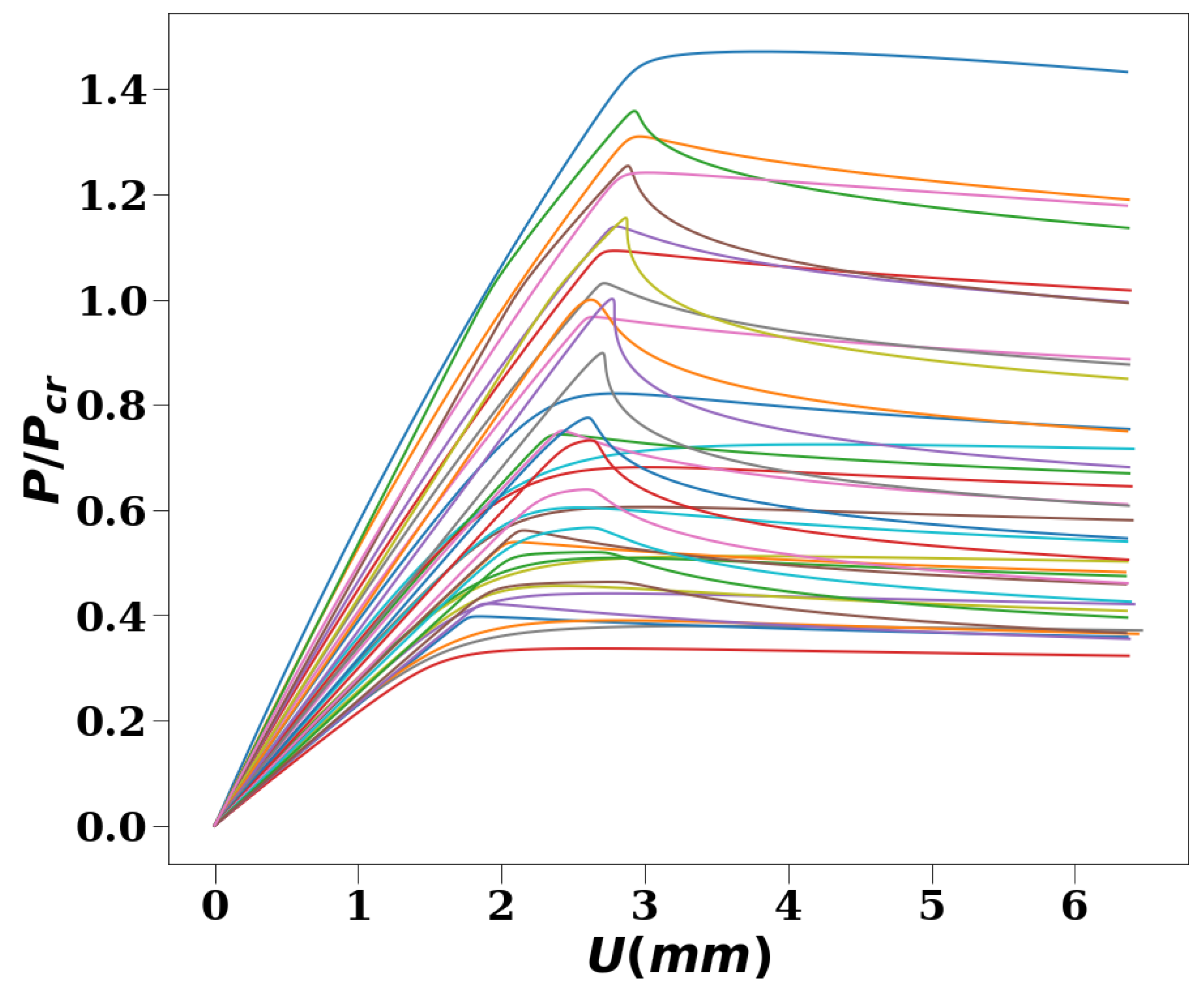
2.1. Case Study of a Pultruded Column: Finite Element Simulation Data Acquisition
2.2. Machine Learning Model
2.3. Finite Element Simulations and Feature Selection
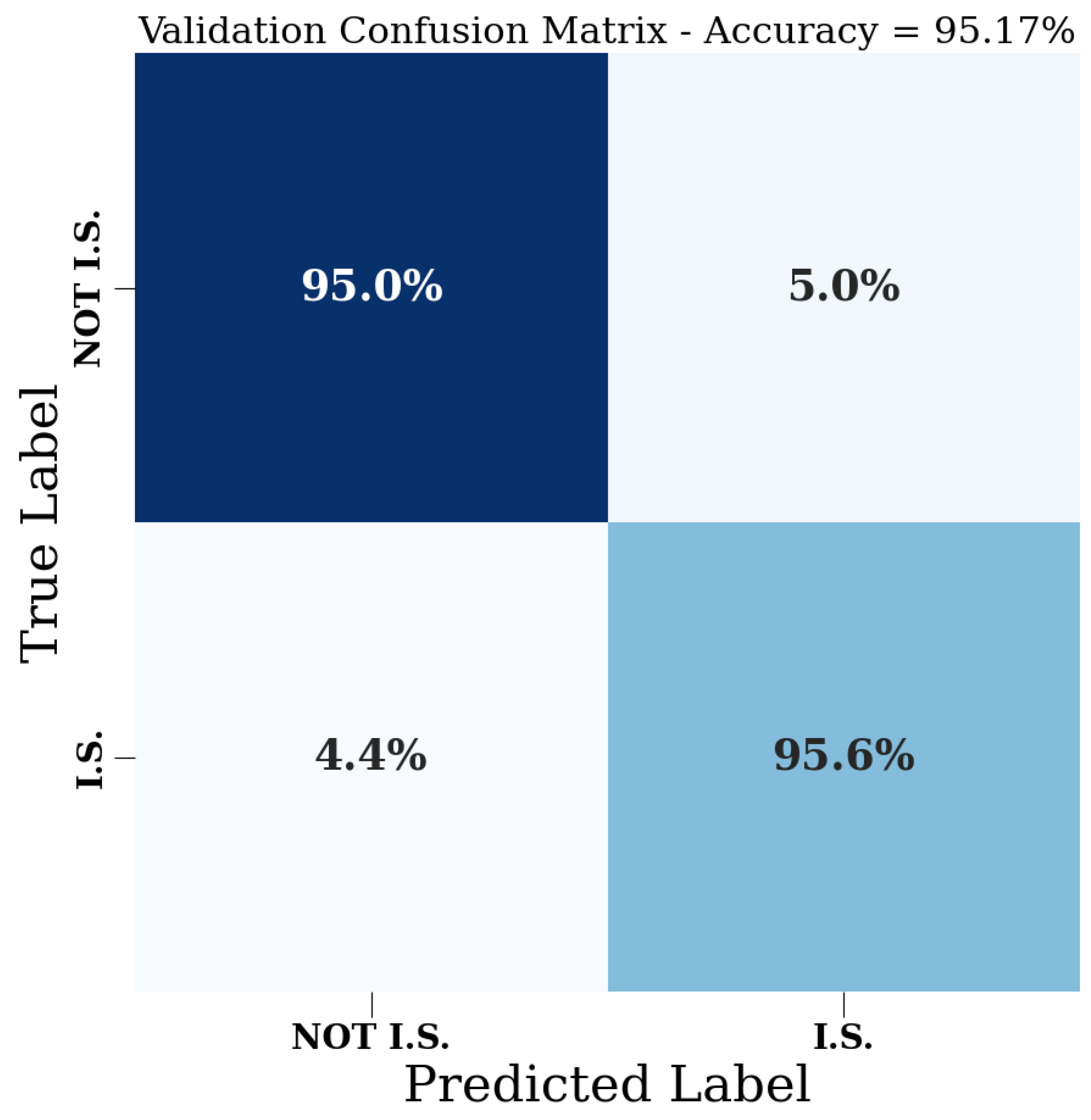
3. Results
4. Discussion
Author Contributions
Funding
Data Availability Statement
Acknowledgments
Conflicts of Interest
Abbreviations
| ML | Machine learning |
| SHM | Structural health monitoring |
| FEA | Finite Element Analysis |
| FRP | Fiber-reinforced plastic |
| WF | Wide flange |
| IS | Imperfection-sensitive |
| NIS | Non-imperfection-sensitive |
| NGA | Non-linear geometric analysis |
| AI | Artificial Intelligence |
| NN | Neural network |
| MLP | Multilayer perceptron |
| RP | Reference point |
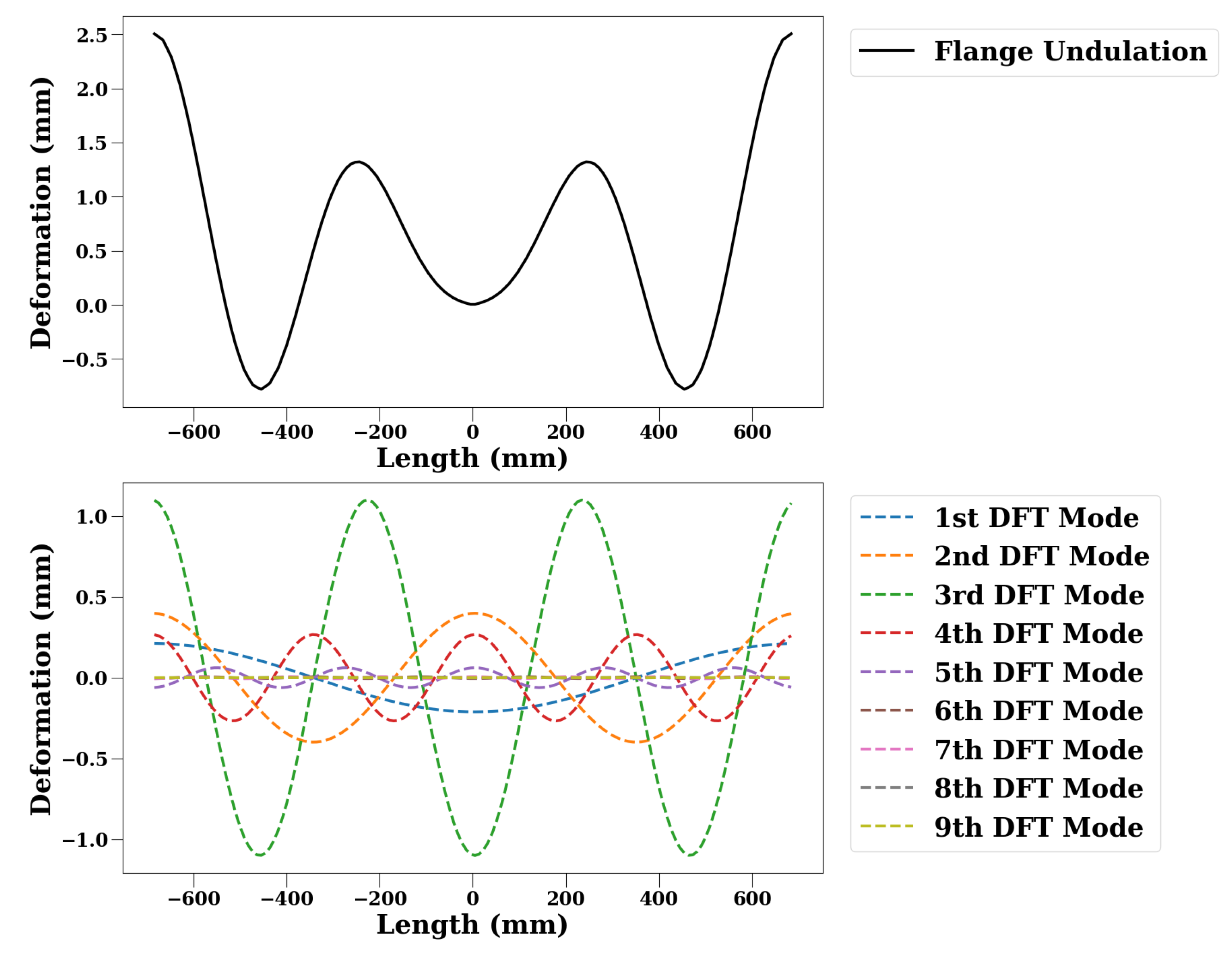
| DFT | Discrete Fourier transform |
| FFT | Fast Fourier Transform |
| SVM | Support Vector Machine |
| Symbols | |
| Slenderness of a column, ratio of column length over critical length | |
| Local buckling load | |
| Euler buckling load | |
| L | Column length |
| Column critical length | |
| E | Young’s modulus |
| I | Second moment of inertia for the cross-section |
| K | Parameter that changes based on end-supports of a column |
| Column critical load | |
| N | Total number of samples |
| Column peak load | |
| Column final load | |
| Column final displacement | |
| Column displacement at peak load |
References
- Bonopera, M.; Chang, K.C.; Chen, C.C.; Lin, T.K.; Tullini, N. Compressive column load identification in steel space frames using second-order deflection-based methods. Int. J. Struct. Stab. Dyn. 2018, 18, 1850092. [Google Scholar] [CrossRef]
- Dassault Systèmes. Abaqus 2020 Documentation. 2020. Available online: https://www.3ds.com/ (accessed on 1 April 2024).
- Barbero, E.J. Buckling Mode Interaction in Pultruded Composite Columns. YouTube. 2019. Available online: https://youtu.be/Nl8YRFQMcfg (accessed on 1 April 2024).
- Eidukynas, D.; Adumitroaie, A.; Griškevičius, P.; Grigaliunas, V.; Vaitkūnas, T. Finite Element Model Updating Approach for Structural Health Monitoring of Lightweight Structures Using Response Surface Optimization. In Proceedings of the IOP Conference Series: Materials Science and Engineering; IOP Publishing: Bristol, UK, 2022; Volume 1239, p. 012002. [Google Scholar]
- Budiansky, B. Theory of buckling and post-buckling behavior of elastic structures. Adv. Appl. Mech. 1974, 14, 1–65. [Google Scholar]
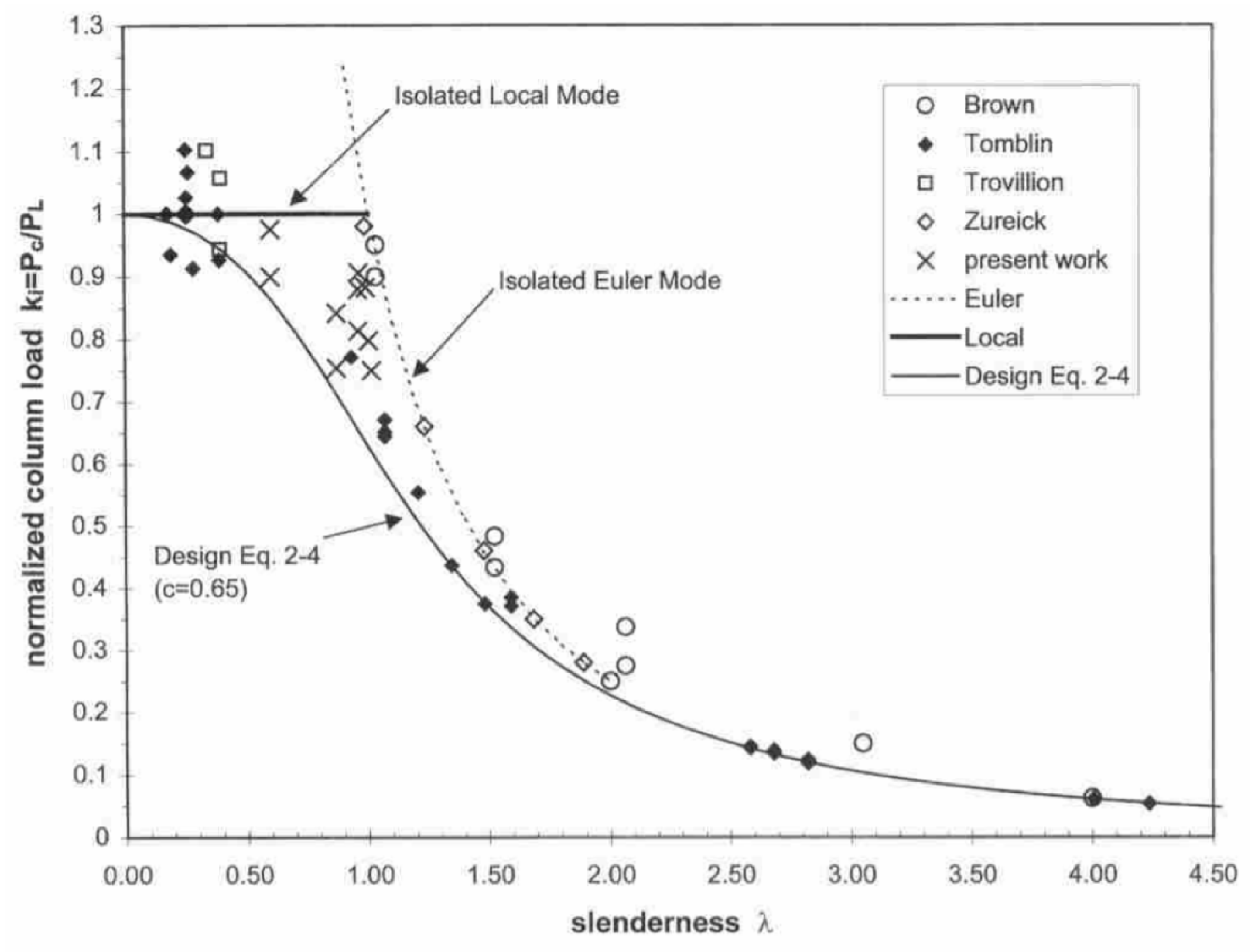
- Barbero, E.; Tomblin, J. A phenomenological design equation for FRP columns with interaction between local and global buckling. Thin-Walled Struct. 1994, 18, 117–131. [Google Scholar] [CrossRef]
- Ascione, F.; Feo, L.; Lamberti, M.; Minghini, F.; Tullini, N. A closed-form equation for the local buckling moment of pultruded FRP I-beams in major-axis bending. Compos. Part B Eng. 2016, 97, 292–299. [Google Scholar] [CrossRef]
- Dos Santos, R.R.; Castro, S.G. Lightweight design of variable-stiffness cylinders with reduced imperfection sensitivity enabled by continuous tow shearing and machine learning. Materials 2022, 15, 4117. [Google Scholar] [CrossRef] [PubMed]
- Barbero, E.J. Prediction of buckling-mode interaction in composite columns. Mech. Compos. Mater. Struct. 2000, 7, 269–284. [Google Scholar] [CrossRef]
- Sonti, S.S.; Barbero, E.J. Material characterization of pultruded laminates and shapes. J. Reinf. Plast. Compos. 1996, 15, 701–717. [Google Scholar] [CrossRef]
- Barbero, E.J. Finite Element Analysis of Composite Materials Using Abaqus, 2nd ed.; CRC Press: Boca Raton, FL, USA, 2023. [Google Scholar]
- Barbero, E.; Sonti, S. Micromechanical models for pultruded composite beams. In Proceedings of the 32nd Structures, Structural Dynamics, and Materials Conference, Baltimore, MD, USA, 8–10 April 1991; p. 1045. [Google Scholar]
- Vasios, N. Nonlinear Analysis of Structures. The Arc Length Method: Formulation, Implementation and Applications/Nikolaos Vasios. Available online: https://scholar.harvard.edu/sites/scholar.harvard.edu/files/vasios/files/ArcLength.pdf (accessed on 1 April 2024).
- Barbero, E.J.; Raftoyiannis, I.G. Local buckling of FRP beams and columns. J. Mater. Civ. Eng. 1993, 5, 339–355. [Google Scholar] [CrossRef]
- Alpaydin, E. Machine Learning; MIT Press: Cambridge, MA, USA, 2021. [Google Scholar]
- Pak, M.; Kim, S. A review of deep learning in image recognition. In Proceedings of the 2017 4th International Conference on Computer Applications and Information Processing Technology (CAIPT), Kuta Bali, Indonesia, 8–10 August 2017; pp. 1–3. [Google Scholar]
- Papanikolaou, S.; Tzimas, M.; Reid, A.C.; Langer, S.A. Spatial strain correlations, machine learning, and deformation history in crystal plasticity. Phys. Rev. E 2019, 99, 053003. [Google Scholar] [CrossRef]
- Papanikolaou, S.; Tzimas, M. Effects of rate, size, and prior deformation in microcrystal plasticity. In Mechanics and Physics of Solids at Micro-and Nano-Scales; Wiley Online Library: Mew York, NY, USA, 2019; pp. 25–54. [Google Scholar]
- Megalooikonomou, K.G.; Beligiannis, G.N. Random Forests Machine Learning Applied to PEER Structural Performance Experimental Columns Database. Appl. Sci. 2023, 13, 12821. [Google Scholar] [CrossRef]
- Tran, V.L.; Lee, T.H.; Nguyen, D.D.; Nguyen, T.H.; Vu, Q.V.; Phan, H.T. Failure Mode Identification and Shear Strength Prediction of Rectangular Hollow RC Columns Using Novel Hybrid Machine Learning Models. Buildings 2023, 13, 2914. [Google Scholar] [CrossRef]
- Phan, V.T.; Tran, V.L.; Nguyen, V.Q.; Nguyen, D.D. Machine learning models for predicting shear strength and identifying failure modes of rectangular RC columns. Buildings 2022, 12, 1493. [Google Scholar] [CrossRef]
- Cakiroglu, C.; Islam, K.; Bekdaş, G.; Kim, S.; Geem, Z.W. Interpretable machine learning algorithms to predict the axial capacity of FRP-reinforced concrete columns. Materials 2022, 15, 2742. [Google Scholar] [CrossRef] [PubMed]
- Alpaydin, E. Introduction to Machine Learning, Ed.; Massachusetts Institutes of Technology: Cambridge, MA, USA, 2010. [Google Scholar]
- Anderson, J.A. An Introduction to Neural Networks; MIT Press: Cambridge, MA, USA, 1995. [Google Scholar]
- Cichy, R.M.; Kaiser, D. Deep neural networks as scientific models. Trends Cogn. Sci. 2019, 23, 305–317. [Google Scholar] [CrossRef] [PubMed]
- Janocha, K.; Czarnecki, W.M. On loss functions for deep neural networks in classification. arXiv 2017, arXiv:1702.05659. [Google Scholar] [CrossRef]
- Abadi, M.; Agarwal, A.; Barham, P.; Brevdo, E.; Chen, Z.; Citro, C.; Corrado, G.S.; Davis, A.; Dean, J.; Devin, M.; et al. TensorFlow: Large-Scale Machine Learning on Heterogeneous Systems. 2015. Available online: https://www.tensorflow.org/ (accessed on 1 April 2024).
- Sharma, S.; Sharma, S.; Athaiya, A. Activation functions in neural networks. Towards Data Sci. 2017, 6, 310–316. [Google Scholar] [CrossRef]
- Nussbaumer, H.J.; Nussbaumer, H.J. The Fast Fourier Transform; Springer: New York, NY, USA, 1982. [Google Scholar]
- Harris, C.R.; Millman, K.J.; Van Der Walt, S.J.; Gommers, R.; Virtanen, P.; Cournapeau, D.; Wieser, E.; Taylor, J.; Berg, S.; Smith, N.J.; et al. Array programming with NumPy. Nature 2020, 585, 357–362. [Google Scholar] [CrossRef] [PubMed]
- Tang, Z.; Luo, L.; Xie, B.; Zhu, Y.; Zhao, R.; Bi, L.; Lu, C. Automatic sparse connectivity learning for neural networks. IEEE Trans. Neural Netw. Learn. Syst. 2022, 34, 7350–7364. [Google Scholar] [CrossRef] [PubMed]
- Kleinbaum, D.G.; Dietz, K.; Gail, M.; Klein, M.; Klein, M. In Logistic Regression; Springer: New York, NY, USA, 2002. [Google Scholar]
- Hearst, M.A.; Dumais, S.T.; Osuna, E.; Platt, J.; Scholkopf, B. Support vector machines. IEEE Intell. Syst. Their Appl. 1998, 13, 18–28. [Google Scholar] [CrossRef]
- Breiman, L. Random forests. Mach. Learn. 2001, 45, 5–32. [Google Scholar] [CrossRef]
- Mishra, M.; Lourenço, P.B.; Ramana, G.V. Structural health monitoring of civil engineering structures by using the internet of things: A review. J. Build. Eng. 2022, 48, 103954. [Google Scholar] [CrossRef]
- Flah, M.; Nunez, I.; Ben Chaabene, W.; Nehdi, M.L. Machine learning algorithms in civil structural health monitoring: A systematic review. Arch. Comput. Methods Eng. 2021, 28, 2621–2643. [Google Scholar] [CrossRef]
- Tibaduiza, D.; Torres-Arredondo, M.Á.; Vitola, J.; Anaya, M.; Pozo, F. A damage classification approach for structural health monitoring using machine learning. Complexity 2018, 2018, 1–14. [Google Scholar] [CrossRef]
- Abdeljaber, O.; Avci, O.; Kiranyaz, S.; Gabbouj, M.; Inman, D.J. Real-time vibration-based structural damage detection using one-dimensional convolutional neural networks. J. Sound Vib. 2017, 388, 154–170. [Google Scholar] [CrossRef]


| Transverse Shear | K11 | K12 | K22 |
|---|---|---|---|
| Flange | 15,788 | 0 | 15,338 |
| Web | 16,378 | 0 | 15,955 |
| Flange | 163,370 | 31,996 | 0 | 0 | 0 | 0 |
| 0 | 87,165 | 0 | 0 | 0 | 0 | |
| 0 | 0 | 25,649 | 0 | 0 | 0 | |
| 0 | 0 | 0 | 489,226 | 116,521 | 0 | |
| 0 | 0 | 0 | 0 | 308,006 | 0 | |
| 0 | 0 | 0 | 0 | 0 | 91,080 | |
| Web | 158,176 | 32,038 | 0 | 0 | 0 | 0 |
| 0 | 88,103 | 0 | 0 | 0 | 0 | |
| 0 | 0 | 26,132 | 0 | 0 | 0 | |
| 0 | 0 | 0 | 767,573 | 182,832 | 0 | |
| 0 | 0 | 0 | 0 | 420,500 | 0 | |
| 0 | 0 | 0 | 0 | 0 | 124,985 |
| Number of Elements | Length: 30 | Width, Height: 4 |
| Element Type | Shell, Quadratic, 6 DOF | S8R |
| Boundary Condition 1 | Symmetry, ZSYMM | On one end |
| Boundary Condition 2 | Dispacement, U1, U2, UR3 | On reference point |
| Load | Concentrated Force, CF3 | On reference point |
| Accuracy | Training | Validation | Testing |
|---|---|---|---|
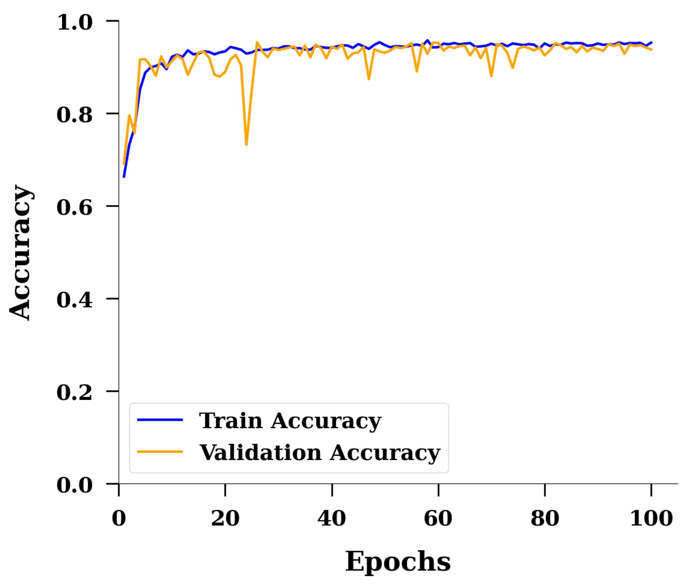
| % | 94.60 | 94.86 | 93.71 |
| MLP | Logistic Regression | Random Forest | SVM | |
|---|---|---|---|---|
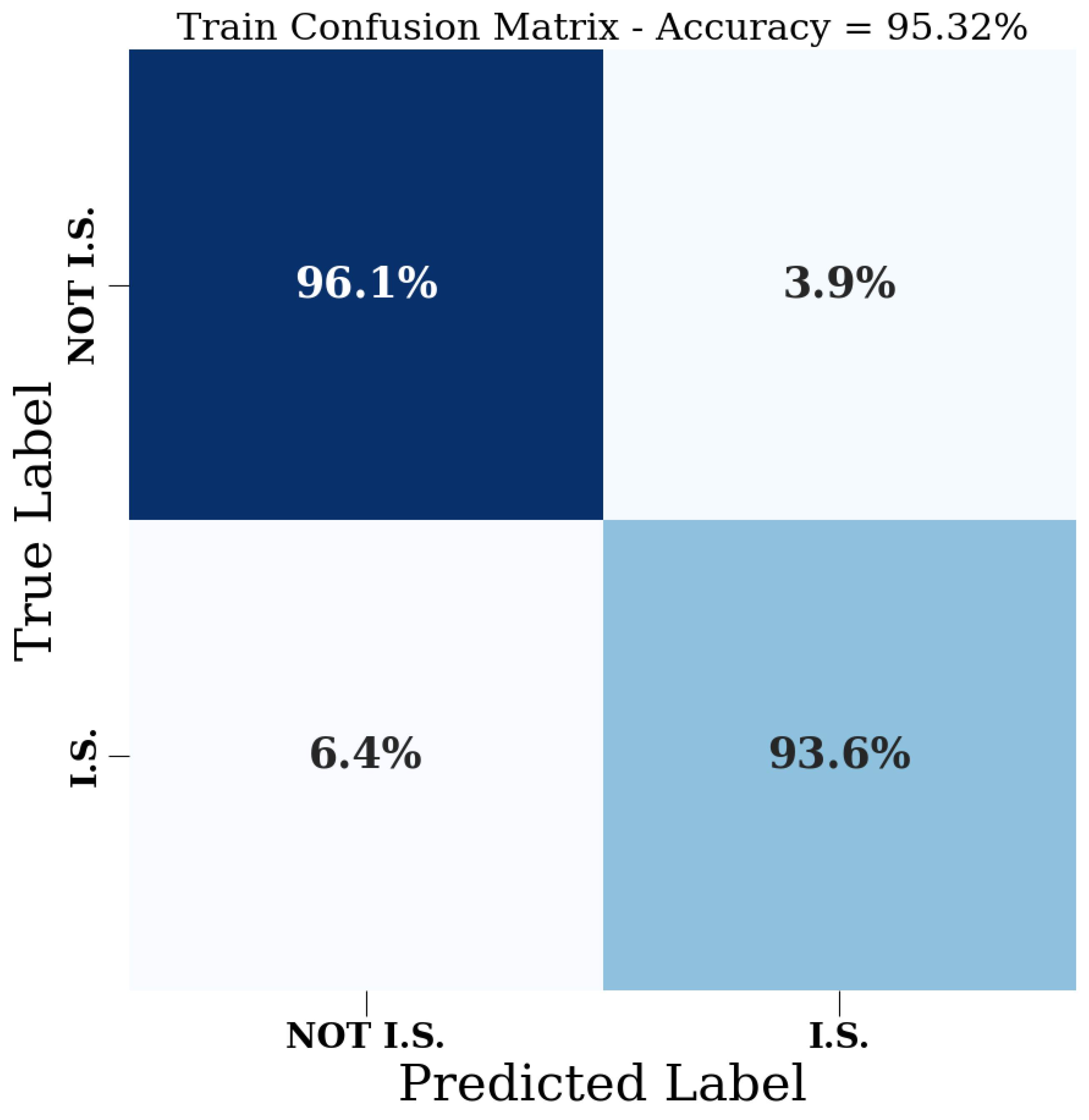
| Train. Accuracy | 95.32% | 70.07% | 100% | 75.15% |
| Val. Accuracy | 95.17% | 69.04% | 94.33% | 75.13% |
| Time | 27.99 s | 0.093 s | 0.66 s | 0.27 s |
Disclaimer/Publisher’s Note: The statements, opinions and data contained in all publications are solely those of the individual author(s) and contributor(s) and not of MDPI and/or the editor(s). MDPI and/or the editor(s) disclaim responsibility for any injury to people or property resulting from any ideas, methods, instructions or products referred to in the content. |
© 2024 by the authors. Licensee MDPI, Basel, Switzerland. This article is an open access article distributed under the terms and conditions of the Creative Commons Attribution (CC BY) license (https://creativecommons.org/licenses/by/4.0/).
Share and Cite
Tzimas, M.; Barbero, E.J. Imperfection Sensitivity Detection in Pultruded Columns Using Machine Learning and Synthetic Data. Buildings 2024, 14, 1128. https://doi.org/10.3390/buildings14041128
Tzimas M, Barbero EJ. Imperfection Sensitivity Detection in Pultruded Columns Using Machine Learning and Synthetic Data. Buildings. 2024; 14(4):1128. https://doi.org/10.3390/buildings14041128
Chicago/Turabian StyleTzimas, Michail, and Ever J. Barbero. 2024. "Imperfection Sensitivity Detection in Pultruded Columns Using Machine Learning and Synthetic Data" Buildings 14, no. 4: 1128. https://doi.org/10.3390/buildings14041128
APA StyleTzimas, M., & Barbero, E. J. (2024). Imperfection Sensitivity Detection in Pultruded Columns Using Machine Learning and Synthetic Data. Buildings, 14(4), 1128. https://doi.org/10.3390/buildings14041128