2.1. Case Study of a Pultruded Column: Finite Element Simulation Data Acquisition
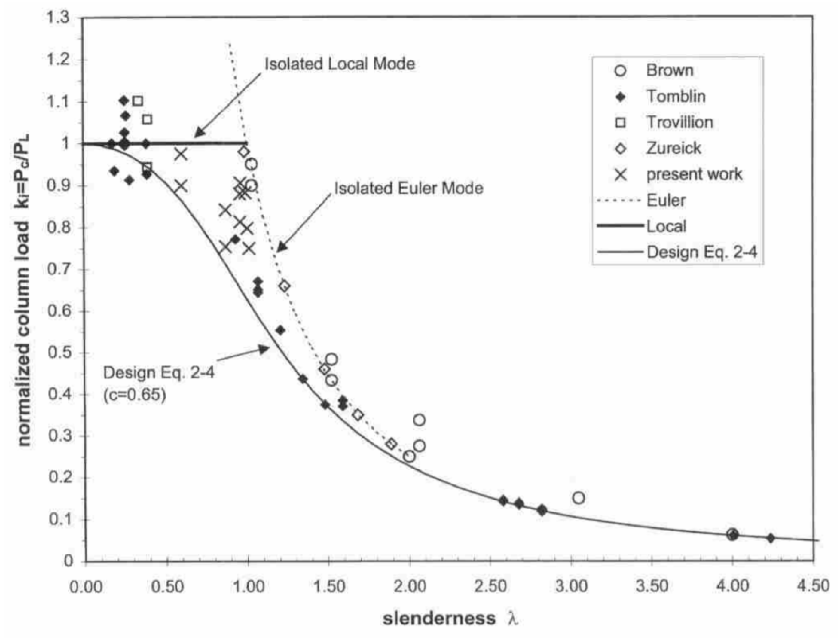
Pultruded structural shapes are thin-walled to take advantage of the high compressive strength of the fiber-reinforced composite material and to remediate the relatively low modulus of elasticity of the material. The flanges of the thin-walled section buckle first for stubby columns, but as the slenderness
increases, Euler buckling occurs [
5]. The local buckling load
is relatively constant, but the Euler buckling load,
, decreases sharply with the slenderness of the column. At the critical slenderness
, local and Euler loads coincide, i.e.,
[
6].
The slenderness of the column can be used in parametric studies. For perfect columns, there are two (isolated) observable modes, the local mode, for , , and the Euler mode, for , , where are material properties, L is the length, and K depends on the type of end-supports of the column.
Real columns are not perfect but rather have imperfections, which may be internal or external to the column. External imperfections include uneven axial lengths and eccentricities or non-uniformity of the applied load. Internal imperfections can be caused by damage or aging of the material. Therefore, for an imperfect column, the buckling load is less than the load predicted by either of the isolated modes described above, as shown in [
3,
6,
7] and multiple citations therein. Imperfection sensitivity can be reduced with a combination of manufacturing processes and targeted modeling as shown in ref. [
8].
In
Figure 1, both local and Euler modes are shown; however, for slenderness
between 0.7 and 1.2, multiple data points are observed to fall outside the isolated responses. Upon closer examination, these data points reveal the interaction between local and Euler modes. A design equation has been proposed that captures the behavior of the experimental observations across the spectrum of
[
3,
6].
To simulate imperfection-sensitive columns, Finite Element Analysis (FEA) is employed. Abaqus software is utilized to model columns with specified dimensions and material properties. Material properties are given in
Table 1 and
Table 2. Additional information regarding calculation and use of these material properties in Abaqus can be found in refs. [
10] and Ex. 3.11 and 4.4 in [
11].
Table 3 shows information regarding the FEA parameters used for meshing and boundary conditions. One end of the column has a symmetric boundary condition to reduce the overall length of the model. The cross-section, on the other end, has displacement constraints for rigid body motion, tied to a reference point. The load of the simulation is applied on the same reference point as a compressive force.
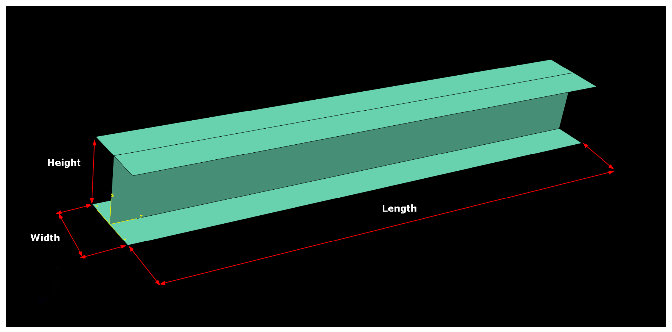
The perfect column is defined as a fiber-reinforced plastic (FRP) beam with a wide flange (WF) with dimensions
(WF 6 × 6). The width and height of the column are 6″, while the flange and web thickness are 3/8″ (9.525 mm). The length of the column is variable.
Figure 2 shows the relevant dimensions.
In practice, these columns are typically produced by pultrusion. The material properties reported in the tables were obtained analytically using the properties of the matrix (vinyl ester) and fibers (E-glass). Calculated material properties were validated experimentally [
12]. Furthermore, fiber density, architecture, and placement within the cross-sections were used in the calculations. The relevant matrix and fiber properties are widely available, while fiber architecture is proprietary to the manufacturer.
The critical length is found to be
= 2280 mm, and the critical load is
= 169.752 MPa. In order to generate multiple test cases, the slenderness
was varied from 0.5 to 1.5 (equivalent lengths
) to cover most of the cases that fall within the region of interest, as shown in
Figure 1.
Moreover, the chosen range of
allows for cases that are expected to produce mode interaction [
3], which is helpful in identifying whether columns are imperfection-sensitive (IS) or not. Imperfection sensitivity (IS) is identified by the presence of mode interaction, characterized by both lateral Euler deflection and flange deformation. Columns exhibiting only local, or only Euler modes are classified as non-imperfection-sensitive (NIS). Each mode has some expected responses, with local mode showing deformation on the flanges (wave patterns) and Euler mode showing lateral deflection of the whole column. Therefore, to correctly identify IS columns, both lateral Euler deflection and flange deformation must be observed.
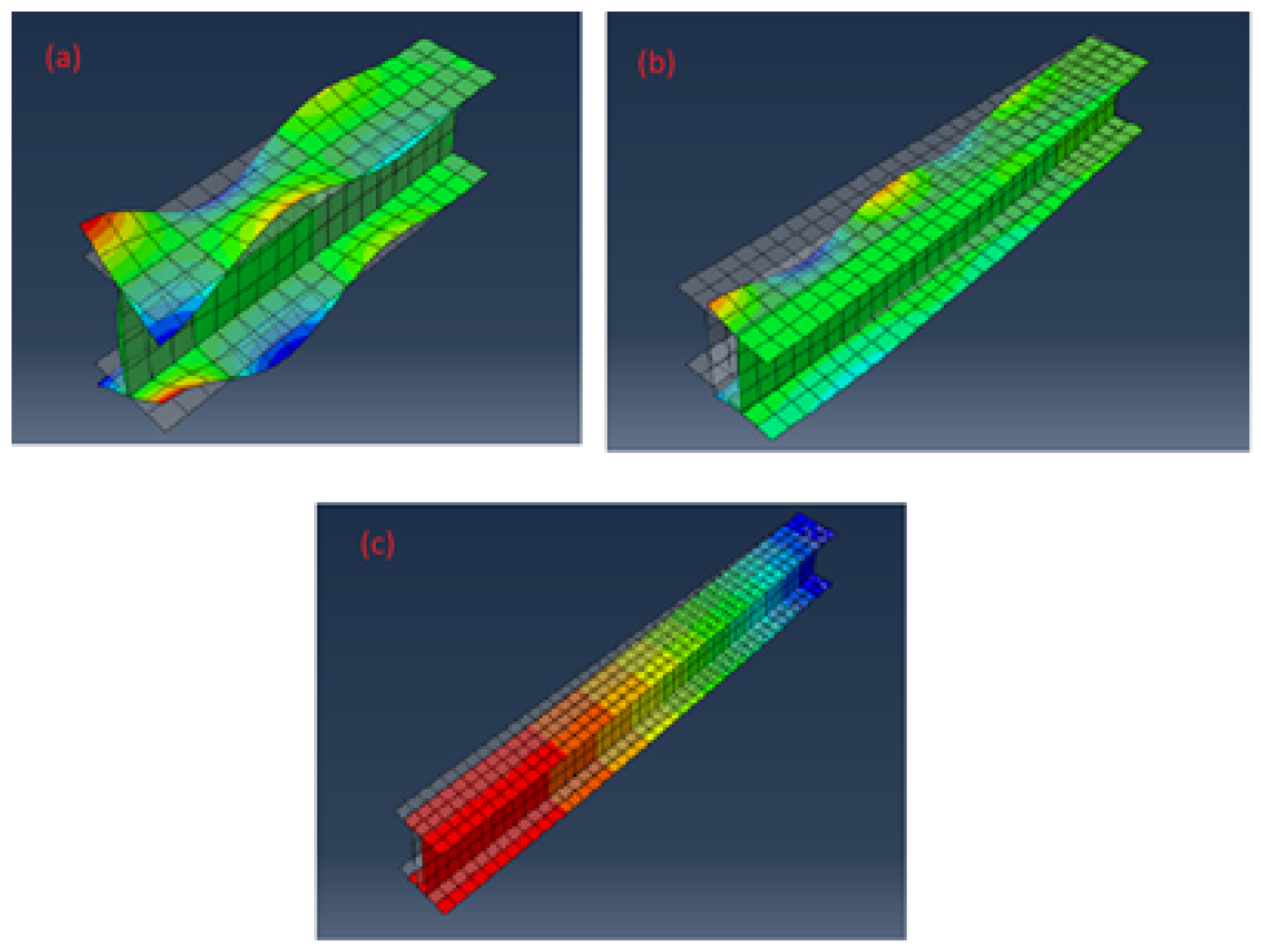
In FEA, the effects of imperfections can be modeled using perturbations in the geometry. In
Figure 3, we provide typical results of a column under buckling conditions. In
Figure 3a, we have flange deformation (wave undulations) for local mode, and in
Figure 3c we have lateral deflection, i.e., Euler mode. Based on the above discussion,
Figure 3a,c behave as NIS columns. On the other hand,
Figure 3b depicts an IS column, since there is an observable lateral deflection coupled with flange deformation.
In this work, synthetic data generation involved two phases: simulating perfect columns and introducing imperfections. ABAQUS performed buckling analysis to obtain eigenvalues and eigenmodes, representing limit loads and deformation shapes, respectively. Imperfections are introduced based on combinations of eigenmodes, simulating realistic conditions. The process for producing the synthetic data was fully automated and involved a single buckling analysis per length and multiple runs of each individual length when modeling imperfections on a second pass.
For instance, in
Figure 3c, depicting lateral deflection caused by the Euler mode, Abaqus illustrates the first eigenmode of the column, where the displacement is represented by the color scheme. Eigenmode 2 for the same column shows undulations and no lateral deflection. Thus, Abaqus essentially provides a Fourier transform of the leading components that make up all possible deformations of the column, since deformation in multiple axes and with different combinations of the Fourier modes is possible.
Imperfections were introduced based on combinations of two eigenmodes identified in the initial buckling simulations conducted for each length. The first eigenmode was always chosen to be the mode that produces lateral deflection (Euler). The second eigenmode was always chosen to be the mode that produces undulations on the flange, like
Figure 3a, with the smallest load. Imperfection values were set to geometric imperfections on the FEA mesh. Non-linear geometric analysis (NGA) in Abaqus is used to plot the load-deflection chart of the imperfect column.
Non-linear geometric analysis, utilizing the Riks method [
13] in ABAQUS, is the second step of the buckling analysis to simulate realistic conditions. After NGA is concluded, results similar to
Figure 3 can be found. Similar scenarios were observed in both experimental setups [
14] and in simulations [
9]. In this article, we conducted multiple Abaqus simulations, totaling N = 3750, aimed at detecting imperfection sensitivity through machine learning methods.
In this section, we discussed the methodology for acquiring data through Finite Element Analysis simulations of pultruded columns. The simulation setup includes modeling perfect columns and introducing imperfections to simulate real-world conditions. The parameters considered cover a range of scenarios, including mode interaction, to identify imperfection sensitivity. These simulations serve as the basis for generating synthetic data for subsequent analysis.
2.2. Machine Learning Model
Machine learning (ML) [
15] is a branch of Artificial Intelligence (AI) and is a rapidly growing field of study. ML involves algorithm development that allows computers to learn from data without explicit programming. ML is widely used in a variety of fields from everyday applications like image recognition [
16] to engineering applications such as microstructural characterization and prediction of mechanical response of crystalline materials [
17,
18]. Furthermore, ML has been used for failure mode identification and strength prediction in columns [
19,
20,
21,
22].
Applications of ML are generally separated into three types: supervised, unsupervised, and reinforcement learning [
23]. In this work, we focus on supervised learning, where algorithms learn from labeled data to make predictions on unseen data. Neural networks (NNs) [
24], inspired by the human brain’s structure, are commonly used for supervised learning tasks. Specifically, we employed deep neural networks [
25], or multilayer perceptrons (MLPs), which consist of input, hidden, and output layers.
Neural or deep neural networks are specific algorithms that are modeled after human brain synapses, exploring possible linear permutations and connections between data points in a set. In neural networks, there is an input layer for the features of the dataset, followed by a layer of hidden units and a final output layer. Deep neural networks operate on the same principle but with multiple hidden layers between input and output. The input and hidden layers consist of multiple nodes, upon which mathematical operations are performed. Based on the result of the operations and whether that result can be “activated” via an activation function, or not, the nodes can be discarded, or the result can move to the next layer. When the information only travels forward (i.e., from the input layer to the hidden layers and then to the output layer), the networks are considered feedforward neural networks. When there are at least three layers (including input and output) in a feedforward NN, it is considered a multilayer perceptron (MLP).
As the process moves forward and multiple combinations are tested, the network reaches the output layer, which normally consists of 2 nodes in binary format (0 or 1) with a probabilistic outcome. For example, if in the final hidden layer the permutations and activation function give a result of 0.1, the result is binarized as (0.9, 0.1) for the output layer, meaning that there would be a 90% chance that the particular data point would belong to group 0. Once multiple data points have gone through the network (known as a batch), the next batch follows until all batches (or training data) have gone through (known as an epoch).
During a forward pass of a batch, the neural nodes are trained to learn useful permutations by applying biases and weights. At the end of the training of the batch, the predicted outcomes in the output layer are tested against the known outputs to define a loss function [
26].
The loss function is propagated backwards through the layers to optimize the weights in each node of each hidden layer. With the end of training of an ML model (i.e., after all epochs have finished), the weights are supposed to be optimized and can be further validated and tested. If the validation and testing phases give results with similar accuracy to those of the training step, the ML model can be deployed (i.e., the optimized weights can be applied to data with similar features). At this point, the ML algorithm would be ready to be deployed in the field, where it would be capable of predicting, for example, the failure load reduction for a given set of deformations measured in the field in real time.
In this work, we employed deep neural networks i.e., multilayer perceptrons (MLPs) with four hidden layers which were trained on a set of 2625 columns with 151 identifying features and then validated on a set of 1125 columns with the same number of features.
We employed the Tensorflow Python library [
27]. The input layer includes the whole training dataset, which is then passed through the hidden layers. Each hidden layer progressively shortens the number of available neurons (nodes) until the binary output unit is reached. Each layer, except the output, uses the Rectified Linear Unit activation function [
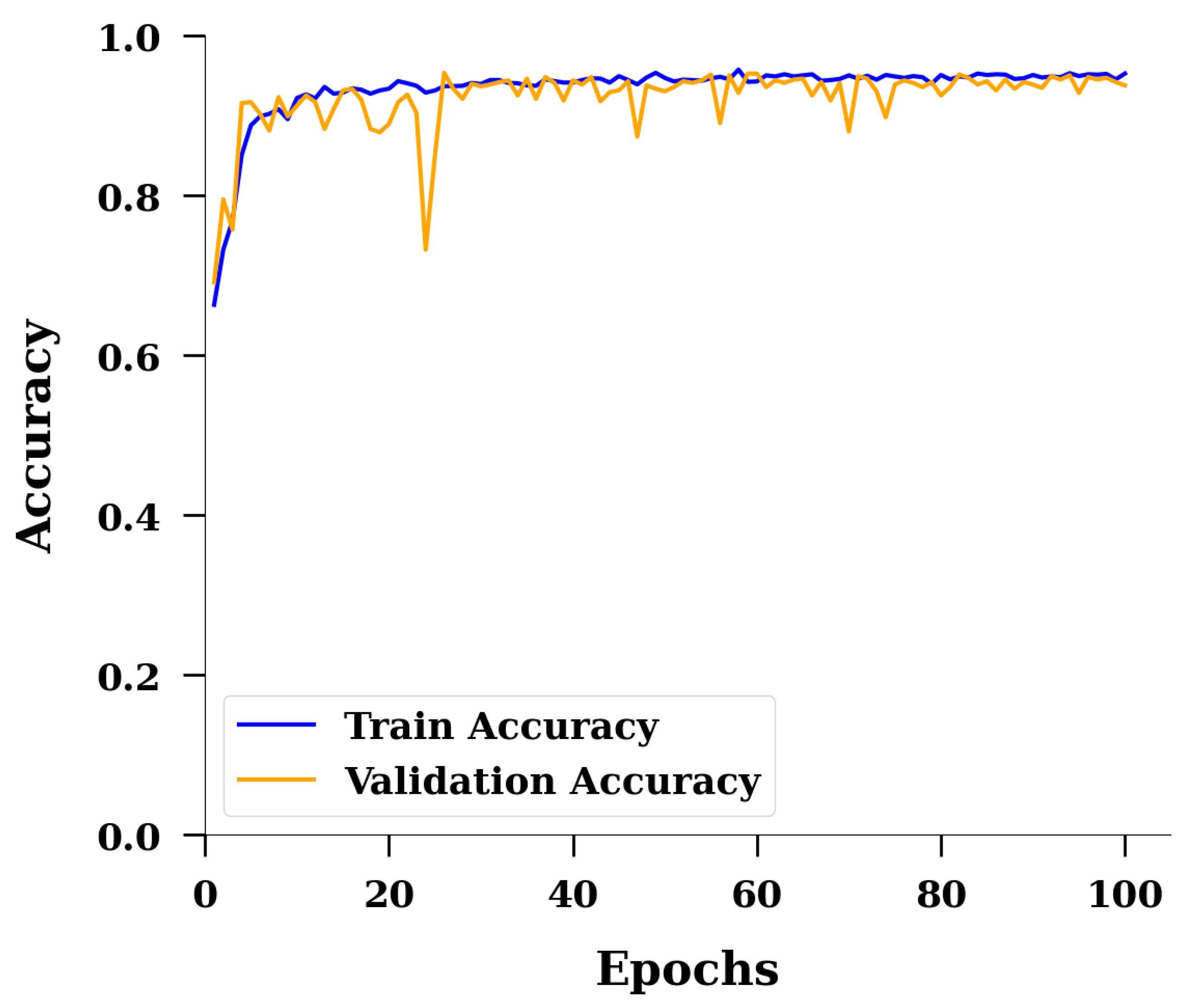
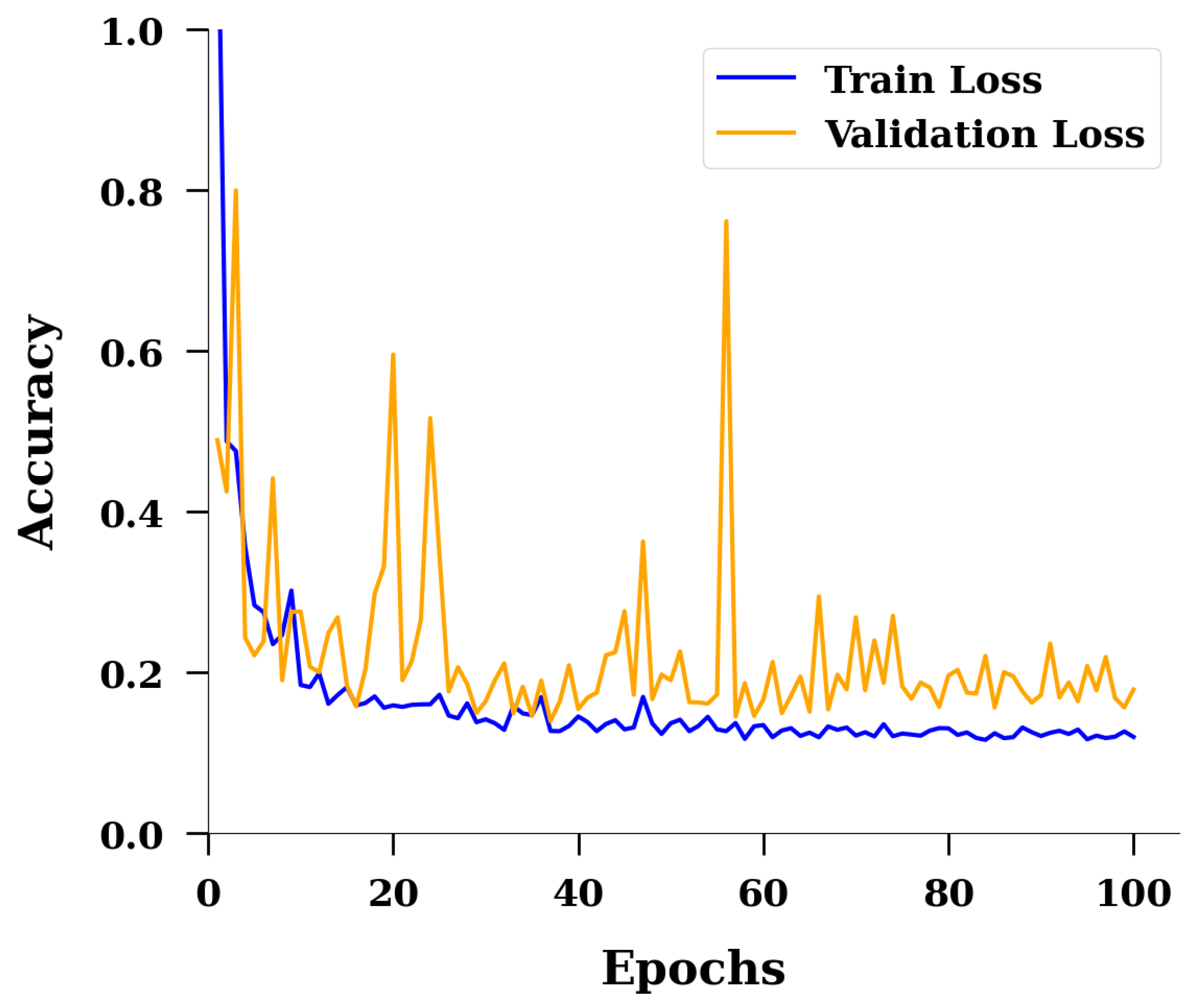
28] in each node to assess whether the neuron is important to the training, or not. The output layer employs the softmax activation function in each of the two nodes to convert the value to a probability distribution of the two possible outcomes. The training lasted 100 epochs, with a batch size of 100 columns in training.
2.3. Finite Element Simulations and Feature Selection
In a supervised ML problem, both the inputs and outputs need to be known. Therefore, prior to our ML training, we needed to determine which columns are considered imperfection-sensitive based on our Abaqus simulations. To do so, the following assumptions were made:
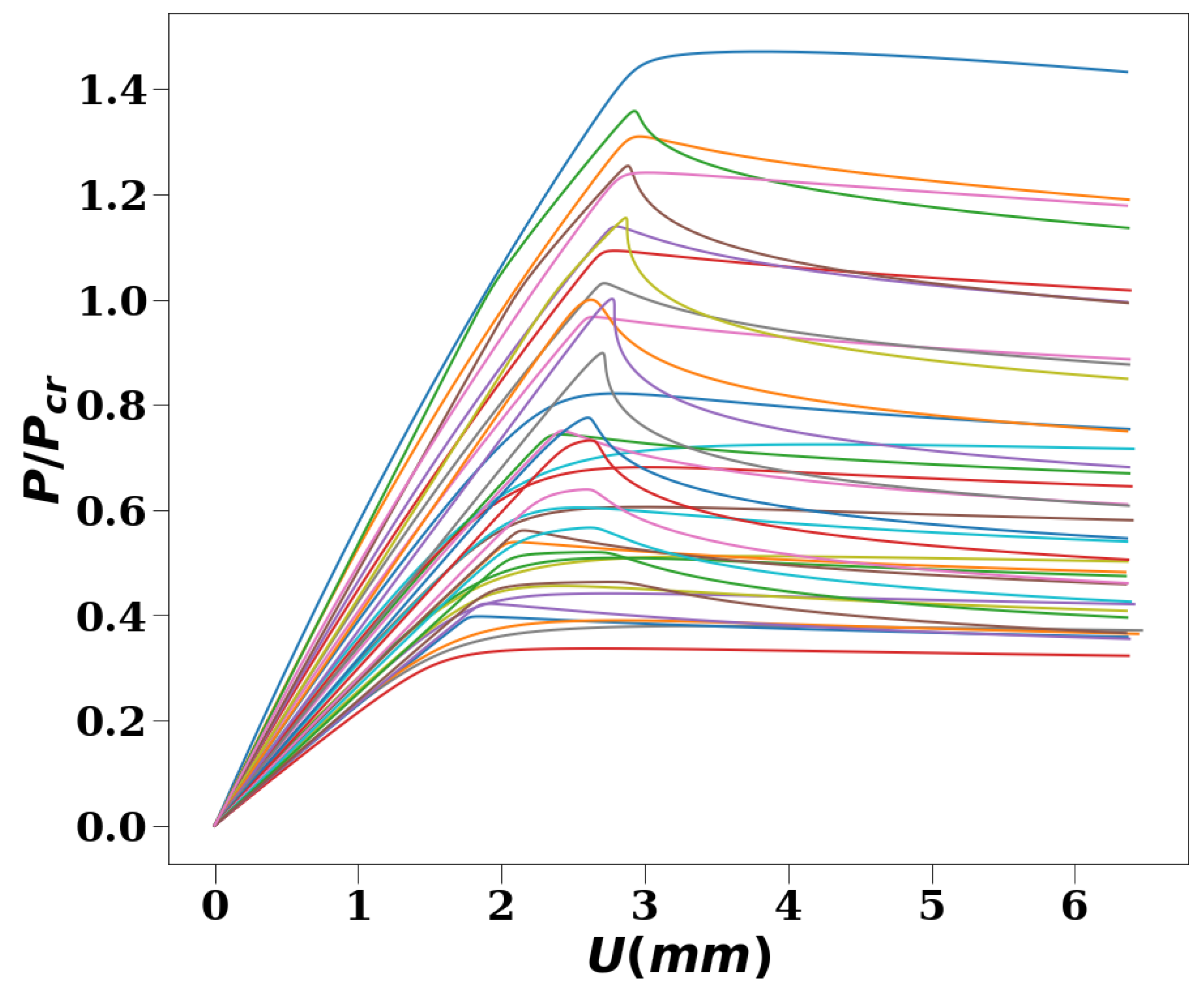
This means that if the peak load (
) found in NGA is less than the critical load (
) and the final load in the simulation (
) is at least 15% less than the peak load, and furthermore the final load occurs at a higher displacement (
) than that of the peak load (
), then the column is imperfection-sensitive, as shown in
Figure 4. Some columns may satisfy some parts of the equation and, in particular, the first part. However, if there is no observable load drop, the columns are not necessarily imperfection-sensitive but may just be following the Euler or local modes.
Lateral deflection in
Figure 4 is found from a reference point (RP) in the ABAQUS discretization, and extracted with the following ABAQUS Script:
xyList = xyPlot.xyDataListFromField(
odb=odb, outputPosition=NODAL, variable=((
’CF’, NODAL), (’U’, NODAL), ), nodeSets=(’SET-RP’, ))
x0 = session.xyDataObjects[’CF:CF3 PI: ASSEMBLY N: 1’]
x1 = session.xyDataObjects[’U:U3 PI: ASSEMBLY N: 1’]
The script implements the Riks method, controlling both the load
P and the
deflection of the RP. The RP is located at the point of load application.
Figure 4 is made from “force-stroke” curves for every 100th sample column.
Once IS samples are identified, the next step is to identify which inputs can be used to train our algorithm. The inputs need to be experimentally tractable so that the proposed method applies to field data as well. Moreover, it is preferred that instrumentation to collect filed data is inexpensive; while ABAQUS gives us great latitude in choosing inputs to train our algorithm, our options for experimental data are rather limited. Specifically, we cannot use the peak load or any load close to the service load because we would need to experimentally measure deformations when the column has failed or is close to failure. Thus, our goal is to train our ML algorithm with data collected for loads no larger than 30% of the service load for any given column. Furthermore, it must be noted that we can use any observable deformations that occur for smaller loads, both for training and for in situ monitoring of the deployed SHM system. The length of the column is also an observable variable.
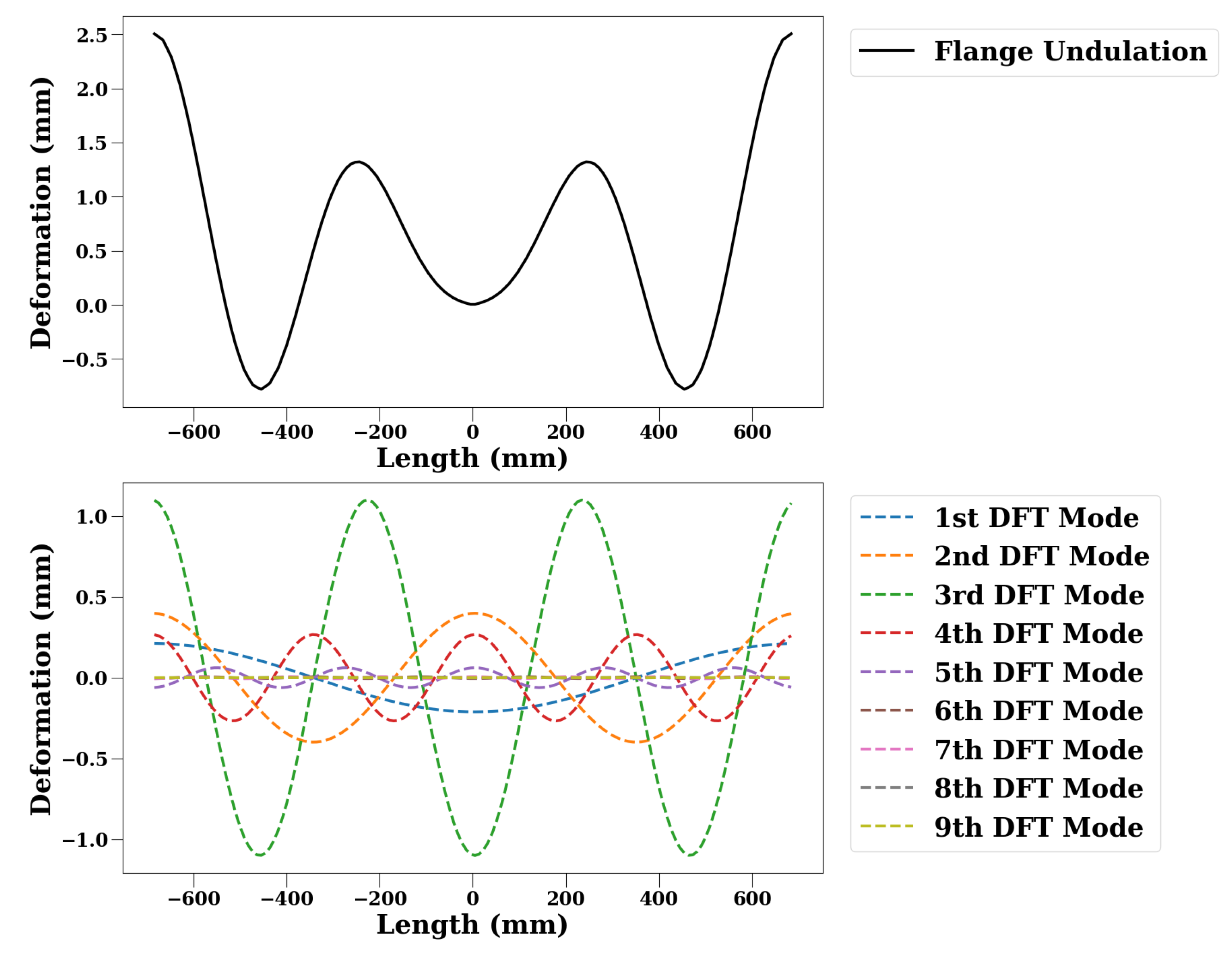
As imperfection sensitivity is the combination of local and Euler modes, and as local modes manifest themselves with undulations on the flanges of columns, we can use the undulations as our experimentally observable features. Undulations in local modes can be visually observed in loads as low as 20–30% of service loads, as corroborated by simulation presented herein and by experimental observations [
14]; thus, they are prime candidates for use as inputs in our ML pipeline. Specifically, we apply a Discrete Fourier transform (DFT) using a Fast Fourier Transform algorithm (FFT) [
29] on the undulations, since they present a sinusoidal form (see
Figure 5).
DFT was performed with the Python library NumPy [
30]. The python algorithm that performs DFT requires a one-dimensional signal (input) over a specified domain. We chose the domain to be the length of the column, and our signal is the wave undulation. We specified an arbitrary number (10) of sine frequency components that may comprise our signal, and we determined which of these components contributes the most (leading frequency component). Once the leading frequency component was found, an inverse Fourier computation allowed us to transform the leading frequency component back to a one-dimensional signal. In summary, we disassembled the signal into multiple contributing signals of various frequencies then kept the largest contributor for our purposes. This (largest) isolated mode is the leading factor of deformation on the flange.
We can extract the nodal displacements in two ways. For this study, we extracted them from Abaqus simulation. However, in an experimental or field implementation setting, we would extract them from a laser deflectometer or similar instrumentation that can be used to monitor the flange displacements. In any case, extraction of nodal displacements is always followed by a DFT to isolate the leading modes.
In this work, Abaqus nodal displacements at 30% of service load were used to create the undulations. DFT and subsequent inverse DFT were used to extract the leading sinusoidal form of the nodal displacement. The displacement of each node (150 in total) was used as an input feature in our ML pipeline, and the length of the column led to a total of 151 experimentally observable features that were used to train our ML model to recognize IS columns.
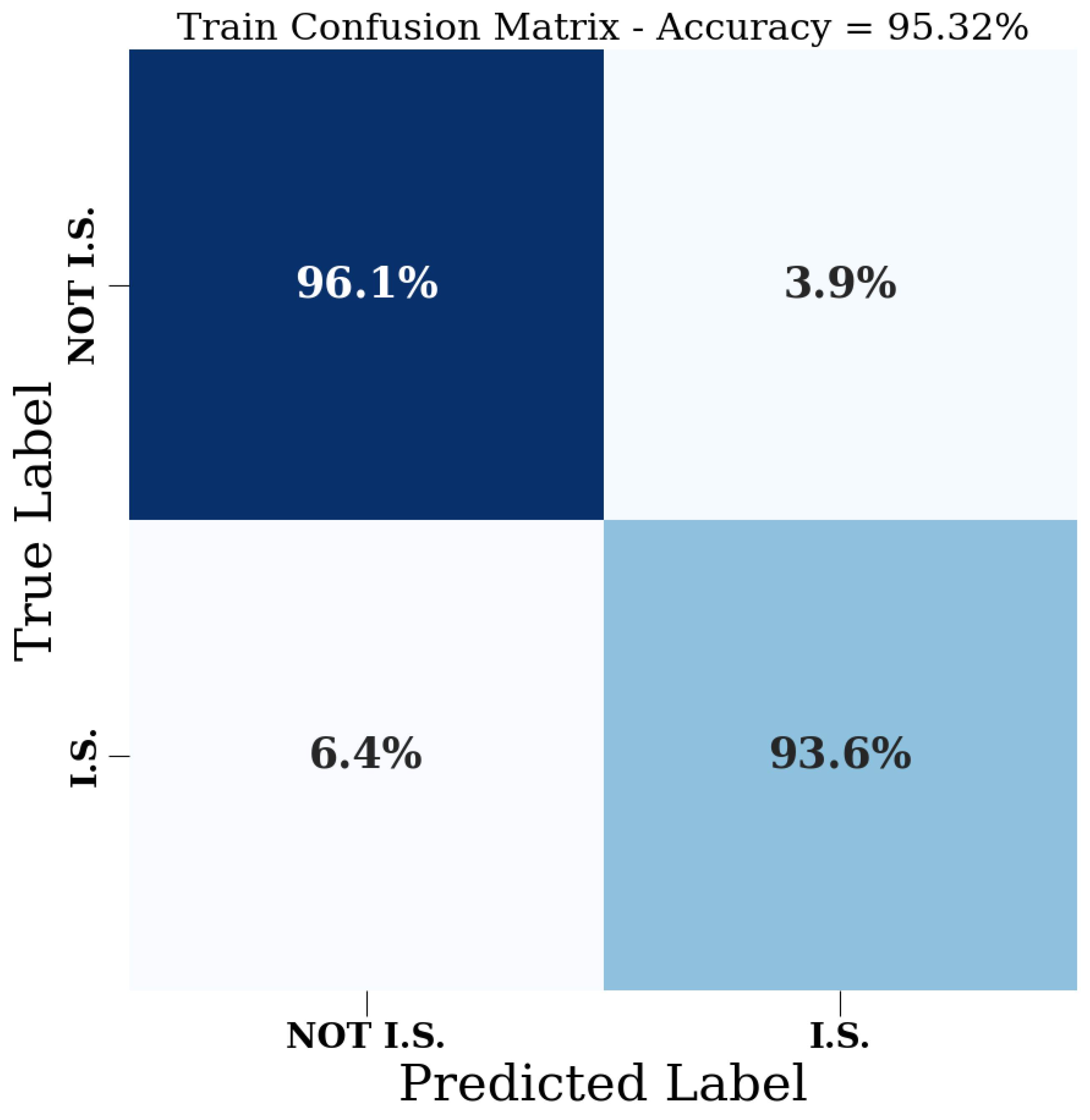
In total, our deep neural network comprises 2750 columns, which have 151 features to describe whether they are IS or not. All features are used as an initial input and are fed forward to our four hidden units of decreasing nodes for a total of 100 epochs to maximize accuracy and efficiency. The output must be cast as a binary classification of 0 and 1, where 0 indicates a NIS column and 1 indicates an IS column. The model parameters at the final epoch are used to evaluate the test data (1125 columns) which has the same number of input features and is not used for training but set aside for testing the accuracy of the trained NN. To reduce the model complexity and the overall number of training parameters, it may be possible to use weight quantization or network pruning techniques [
31].


