Multiaxial Fatigue Damage Analysis of Steel–Concrete Composite Beam Based on the Smith–Watson–Topper Parameter

Abstract

The fatigue performance of steel–concrete composite beams is crucial for ensuring structural safety. To account for the member’s multiaxial stress state, this study employed the critical surface method, using fatigue damage parameters as an evaluation index for assessing fatigue performance. Static and fatigue performance tests on steel–concrete beams were conducted to identify failure characteristics, which informed the development of a finite element model that incorporates concrete damage. Using the SWT model, the most unfavorable loading parameters were determined by analyzing critical paths on the test beams, providing a basis for predicting how initial defects impact fatigue performance. The impact of initial defects on the fatigue performance of the composite beam is assessed using this criterion. The results indicate that the discrepancy between the actual and predicted load capacities of the test beam is within 5%, and cyclic loading significantly affects the test beam’s mechanical properties, resulting in a 27% reduction in load capacity and a 48% increase in deflection after 2 million cycles. Finite element modeling reveals that components experience multiaxial stress, with test beam mechanical property changes aligning with predicted fatigue damage parameters, confirming the reliability of using these parameters as a criterion. As the strength of the composite beams diminished due to pore defects, the fatigue damage parameter escalated, increasing the likelihood of crack formation. However, once the concrete’s strength fell to a level where the pegs were insufficiently constrained, the structural damage pattern shifted, and the fatigue damage parameter subsequently decreased.

1. Introduction

Steel–concrete composite structures integrate the advantages of both steel and concrete and are widely used in the construction of buildings and bridges due to their superior performance and convenience in construction [1]. The excellent performance of steel–concrete composite structures makes them of significant research interest, thus studies in this field have been thriving for a long time. Innovations are continually made in materials [2,3], and various excellent application structures appear in areas such as large-span bridges and urban overpasses [4,5].

The widespread use of steel–concrete composite structures necessitates closer scrutiny of member defects and the decline in stress performance, among which the fatigue performance of shear connectors is a primary concern [6]. Despite numerous fatigue tests conducted by scholars worldwide on composite beams, the internal damage within composite beams remains challenging to detect. Consequently, this paper employs a numerical analysis to evaluate the performance of composite beams, utilizing practical engineering cases and theoretical frameworks [7]. Conventional methods often employ S-N curves to assess the relationship between nominal shear stress amplitude and fatigue life cycles in shear connectors, utilizing experimental data for fitting. Under uniaxial stress, S-N curves can effectively evaluate fatigue due to the straightforward nature of the loading history. However, in numerous practical applications, multiaxial and non-proportional loading conditions are encountered, making S-N curve-based fatigue predictions insufficient. Furthermore, most S-N curve models in the study are tailored to fit specific test data, lacking a universal model for precise predictions [8]. Additionally, the S-N curve method fails to accurately predict fatigue life when accounting for the impact of initial defects, potentially resulting in an overestimated infinite fatigue life. Moreover, the method demands extensive experimental data to assess fatigue life under variable amplitude loading, which can be prohibitively expensive [9]. Thus, traditional evaluation methods may be limited when assessing the fatigue performance of shear connectors across diverse types and application scenarios.

The stress state at a point within a structure can be characterized by a two-dimensional tensor that includes three normal and three shear components, with any directional change during the actual stressing process altering the magnitude of each stress component. Experimental research by scholars such as Xiang et al. has shown that bolts, acting as shear connectors, not only bear shear in the shear region but also induce significant compressive stress on the hole wall and longitudinal and transverse tensile stresses within the concrete. Consequently, in practical engineering applications, shear connectors are subjected to not only shear stress but also complex multiaxial stress conditions [10,11]. Currently, the primary methods for assessing multiaxial fatigue life include the nominal stress method, the local strain method, and the critical plane method, with varying applicability across different cases. The Smith–Watson–Topper (SWT) model has been refined through numerous modifications and derivations by scholars [12]. Scholars Li [13] and Branco [14] confirmed the SWT model’s accurate predictions for shear connectors by comparing it with the Topper criterion and evaluating the predictive accuracy of the SWT, CM, and TSED models. Steel–concrete composite structures, as a whole, have the concrete as one of their main components, which is a typical non-homogeneous and porous material, influenced by various factors, including construction methods, curing conditions, and environmental humidity. This results in the concrete inevitably having initial pore defects; these initial defects, along with other quality issues, are among the primary factors affecting the mechanical properties and durability of concrete. The interaction between the components places the composite beam under a complex multiaxial stress state. In most cases, the fatigue characteristics of the exterior of the composite components can be intuitively deduced. However, fatigue damage within the components is challenging to predict; therefore, these issues necessitate further in-depth study.

Building on the research described above, this study conducted fatigue tests to discuss the effects of relative slippage, strain outcomes, and changes in deflection on the components. Based on these findings, a finite element analysis model was established. Utilizing the damage critical plane method with the Smith–Watson–Topper (SWT) parameter as the evaluation criterion, the fatigue states of the composite beam’s shear connectors and the steel longitudinal beam’s welded details were assessed. Furthermore, a parametric analysis of the fatigue state of the welded details under the impact of initial concrete porosity defects was also performed.

2. Experimental Program

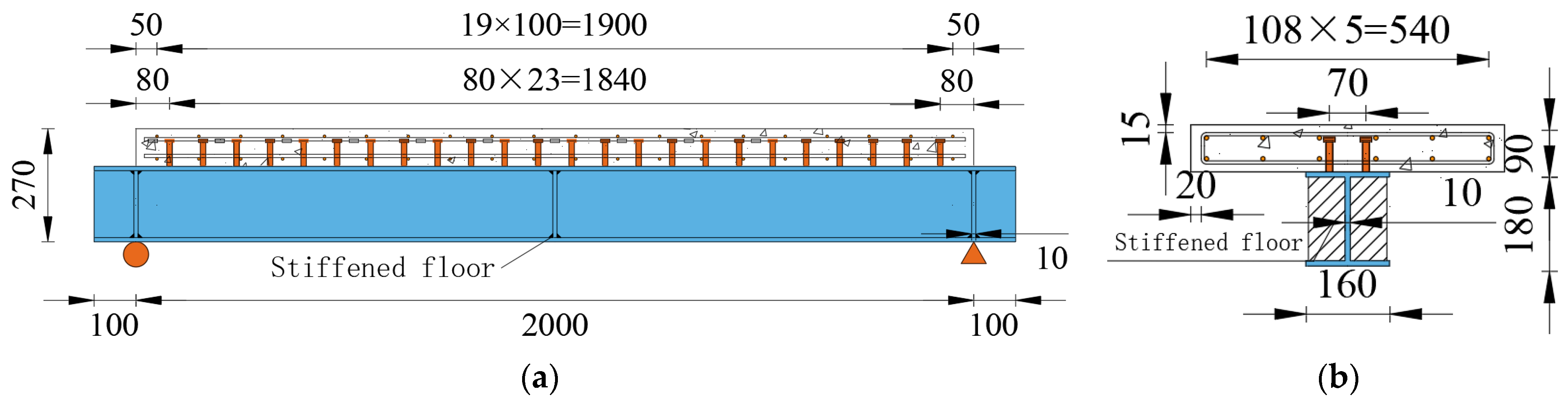
2.1. Test Specimen Geometry and Material Properties

The experimental model is constructed as shown in Figure 1. The total length of the experimental beam is 2.2 m, with a calculated span of 2 m, divided into two pieces: one for static tests and the other for fatigue tests. Both beams share identical geometric parameters, where the concrete slab uses C40 concrete and the steel is Q235, welded into an I-shaped steel beam according to standards. Specific parameters are available in

Table 1. Material parameters.

Component	Material	Size Settings (mm)
Longitudinal rebar	HPB300	$\phi$8@108
Transverse rebar	HPB300	$\phi$6@100
Steel plate	Q235	2200 × 160 × 10
Concrete slab	C40	2000 × 600 × 100
Stud connectors	ML-15	$\phi$13@80

. Vertical stiffeners are arranged at the supports of the steel beam and at the mid-span to enhance the stability of the steel beam at these specific local positions. The experimental beams are designed with fully shear-resistant connections using ML-15 type 13 studs, arranged in double rows with a transverse spacing of 70 mm and a longitudinal spacing of 80 mm, totaling 48 studs.

2.2. Load Bearing-Capacity Calculation

To determine the appropriate loading method, this paper preliminarily calculates the plastic bearing capacity of the test beam. Several basic assumptions are made in this process: Firstly, the stud connectors ensure a tight connection between the concrete flanges and the steel beam, thus fully utilizing their bending resistance. Secondly, it is assumed that the concrete below the plastic neutral axis has cracked and does not participate in load bearing. Lastly, the concrete under compression and the steel beam under tension and compression have both entered the plastic state, with their stress distribution appearing rectangular across the cross-section [15].

To begin, calculate the relationship between the force in the steel beam, A_sf_y, and the force in the concrete slab, b_effh_df_ck, to determine the type of section. Based on the material performance test results, the axial compressive strength standard value, f_ck, of the concrete is set at 30.6 MPa, and the yield strength, f_y, of the steel beam is set at 345 MPa. If the calculation shows that A_sf_y is greater than b_effh_df_ck, the section is then calculated as a Type II section (Figure 2).

Let the compressive area of the steel beam be A_sc; then, the tensile area of the steel beam, A_st, is the difference between A_s and A_sc. According to the section force balance condition which equals zero, Equation (1) can be derived as follows:

$$A_s{f}_y+b_{eff}{h}_d{f}_{ck}=(A_s-A_{sc})f_y$$

(1)

where A_s represents the cross-sectional area of the steel beam, b_eff represents the effective width of the concrete slab, and h_d represents the height of the concrete slab.

Based on Equation (1), it is calculated that A_sc is less than the force-bearing area of the upper flange of the steel beam, b_sut, indicating that the plastic neutral axis is located within the upper flange of the steel beam. After confirming the balance position, Equation (2) is used to calculate that the bending moment of the component is 222.4 kN.

$$M_u=f_y[A_s(h-y_{sb}-\frac{h_d}{2})-b_{su}(x-h_d)(x-\frac{h_d}{2})]$$

(2)

Finally, let P denote the load at the mid-span loading position of the test beam. When the shear effect is at its maximum, based on the balance equation, the estimated load on the test beam is calculated to be 444.8 kN.

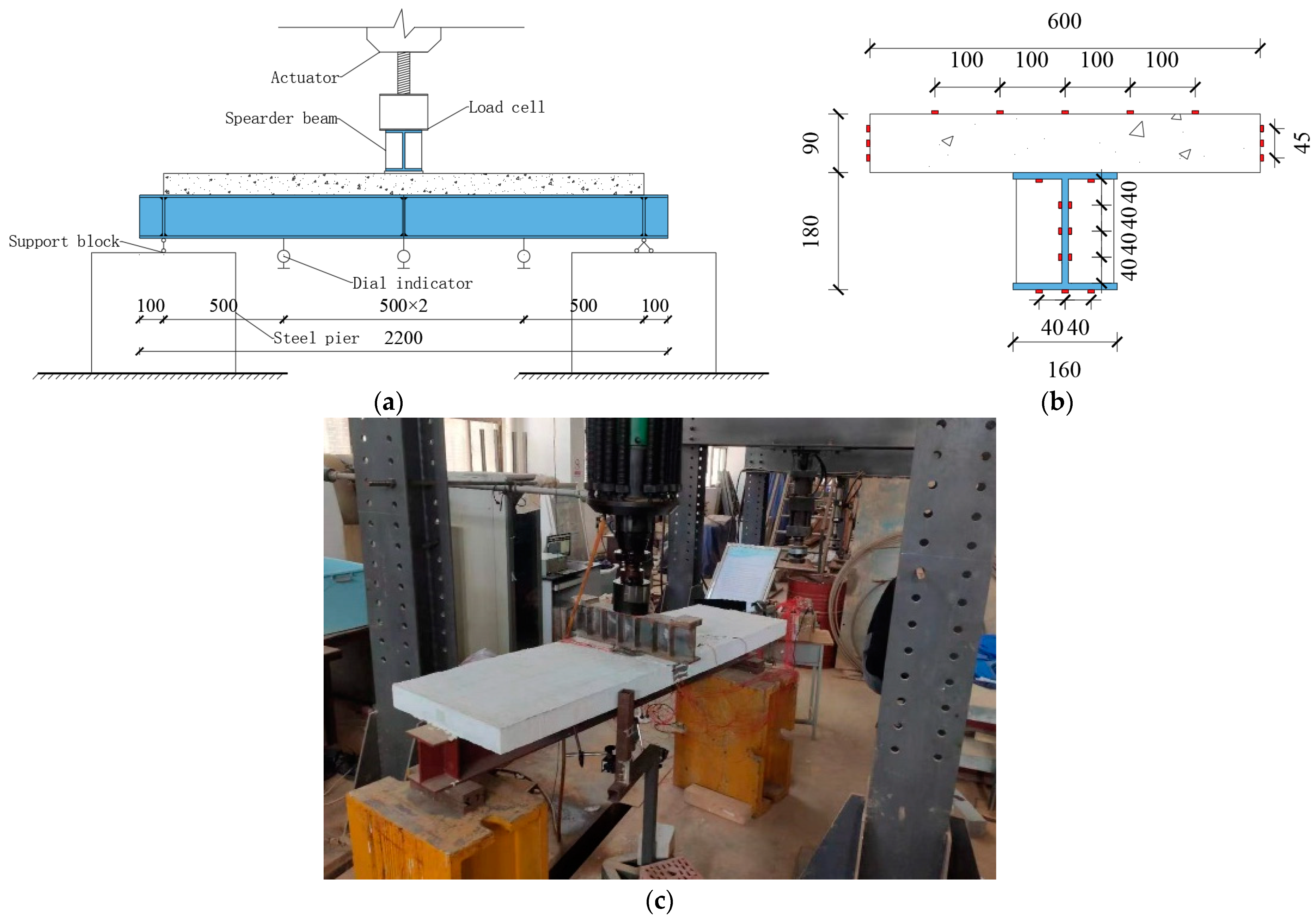
2.3. Loading and Measurement Setup

To maximize the shear effect, all test beams are designed to be simply supported and are subject to single-point loading at mid-span. A steel plate is placed at the loading point on the concrete slab to ensure even distribution of forces on the test beam. Before loading, the load center is confirmed to be at the midpoint of the test beam using a pendulum hammer, and the supports are adjusted by methods such as spreading fine sand to ensure even force distribution across the beam. Before actual loading, a pre-load operation is conducted during static tests to eliminate factors such as residual adhesion, which might affect loading. During the pre-loading phase, the load increments are set between 0.2 and 0.4 times the elastic limit load, and after reaching the target load, it is completely released.

To further understand the elastic–plastic behavior of the test beam at different stages, a stepwise incremental loading method is used, with each increment being 20 kN and the loading rate controlled at 2 min per increment. When the load reaches the limit of the elastic stage, the loading is switched to displacement control at a rate of 0.25 mm/min, and this process continues until component failure. Each loading stage is maintained for 2 min to collect data on load values, displacement at various points, and strain readings (see Figure 3).

Similar pre-loading is performed before the cyclic load testing. During the actual loading phase, the cyclic loading is paused when the component has undergone 500,000, 1,000,000, and 1,500,000 cycles to perform a static data collection of the elastic stage. The collected data represent the bearing capacity performance after the nth cycle, culminating in static failure. The upper and lower fatigue loading limits are based on a bearing capacity degradation model and range from 0.35 P_u to 0.6 P_u (where P_u is the ultimate load). The fatigue load control waveform is sinusoidal, and the loading frequency is 4 Hz.

3. Test Results and Analysis

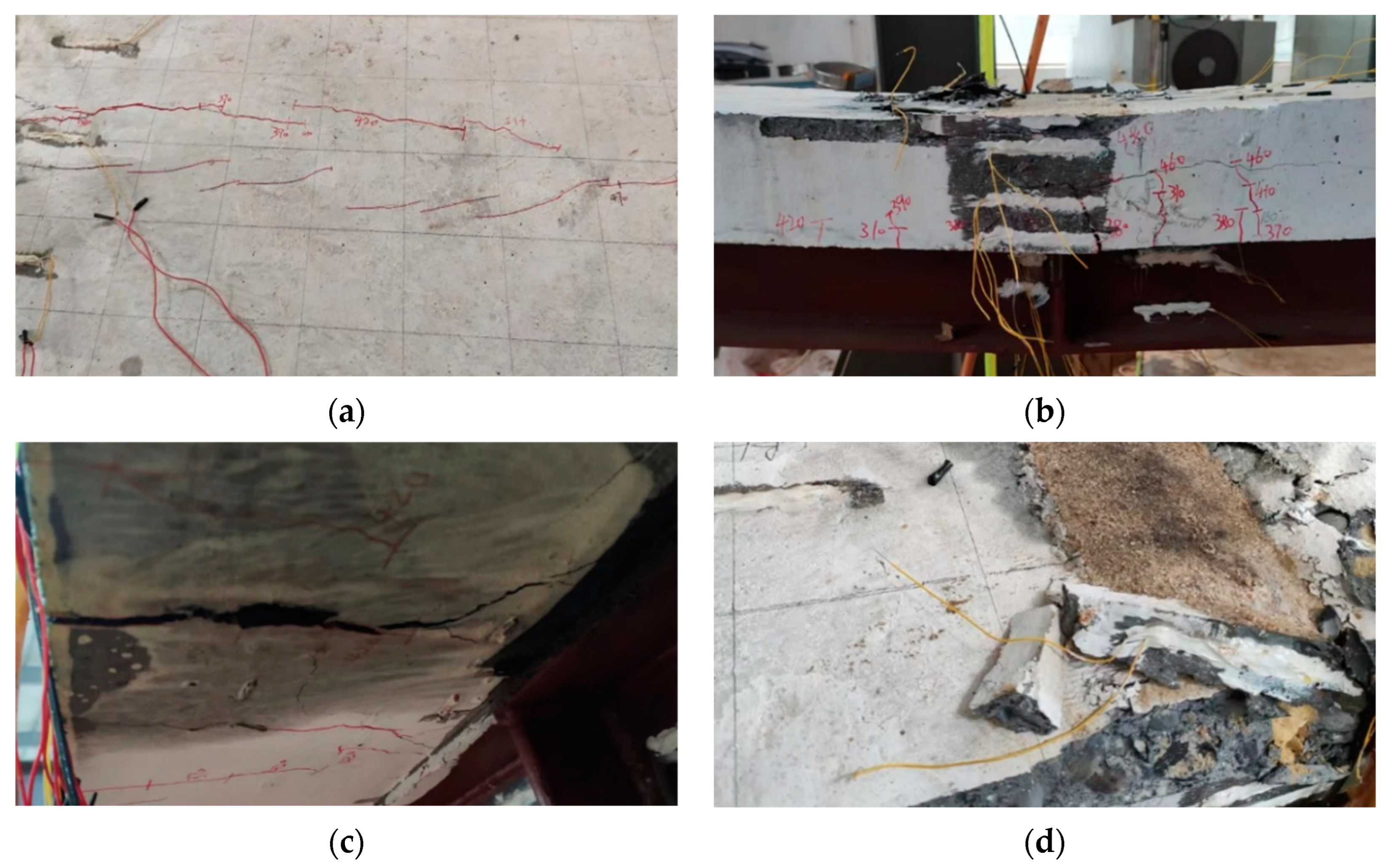
3.1. Failure Process

At the initial stages of load application, the test beam is in the elastic phase, with displacement and strain showing a linear relationship. When loaded to 0.4 P_u, stresses concentrate in the concrete slab due to the direct application of loads, and transverse cracks appear in the central loading area of the concrete slab’s top surface and gradually expand as the test force increases. At 0.7 P_u, the test beam enters the yielding phase, the concrete slab experiences significant bending moments at mid-span, and interfacial slip between the steel reinforcement and the concrete causes localized stress concentrations. Longitudinal cracks appear near the mid-span on the underside of the concrete slab, and these extend upwards as the load increases, eventually enveloping the entire section. After the load reaches 0.85 P_u, diagonal cracks appear on both sides of the concrete loading point, accompanied by spalling of the concrete, and the displacement corresponding to the same load increment significantly increases. At this point, the loading is nearing its end, the concrete strength is at its limit, and the bond between the concrete and the steel beam is inadequate. Afterwards, the growth rate and number of cracks on the concrete slab rapidly increase, continually extending and interconnecting. Approaching the ultimate load, the concrete flange at the loading point is crushed, with a large amount of concrete spalling and significant yielding deformation of the steel beam. The experimental destruction phenomenon is shown in Figure 4.

After 500,000 load cycles, minor cracks appear at the connection between the steel beam and the concrete slab, with the overall load-bearing capacity of the test beam remaining essentially consistent with that before cycling. As the number of load cycles increases to between 1,000,000 and 1,300,000, horizontal expansion of surface cracks on the concrete slab and longitudinal cracks at the mid-span occur, slightly reducing the load-bearing capacity. After 2,000,000 load cycles, the steel beam exhibits slight bending deformation, and transverse cracks extend to a quarter of the beam’s span. Under cyclic loading, fatigue damage, such as cracking, reduction in shear resistance, reduction in bonding properties, and reduction in structural stiffness, was observed in the combined beams. Subsequently, under static loading to 0.5 P_u, the crack at the lower edge of the concrete flange at mid-span spread to form a through crack, and a sudden change occurred in the vertical displacement at the center of the steel beam. When loaded to 0.6 P_u, the transverse cracks rapidly expanded to the supports. Finally, when loaded to 0.85 P_u, dense brittle sounds occurred inside the concrete, and as the load approached the ultimate load, the concrete near the loading beam fractured, and a significant amount of concrete spalled, leading to the destruction of the test beam. Experimental destruction phenomena are similar, but they occur earlier.

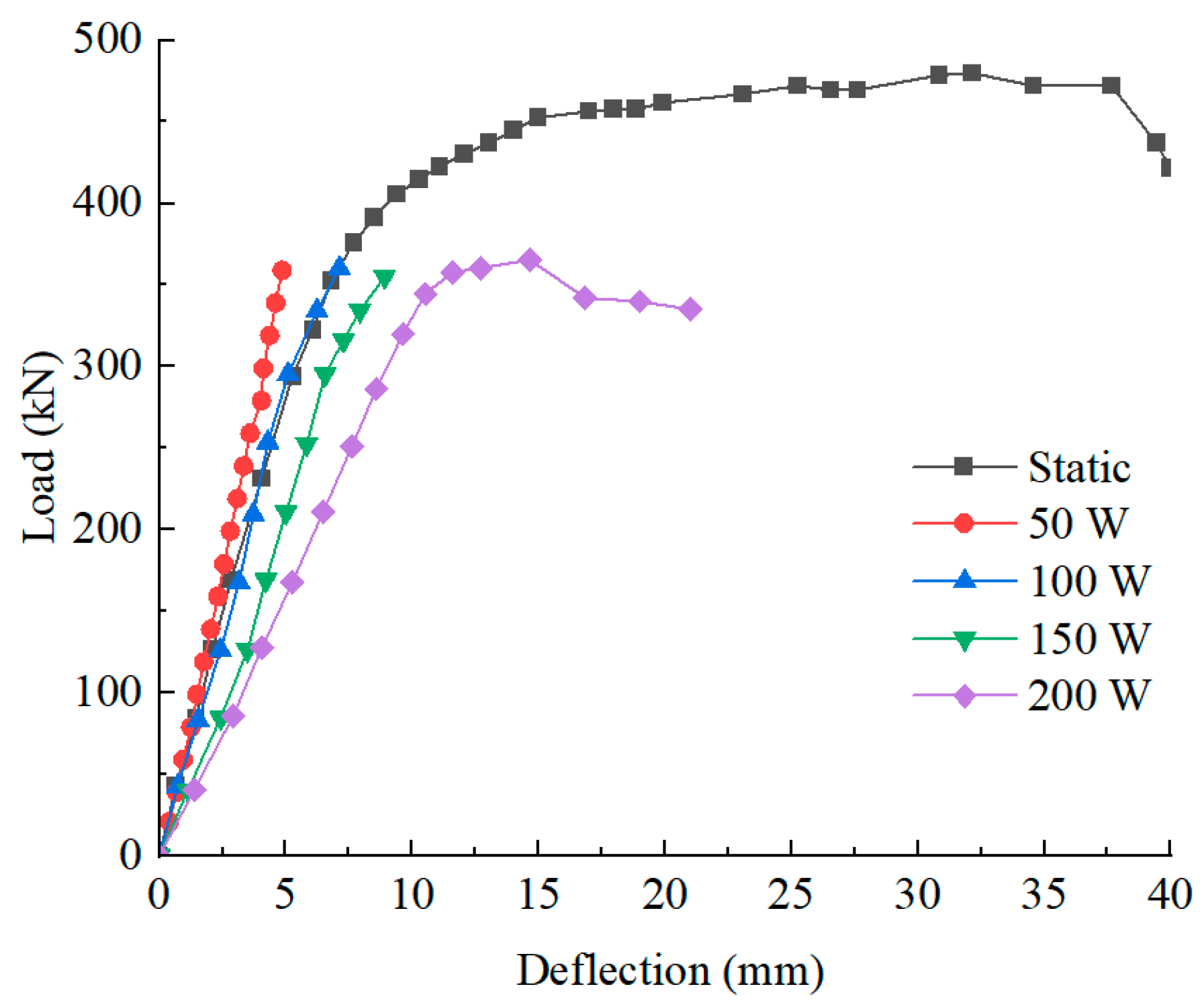
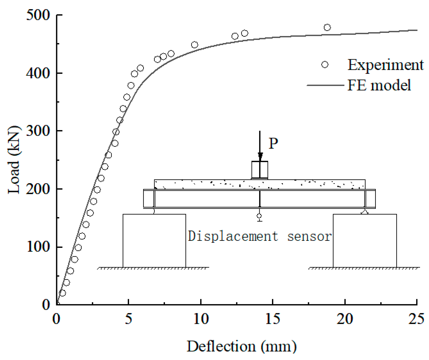
3.2. Load–Deflection Curve

The load–deflection curve is a crucial basis for assessing bending resistance and can reflect the comprehensive performance attributes of composite beams, including stiffness, load-bearing capacity, and ductility, among other key parameters. The following figure illustrates the load–displacement curves for the test beam under static load failure, after a certain number of fatigue cycles during the elastic stage, and after 2 million cycles of cyclic load followed by static load failure [16]. Figure 5 clearly demonstrates the impact of the number of load cycles on the test beam, with both the load-bearing capacity and stiffness during the elastic stage decreasing as the number of cycles increases, as well as ductility diminishing further.

As a result of the low magnitude of cyclic loading, the closure of pores in the concrete material during the initial cycles mitigates the adverse impact of pores on the overall stiffness, thereby densifying the material and, to some extent, enhancing the interaction between the materials. Consequently, this results in an initial increase in the stiffness of the test beams during the early stages of cyclic loading. The ultimate load of the static test beam was about 470 kN, and after being subjected to cyclic loading, the load carrying capacity was about 340 kN, which decreased to 73% of that of the static reference beam, and the reduction in ultimate deflection is even more significant, about 52% of the static reference beam.

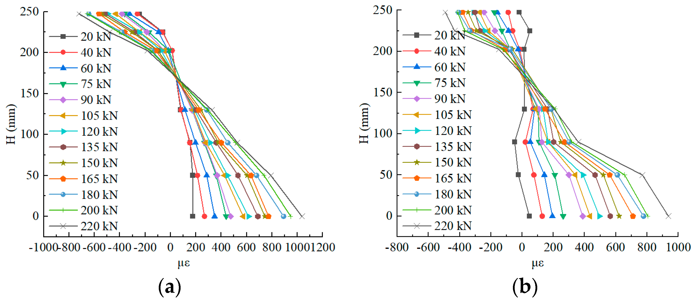
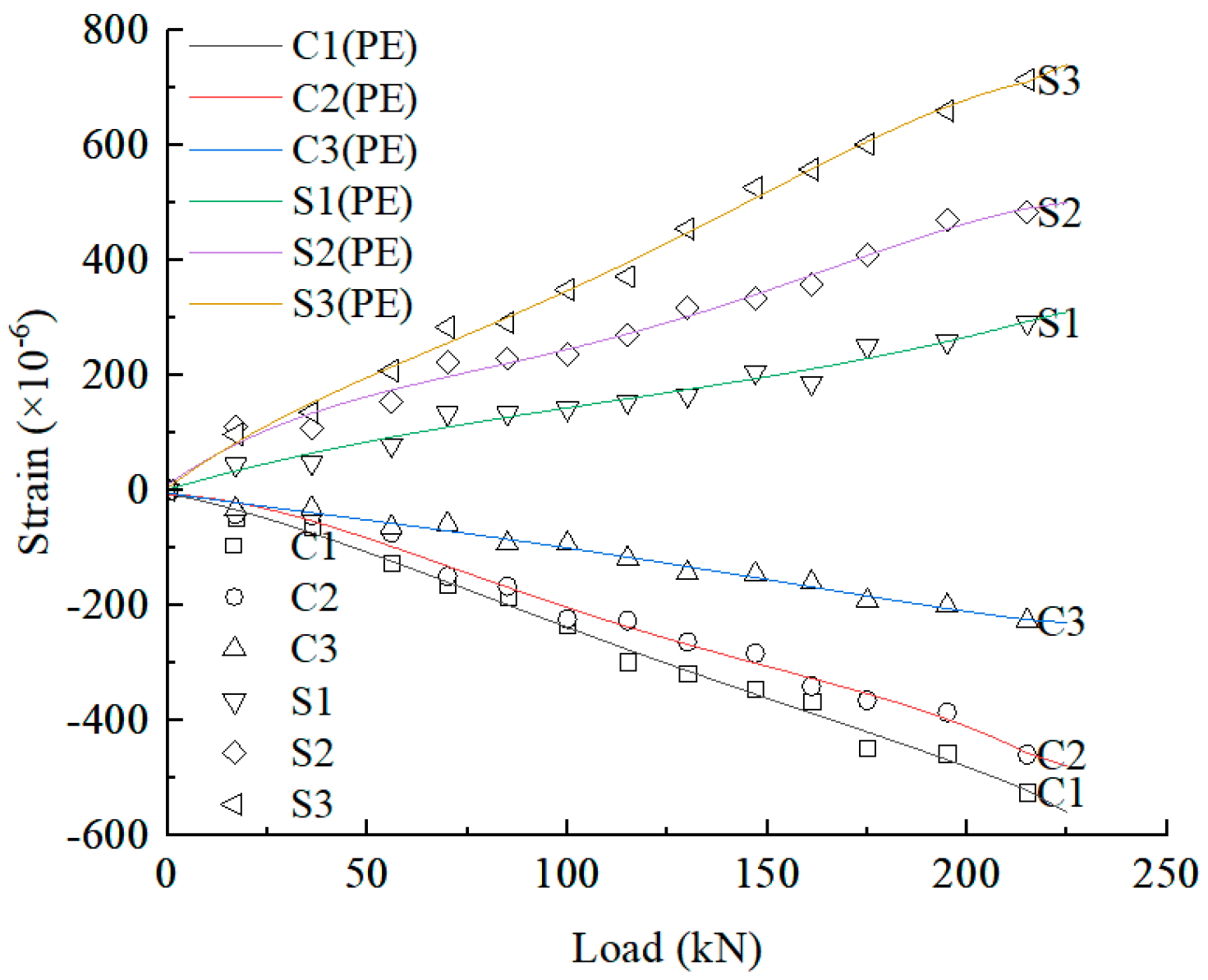
3.3. Load–Section Strain Relationship

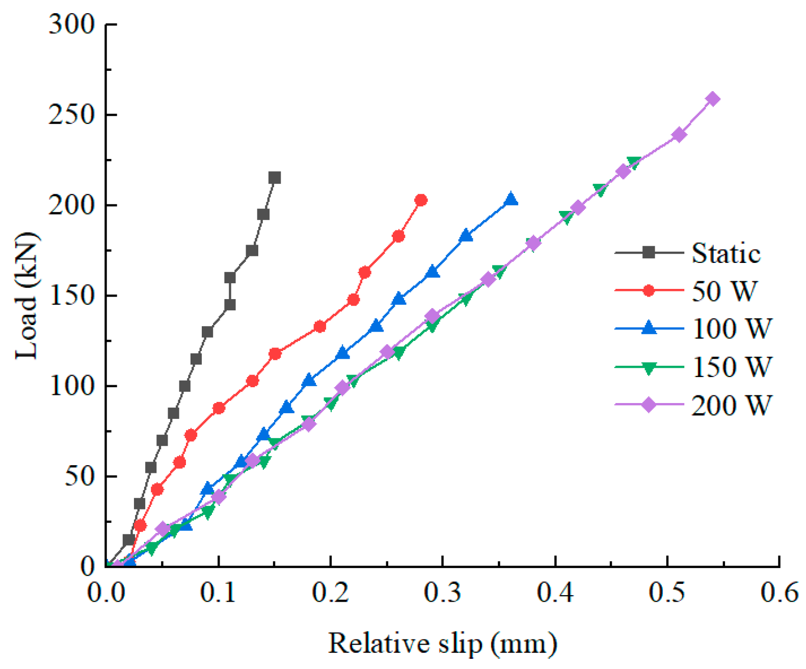
The performance of the composite beams under load can be evaluated from the load–section strain relationship. Figure 6 depicts the load–strain distribution for the mid-span cross-section during the static elastic stage of both static and fatigue test beams. The analysis confirms that both the static and fatigue test beams adhere to the plane section assumption. The static test beam demonstrates superior overall integrity, possessing only one neutral axis. Figure 6b presents the strain distribution of the structure after 150 fatigue load cycles; the diagram shows that, at this point, the cross-section still only has one neutral axis.

3.4. Relative Slip

Stud connectors play a crucial role in steel–concrete composite structures, directly reflecting the synergy between the concrete flange and the steel beam. Figure 7 illustrates the trend of relative slip at the beam end with increasing cyclic loading during the elastic phase tests. From the graph, it can be observed that the variation pattern of relative slip is essentially consistent with the load–deflection curve. The number of cyclic loading cycles is positively correlated with the relative slip of the test beam, indicating that, as the cyclic loading increases, the shear elements gradually fail, and the interface synergy between the concrete slab and the steel beam gradually deteriorates.

The design of stud connectors in the experiment follows the specifications of complete shear connection design. The analysis results indicate that the shear design can meet the mechanical requirements of composite beams under static loading and demonstrate excellent integrity. However, in fatigue tests, with the increase in the number of loading cycles, the shear components are more prone to premature failure compared to the entire beam. Therefore, in future bridge structural designs, especially for composite structures affected by dynamic loads, this aspect should be given special attention.

4. Finite Element Analysis

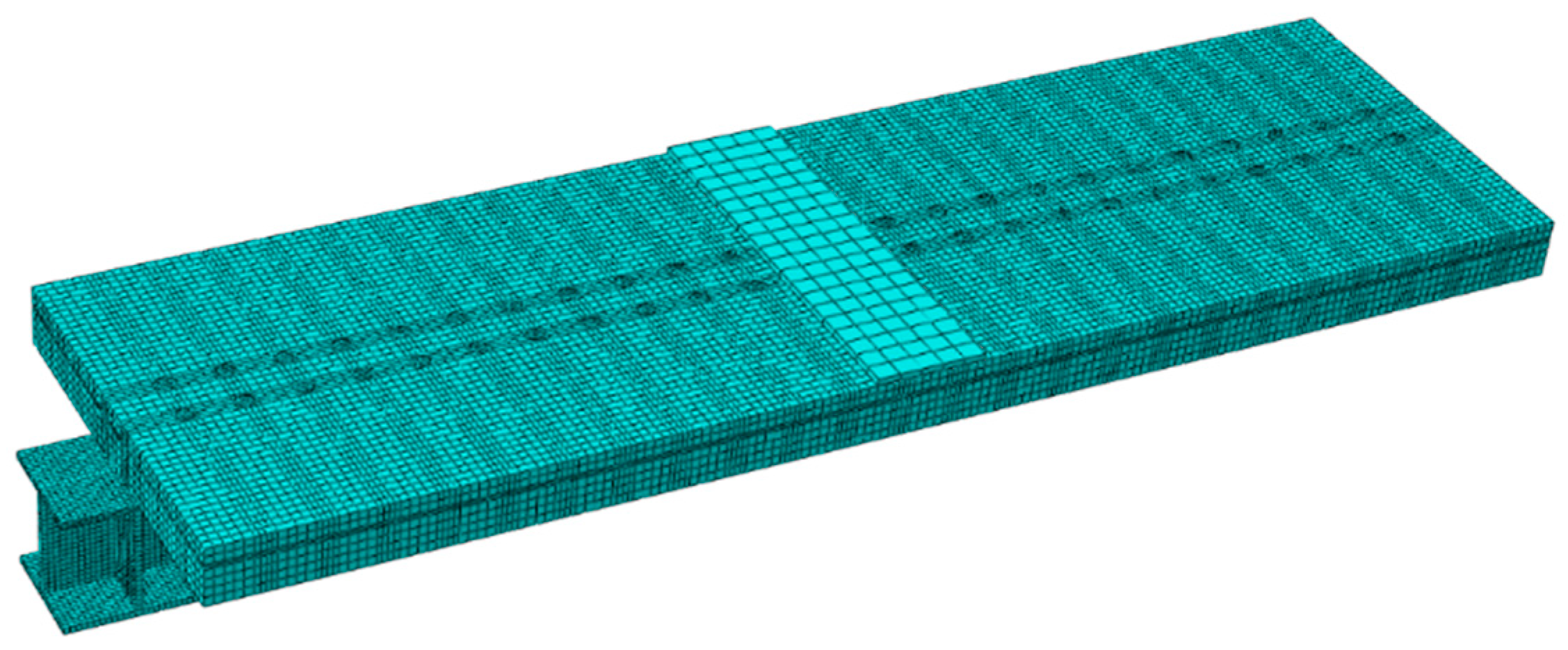
4.1. Establishment of the Finite Element Model

The simulation of a steel–concrete composite test beam model includes a concrete slab, an I-shaped steel beam, stud connectors, rib reinforcements, and rebar configuration. The model is constructed and analyzed using the finite element analysis software ABAQUS (2022). Except for the structural rebar, all components are modeled using solid elements, specifically eight-node linear hexahedral elements (C3D8R), which completely prevent shear locking issues that can occur in integration elements under bending loads. The accuracy of the results is not significantly affected by the shape of the elements, allowing for precise calculations of structural deformations. The rebar is simulated using two-node linear three-dimensional truss elements (T3D2) and is embedded in the concrete slab using a built-in regional approach (see Figure 8).

4.2. Constitutive Relation

The establishment of a finite element model for numerical simulation relies on the selection of the material constitutive model, which determines the accuracy of the model’s computational results. This paper utilizes the built-in parameter settings of Abaqus, adopting the Concrete Damaged Plasticity (CDP) model for the concrete damage model. The constitutive relationship of concrete is defined according to the stress–strain curve calculation formulas for concrete under uniaxial compression and tension, as specified in the GB 50010-2010 [17].

The uniaxial tensile stress–strain curve is calculated using the following equation:

$$\sigma =(1-d_t)E_c\epsilon$$

(3)

$$d_t=\left\{\begin{array}{l}1-{\rho }_t(1.2-0.2x^5)\hspace{1em}x\le 1\\ 1-\frac{{\rho }_t}{{\alpha }_t{(x-1)}^{1.7}+x}\hspace{1em}\hspace{1em} x>1\end{array}\right.$$

(4)

where ${\rho }_t=\frac{f_t^{\ast }}{E_c{\epsilon }_t}$, $x=\frac{\epsilon }{{\epsilon }_t}$, E_c is the modulus of elasticity of concrete, ${\alpha }_t$ is the reference value for uniaxial tensile loading of concrete, $f_t^{*}$ is the uniaxial tensile strength of concrete, ${\epsilon }_t$ is the maximum tensile strain, and $d_t$ is the parameter for the evolution of uniaxial tensile damage in concrete.

The stress–strain curve for uniaxial compression is calculated using the following equation:

$$\sigma =(1-d_c)E_c\epsilon$$

(5)

$$d_c=\left\{\begin{array}{l}1-\frac{{\rho }_{c}n}{n-1+x^n}\hspace{1em}x\le 1\\ 1-\frac{{\rho }_c}{{\alpha }_c{(x-1)}^2+x}\hspace{1em}x>1\end{array}\right.$$

(6)

where ${\rho }_c=\frac{f_c^{\ast }}{E_c{\epsilon }_c}$, $n=\frac{E_c{\epsilon }_c}{E_c{\epsilon }_c-f_c^{\ast }}$, $x=\frac{\epsilon }{{\epsilon }_c}$, ${\alpha }_c$ is the reference value for uniaxial compression of concrete, $f_c^{\ast }$ is the uniaxial compressive strength of concrete, ${\epsilon }_c$ is the corresponding maximum compressive strain of concrete, and $d_c$ is the parameter for the evolution of uniaxial compressive damage in concrete.

The structural steel and stud connectors constitutive relationships utilize a bilinear model. The steel plate used for the experimental beam is Q235 steel. Specific material parameters are listed in the

Table 2. Finite element steel parameters.

Material	fy (MPa)	fu (MPa)	εy	εu
ML-15	440	528	0.002	0.044
Q235	345	450	0.002	0.052

and

Table 3. Concrete plasticity parameters.

Parameter	Expansion Angle (°)	Eccentricity (%)	fb0/fc0	K	Viscosity Parameter
Value	35	0.1	1.16	2/3	0.005

.

Setting the contact nonlinearity between components can better simulate the overall stress changes in the actual experimental beam. Based on the study of the contact model for stud connectors, the contact type between surfaces is set, and the calculated results have a very high agreement with the experimental outcomes. However, by constraining the stud connectors in a tied manner, the accuracy of the calculated results is already sufficient to meet practical needs [18].

4.3. Finite Element Results Analysis

To assess the accuracy of the finite element simulation for structural forces and damage patterns, the simulated damage was compared and analyzed against the experimental damage patterns, as depicted in Figure 9. Upon comparative analysis, the simulation results were found to be highly consistent with the experimental data, with local buckling observed in the steel girder’s span; the concrete slab of the experimental girder also exhibited numerous cracks within the bottom slab’s span.

After performing finite element modeling and analysis, the load–deflection relationship curve at the mid-span position is obtained (see Figure 10). Comparing the simulated numerical relationship with actual data, we see that the results are consistent. The maximum average error for mid-span deflection and the strain gauges on the side of the concrete slab (C1, C2, and C3) and the steel beam (S1, S2, and S3) are all within 5% (see Figure 11). This verifies the reliability of the established finite element model.

4.4. Stress Analysis

Figure 12 illustrates the stress distribution and deformation of steel components under the maximum load amplitude (0.6). Relative to the concrete voids, sliding to the left and downward occurred at the welded position at the bottom of the stud connectors. This reflects the transmission of horizontal and vertical shear forces through the contact pressure on the hole walls from the concrete to the steel beam via the stud connectors, causing considerable compressive stress near the support area at the welded-hole positions. Significant tensile stress also occurs in the lower and left side of the stud connectors, in both the longitudinal and vertical directions near the loaded side. As the position approaches the mid-span, the longitudinal strain gradually decreases due to the change in the direction of force. Additionally, as shear components, the stud connectors overall bear a large amount of shear stress generated by the compression of the entire beam. This indicates that the welded sections in the shear area are in a multiaxial stress state, where longitudinal normal tensile stress, vertical normal tensile stress, and shear stress coexist.

To further understand the overall stress state of the composite beam, three paths parallel to the longitudinal direction were predetermined. Due to the symmetric double-row arrangement of the stud connectors, the curve changes and fatigue damage parameters are quite similar; therefore, only one was selected, namely Path 1 along the center of the longitudinal stud connector welds. Fatigue cracks are also likely to occur near the toe of the stud weld. Path 2 is taken parallel in the same direction along Path 1, and the I-shaped steel beam is constructed from three welded steel plates, with significant bending deformation at the bottom of the beam where the corner welds are also susceptible to damage. Path 3 was chosen accordingly, as illustrated in the Figure 13. Under load amplitudes between 0.35 and 0.6, the longitudinal normal tensile stress amplitude, vertical normal tensile stress amplitude, and shear stress amplitude along these three paths are output.

As can be known from Figure 13, the stress amplitudes fluctuate in a wavelike curve longitudinally, with local peaks near the center of the shear connectors. Among the considered paths, the maximum amplitude of longitudinal normal stress occurs in the bending area of Path 2; the maximum amplitude of vertical normal stress and the maximum shear stress amplitude are located in the shear area of Path 1. This indicates that the effects of vertical normal stress and shear stress become more pronounced as the distance between the weldment and the predefined paths decreases. Furthermore, the highest values of vertical normal stress amplitude and shear stress amplitude are 4.37 times and 1.97 times that of the maximum longitudinal stress amplitude, respectively, suggesting that the amplitudes of vertical normal stress and shear stress are the main factors causing the multiaxial stress state in the weldments.

5. Fatigue Damage Parameter Analysis

5.1. Critical Damage Plane Method

Considering components under multiaxial stress–strain conditions, the critical plane method [19,20] can be utilized to predict the initiation locations of cracks. This method is highly effective in multiaxial fatigue evaluations. It assumes that there exists a critical plane under multiaxial stress states where fatigue damage reaches its maximum, making it more susceptible to fatigue failure. Numerous mature models have been developed for the study of fatigue damage parameters; this paper references the Smith–Watson–Topper (SWT) model to analyze issues related to multiaxial stresses [21]. The parameters are defined as in Equation (5), and the model effectively assesses the impact of mean stress using strain energy [22].

$$D=\frac{\mathsf{\Delta }\epsilon }{2}{\sigma }_{max}$$

(7)

where D indicates the fatigue damage parameters, $\mathsf{\Delta }\epsilon$ represents the amplitude of the normal strain per cycle, and ${\sigma }_{max}$ represents the maximum normal stress during the cycle.

This parameter quantitatively reflects the degree of fatigue failure and damage of the analyzed element under multiaxial stress. On the critical plane, this damage parameter reaches its maximum value. The larger the SWT parameter, the higher the degree of fatigue damage, and the more likely fatigue cracks are to appear.

To confirm the critical plane of a component and identify the most disadvantageous position for calculating the SWT parameter for fatigue life prediction analysis, it is necessary to first calculate the stress–strain field of the component. Using the Abaqus 2022 software, stress and strain data for each element in the global coordinates (x, y, and z) are output. The coordinate system (x’, y’, and z’) used for calculations is derived from the matrix shown in Figure 14. This determines the critical plane and the most disadvantageous load position. The calculation formula for each element on the plane is as follows:

$$\sigma ={\sigma }_{xx}{n}_x^2+{\sigma }_{yy}{n}_y^2+{\sigma }_{zz}{n}_z^2+2{\tau }_{xy}{n}_x{n}_y+2{\tau }_{yz}{n}_y{n}_z+2{\tau }_{xz}{n}_x{n}_z$$

(8)

$$\epsilon ={\epsilon }_{xx}{n}_x^2+{\epsilon }_{yy}{n}_y^2+{\epsilon }_{zz}{n}_z^2+2{\gamma }_{xy}{n}_x{n}_y+2{\gamma }_{yz}{n}_y{n}_z+2{\gamma }_{xz}{n}_x{n}_z$$

(9)

In the formula, the stress and strain are the transformed normal stress and strain, where n_x, n_y, and n_z are the direction cosines of the plane normal relative to the global coordinates. These are calculated using Equations (8)–(10):

$$n_x=cos\theta sin\phi$$

(10)

$$n_y=sin\theta sin\phi$$

(11)

$$n_z=cos\phi$$

(12)

where θ is the angle between the z-axis and the projection of the plane normal on the xy-plane, and ϕ is the angle between the plane normal and the z-axis. After calculating the values of θ and ϕ, the verification plane with the maximum SWT parameter calculated using Equation (5) is considered the critical plane.

The specific calculation values consider that the SWT damage parameter is a function of θ and φ. The calculation is made by taking values for the angle from 0° to 180° at intervals of 10°, analyzing a 180 × 180 plane. For example, Figure 15 shows the SWT parameters of an element on Path 1, approximately 80 mm from the support edge of the specimen, at various θ and φ angles. When θ and φ are at 40° and 90°, respectively, the maximum fatigue damage parameter is 1.22 × 10⁵. Thus, the plane at 40° θ and 90° φ is the critical plane for this element, and 1.22 × 10⁵ is the fatigue damage parameter on this critical plane, which is also the SWT parameter for the element. Subsequent analyses also determined that fatigue cracks began to propagate from this location.

5.2. Parameter Analysis

Figure 16 shows the longitudinal distribution of SWT parameters for components along paths 1, 2, and 3 under a load amplitude of 0.25, and the maximum SWT parameters are shown for each path. Numerical and graphical comparisons indicate that, compared to other surfaces and interface connections, the most disadvantageous load positions are mostly concentrated at the locations of stud connectors, where the fatigue damage parameters are significantly greater. This confirms that shear connectors are key to the study of the fatigue performance of the experimental beam. The most likely locations for fatigue cracks to occur and for fatigue failure to happen are at the stud positions at the far-left end of the beam, where the shear is greatest. These analytical positions are in very close agreement with the results observed in the experiment where significant deformation occurred, indicating that the stud welding areas are the primary sources of fatigue damage in composite beam components.

In the experiments, apart from fatigue cracks leading to structural failure at the toe of the welds, shear failure of the studs could also occur. Therefore, an SWT parameter analysis was conducted on the studs at the most disadvantageous load positions along Path 1 in terms of circumferential direction and vertical height to determine the overall most disadvantageous load positions of the studs, as shown in Figure 17.

In practical engineering, defects in composite structures can arise due to issues related to the preparation, transportation, or inherent quality of concrete, thereby affecting the mechanical performance of the structure [23,24]. To further verify the reliability of the analysis process described above, this paper calculates the distribution of SWT parameters for four groups of specimens with certain initial defects [25]. The introduction of initial defects is primarily handled in two ways: actual measurement and the use of buckling mode-related initial defects. This paper employs the former method and changes the corresponding numerical values of the components to achieve the relevant simulations [26]. The specimen parameters are listed in

Table 4. Initial defect parameter.

Porosity (%)	Specimen Number	Aperture (mm)	fckn/fck	Ecn/Ec
1	K1-0.3	0.3–0.6	0.957	0.962
	K1-3	3–5	0.868	0.959
	K1-5	6–8	0.834	0.945
	K1-8	8–10	0.815	0.924
4	K4-0.3	0.3–0.6	0.892	0.942
	K4-3	3–5	0.781	0.920
	K4-5	6–8	0.770	0.901
	K4-8	8–10	0.764	0.888
7	K7-0.3	0.3–0.6	0.7955	0.878
	K7-3	3–5	0.675	0.839
	K7-5	6–8	0.651	0.801
	K7-8	8–10	0.639	0.776
10	K10-0.3	0.3–0.6	0.698	0.809
	K10-3	3–5	0.587	0.776
	K10-5	6–8	0.571	0.761
	K10-8	8–10	0.564	0.748

.

During the calculation process, the three chosen analytical paths indicate that the shear connector key is most likely to develop fatigue cracks. Moreover, the maximum fatigue damage parameter is found in the tensile zone of the shear connector key at the beam’s end. Consistent with the most adverse experimental findings on shear connector keys in simply supported beam specimens by Wang [15] and Xing [16], this confirms that the established finite element model and the critical plane method based on SWT parameters can reliably evaluate the initiation locations of fatigue cracks in steel–concrete composite beams. The results, as shown in Figure 18, indicate, through a graphical trend analysis, that an increase in porosity and pore size not only leads to a decrease in the overall load-bearing capacity of the experimental beam but also continuously increases the fatigue damage parameters, making the beam more susceptible to fatigue cracking and failure. The rate of change in the slope indicates that, under the same pore size, an increase in porosity has a greater impact on the damage parameters of the experimental beam compared to an increase in pore size under the same porosity level.

Considering the impact of porosity defects on the fatigue performance of the experimental beam, as illustrated in Figure 18b, the growth rate of SWT parameters is slower than the rate of reduction in concrete strength. This is because, as a composite beam, the components transfer forces among each other and compensate for the reduction in overall performance caused by the decreased concrete strength. Moreover, compared to pore size, changes in porosity have a more significant impact on the overall damage parameters. For example, at a porosity of 1% and a pore size between 0.3 and 0.6 mm, the damage parameter, D, increased by 1.7%. When the porosity increased to 10%, D increased by 23.5%. When the porosity was 1% and the pore size increased to 8–10 mm, D increased by 11.7%. When both the pore size and porosity are too large, there is a reduction in the SWT parameters, which is due to the insufficient restraint provided to the bolts by the overly weakened concrete, leading primarily to concrete spalling.

6. Conclusions

This study conducted experiments and numerical simulations by using the multiaxial fatigue critical plane calculation method to explore the mechanical performance variations and failure mechanisms of steel–concrete composite beams.

(1)

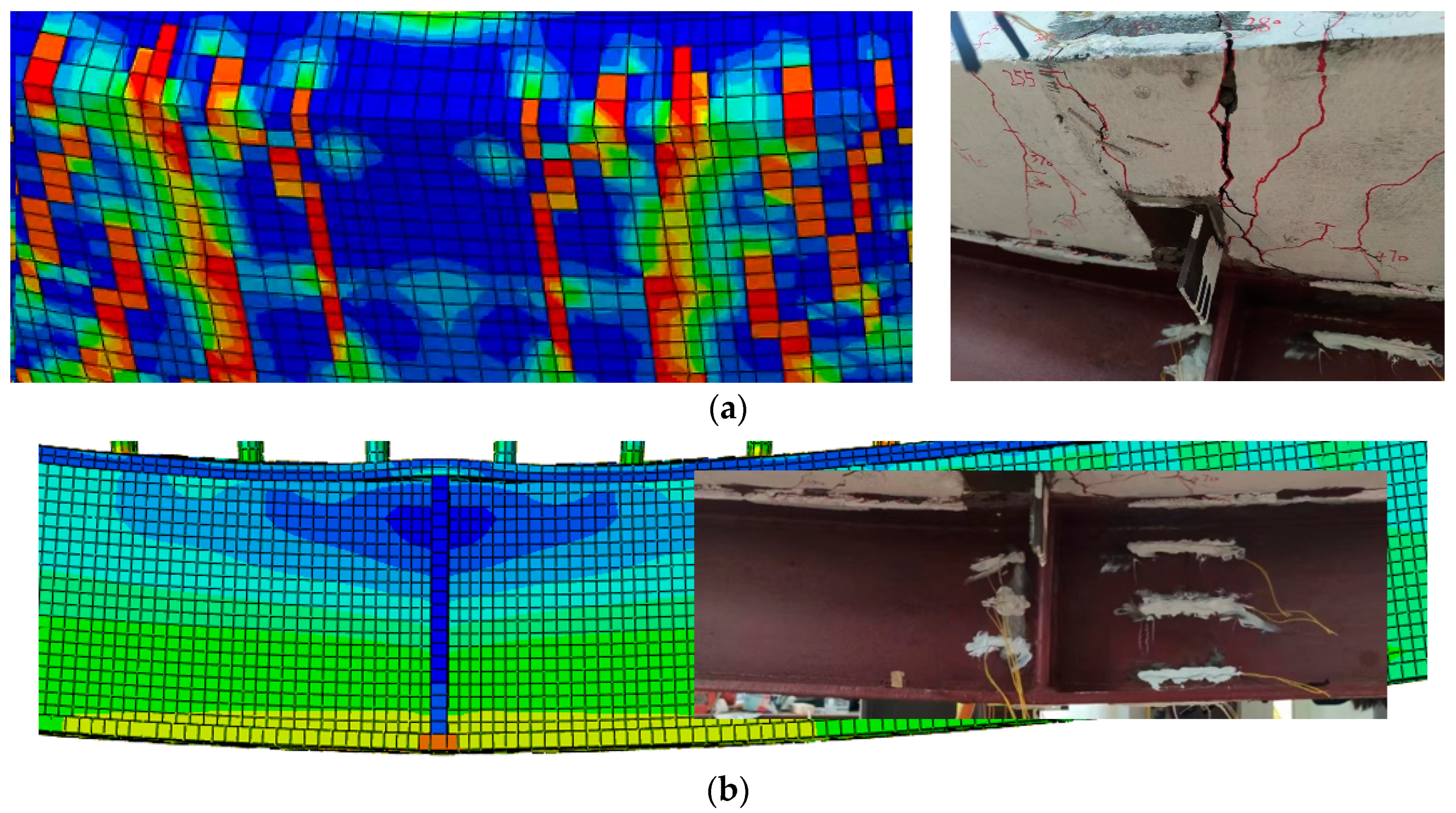
The fatigue failure process of the steel–concrete composite beams begins with plastic deformation occurring in the welded joints, followed by the concrete slab undergoing hundreds of thousands of fatigue load cycles until the concrete strength reaches its limit and starts to spall until failure.

(2)

By integrating experimental data and a nonlinear material constitutive defined by formulas, key positions within the finite element model can be finely modeled, effectively simulating the load–slip curve and stress–strain values of the steel–concrete composite beams. Additionally, the use of finite element simulation provides a more intuitive understanding of those disadvantageous positions that are typically difficult to observe experimentally.

(3)

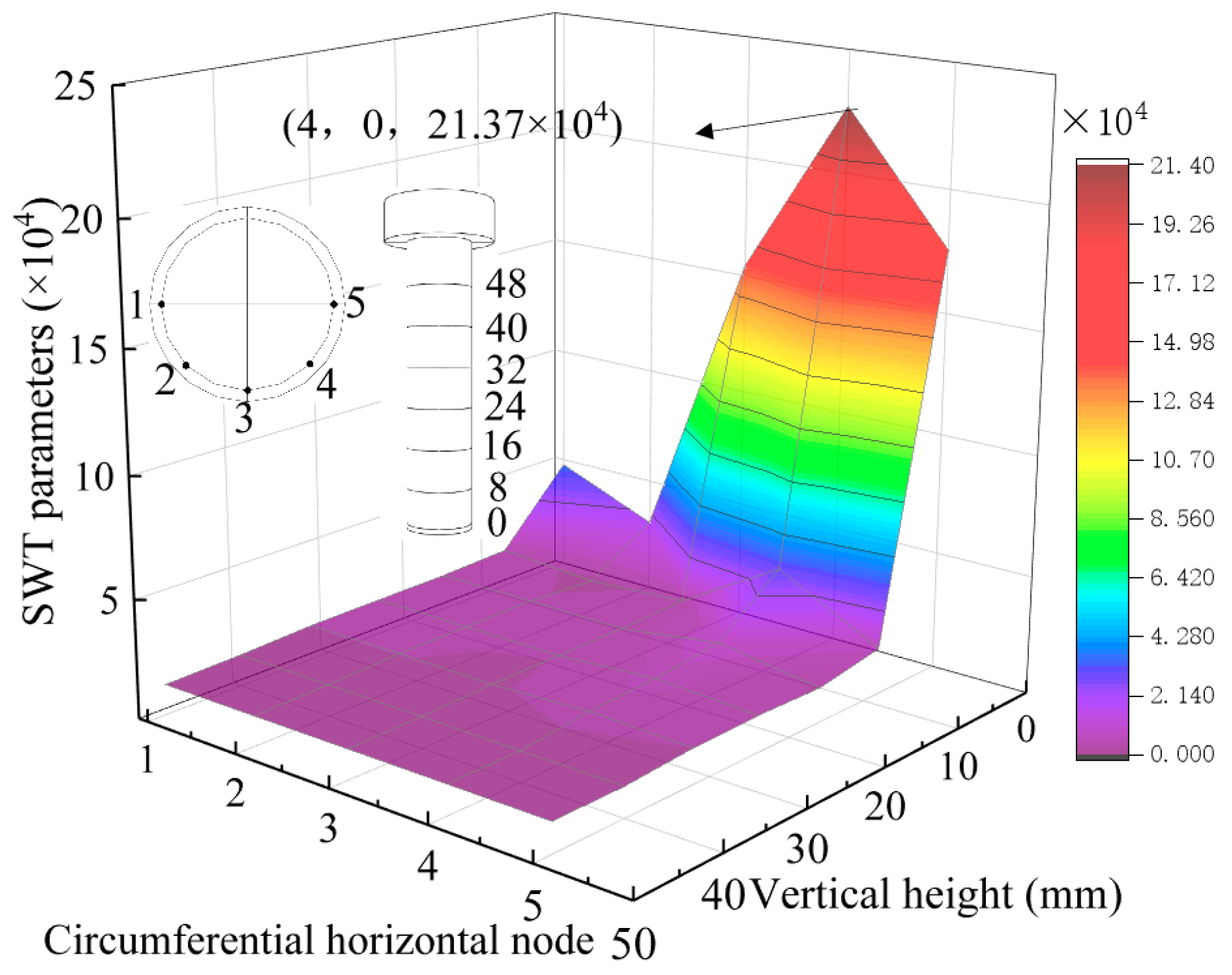
The finite element analysis shows that the shear transfer between components and the welded parts in the shear zone are in a multiaxial stress state, where longitudinal normal stress, vertical normal stress, and shear stress coexist. Observations and calculations of fatigue damage parameters at the most disadvantageous load positions are essentially consistent; thus, using the critical plane method based on SWT parameters to evaluate and predict the fatigue locations of components is reliable.

(4)

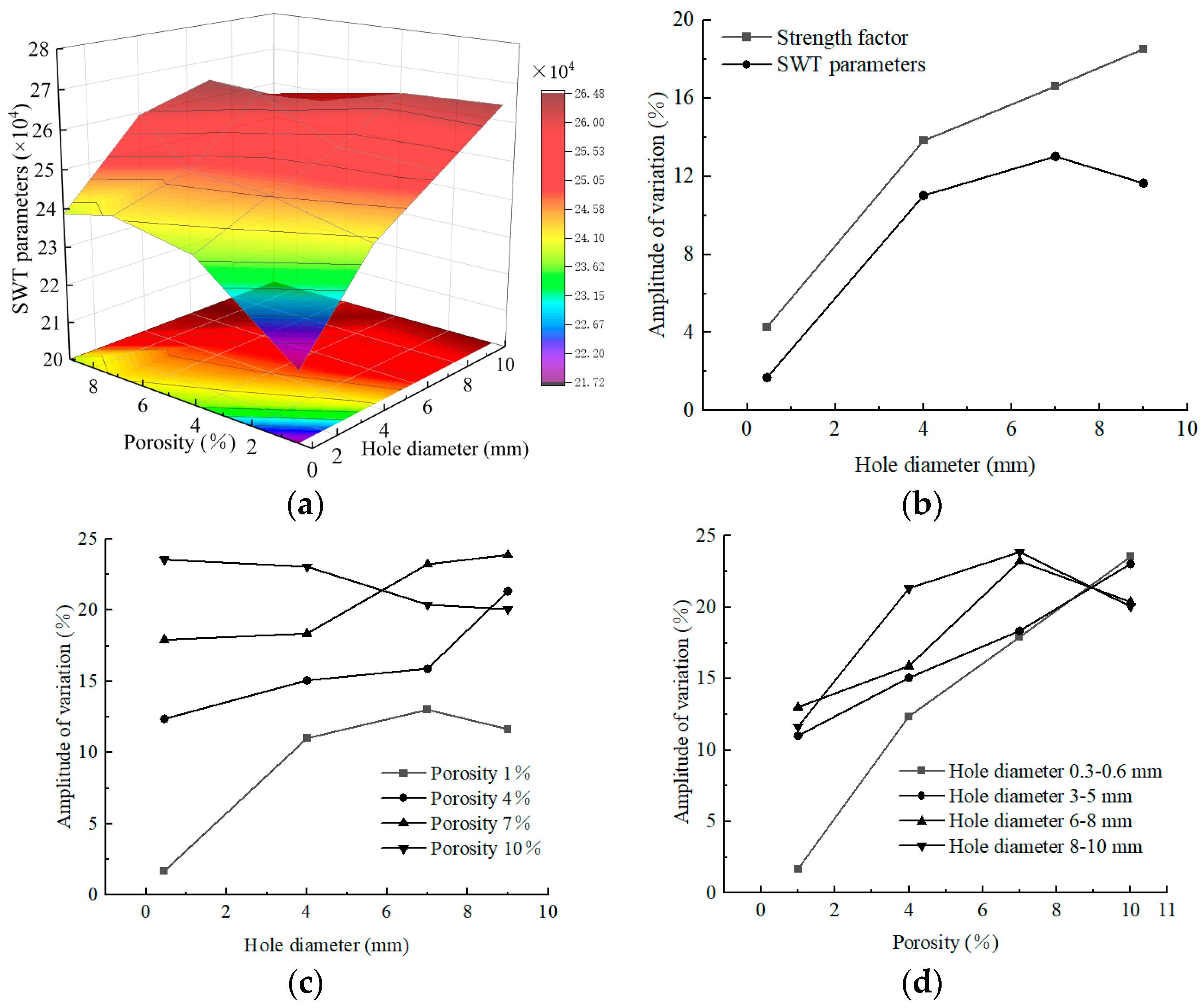
Fatigue damage parameters indicate that the most disadvantageous loading plane of the experimental beam is in the shear zone, and the stud weld toes, which experience the highest tensile stress, are more susceptible to fatigue cracking compared to the contact surfaces. Setting initial porosity defects, the performance impact caused by them is offset by the various components of the composite beam, with the growth in damage parameters being less than the strength reduction rate. The variation in component porosity has a more significant impact on the overall damage parameters than the pore size, which requires more attention in engineering applications.

References

1. Wang, D.; Tan, B.; Zhao, P. Experimental and numerical study of temperature gradient effect on behavior of steel-concrete composite bridge deck. J. Build. Struct. 2021, 42, 74–82. [Google Scholar]
2. Zou, Y.; Jiang, J.; Yang, J.; Zhang, Z.; Guo, J. Enhancing the toughness of bonding interface in steel-UHPC composite structure through fiber bridging. Cem. Concr. Compos. 2023, 137, 104947. [Google Scholar] [CrossRef]
3. Cao, X.; Cheng, C.; Wang, M.; Zhong, W.; Kong, Z.; Chen, Z. Experimental study on the flexural behavior of flat steel-concrete composite beam. Can. J. Civ. Eng. 2020, 48, 1155–1168. [Google Scholar] [CrossRef]
4. Zeng, Y.; Yu, T.; Xiao, Y.; Li, W. Investigation of the Mechanical Features of Steel–Concrete Composite Girder Rigid Frame Bridges with V-Shaped Piers during Construction Stages. Appl. Sci. 2024, 14, 3343. [Google Scholar] [CrossRef]
5. Silva, M.L.d.; Prado, L.P.; Félix, E.F.; Sousa, A.M.D.d.; Aquino, D.P. The Influence of Materials on the Mechanical Properties of Ultra-High-Performance Concrete (UHPC), A Literature Review. Materials 2024, 17, 1801. [Google Scholar] [CrossRef] [PubMed]
6. Wang, D.; Zheng, Z.; Xu, Z.; Yan, W.; Zhang, B. Study on the effect of length of bolted connectors on shear bearing capacity in steel-mixed composite structures. Highw. Mot. Transp. 2022, 4, 97–100+105. [Google Scholar]
7. Wu, Y.; Wang, X.; Fan, Y.; Shi, J.; Luo, C.; Wang, X. A Study on the Ultimate Span of a Concrete-Filled Steel Tube Arch Bridge. Buildings 2024, 14, 896. [Google Scholar] [CrossRef]
8. Burhan, I.; Kim, H.S. S-N Curve Models for Composite Materials Characterisation, An Evaluative Review. J. Compos. Sci. 2018, 2, 38. [Google Scholar] [CrossRef]
9. Motte, R.; De Waele, W. An Overview of Estimations for the High-Cycle Fatigue Strength of Conventionally Manufactured Steels Based on Other Mechanical Properties. Metals 2024, 14, 85. [Google Scholar] [CrossRef]
10. Wang, D.; Tan, B.; Xiang, S.; Wang, X. Fatigue crack propagation and life analysis of stud connectors in steel-concrete composite structures. Sustainability 2022, 14, 7253. [Google Scholar] [CrossRef]
11. Xiang, D.; Gu, M.; Zou, X.; Liu, Y. Fatigue behavior and failure mechanism of steel-concrete composite deck slabs with perforated ribs. Eng. Struct. 2022, 250, 113410. [Google Scholar] [CrossRef]
12. Łagoda, T.; Vantadori, S.; Głowacka, K.; Kurek, M.; Kluger, K. Using the Smith-Watson-Topper Parameter and Its Modifications to Calculate the Fatigue Life of Metals, The State-of-the-Art. Materials 2022, 15, 3481. [Google Scholar] [CrossRef] [PubMed]
13. Li, X.; Yang, H.; Yang, J. Fretting Fatigue Life Prediction for Aluminum Alloy Based on Particle-Swarm-Optimized Back Propagation Neural Network. Metals 2024, 14, 381. [Google Scholar] [CrossRef]
14. Branco, R.; Costa, J.D.; Prates, P.A.; Berto, F.; Pereira, C.; Mateus, A. Load sequence effects and cyclic deformation behaviour of 7075-T651 aluminium alloy. Int. J. Fatigue 2022, 155, 106593. [Google Scholar] [CrossRef]
15. Wang, B.; Huang, Q.; Liu, X. Comparison of static and fatigue behaviors between stud and perfobond shear connectors. KSCE J. Civ. Eng. 2019, 23, 217–227. [Google Scholar] [CrossRef]
16. Xing, Y.; Han, Q.; Xu, J.; Guo, Q.; Wang, Y. Experimental and numerical study on static behavior of elastic concrete-steel composite beams. J. Constr. Steel Res. 2016, 123, 79–92. [Google Scholar] [CrossRef]
17. GB 50010-2010; Code of Design Concrete Structures. China Construction Industry Press: Beijing, China, 2011; pp. 209–211.
18. Wang, B.; Liu, X.; Zhu, P. Residual bearing capacity of steel-concrete composite beams under fatigue loading. Struct. Eng. Mech. 2021, 77, 559–569. [Google Scholar]
19. Arora, P.; Gupta, S.K.; Samal, M.K.; Chattopadhyay, J. Validating generality of recently developed critical plane model for fatigue life assessments using multiaxial test database on seventeen different materials. Fatigue Fract. Eng. Mater. Struct. 2020, 43, 1327–1352. [Google Scholar] [CrossRef]
20. Wu, Z.; Hu, X.; Song, Y. Multiaxial fatigue life prediction for titanium alloy TC4 under proportional and nonproportional loading. Int. J. Fatigue 2014, 59, 170–175. [Google Scholar] [CrossRef]
21. Smith, K.N.; Watson, P.; Topper, T.H. A stress–strain functions for the fatigue of metals. J. Mater. 1970, 5, 767–778. [Google Scholar]
22. Kujawski, D. A deviatoric version of the SWT parameter. Int. J. Fatigue 2014, 67, 95–102. [Google Scholar] [CrossRef]
23. Vicente, M.A.; González, D.C.; Mínguez, J.; Tarifa, M.; Ruiz, G.; Hindi, R. Influence of the pore morphology of high strength concrete on its fatigue life. Int. J. Fatigue 2018, 112, 106–116. [Google Scholar] [CrossRef]
24. Chandrappa, A.K.; Biligiri, K.P. Effect of pore structure on fatigue of pervious concrete. Road Mater. Pavement Des. 2019, 20, 1525–1547. [Google Scholar] [CrossRef]
25. Cui, W.; Liu, M.; Song, H.; Guan, W.; Yan, H. Influence of initial defects on deformation and failure of concrete under uniaxial compression. Eng. Fract. Mech. 2020, 234, 107106. [Google Scholar] [CrossRef]
26. Lv, C.; Wang, K.; Zhao, X.; Wang, F. Damage-Accumulation-Induced Crack Propagation and Fatigue Life Analysis of a Porous LY12 Aluminum Alloy Plate. Materials 2024, 17, 192. [Google Scholar] [CrossRef]
Figure 1. Sectional dimensions of composite beams: (a) longitudinal section and (b) cross-section.
Buildings 14 01601 g001
Figure 2. Schematic diagram of the calculation of the second type of cross-section.
Buildings 14 01601 g002
Figure 3. Test beam loading: (a) loading diagram, (b) measurement points layout, and (c) loading site diagram.
Buildings 14 01601 g003
Figure 4. Experimental destruction phenomena: (a) transverse cracks, (b) diagonal cracks, (c) longitudinal through cracks, and (d) concrete spalling.
Buildings 14 01601 g004
Figure 5. Mid-span load deflection curve.
Buildings 14 01601 g005
Figure 6. Load–section strain relationship in midspan: (a) static beam and (b) fatigue beam.
Buildings 14 01601 g006
Figure 7. Relative slip curve.
Buildings 14 01601 g007
Figure 8. Calculation model of test beam.
Buildings 14 01601 g008
Figure 9. Comparison of simulated and tested damage patterns: (a) concrete slab damage pattern and (b) steel beam damage pattern.
Buildings 14 01601 g009
Figure 10. Load–mid-span deflection.
Buildings 14 01601 g010
Figure 11. Mid-span load–strain.
Buildings 14 01601 g011
Figure 12. Stress distribution in welded parts: (a) longitudinal normal stress, (b) vertical normal stress, (c) shear stress.
Buildings 14 01601 g012
Figure 13. Stress amplitude of welded parts: (a) calculation paths, (b) longitudinal normal stress, (c) vertical normal stress, and (d) shear stress.
Buildings 14 01601 g013
Figure 14. Arbitrary plane position conversion diagram.
Buildings 14 01601 g014
Figure 15. SWT parameters for θ and φ.
Buildings 14 01601 g015
Figure 16. Distribution of SWT parameters.
Buildings 14 01601 g016
Figure 17. SWT parameter distribution at position of stud.
Buildings 14 01601 g017
Figure 18. SWT parameter relationship of each model: (a) SWT parameters; (b) comparison of strength and SWT parameter drop at 1% porosity; (c) variation curve of SWT parameter increase with the same porosity; and (d) variation curve of SWT parameter increase for the same hole diameter.
Buildings 14 01601 g018