Abstract
Actual load identification is a most important task solved in the course of (1) engineering inspections of steel structures, (2) the design of systems rising or restoring the bearing capacity of damaged structural frames, and (3) structural health monitoring. Actual load values are used to determine the stress–strain state (SSS) of a structure and accomplish various engineering objectives. Load identification can involve some uncertainty and require soft computing techniques. Towards this end, the article presents an integrated method combining basic provisions of structural mechanics, machine learning, and artificial neural networks. This method involves decomposing structures into primitives, using machine learning data to make projections, and assembling structures to make final projections for steel frame structures subjected to elastic strain. Final projections serve to identify parameters of point forces and loads distributed along the length of rods. The process of identification means checking the difference between (1) weight coefficient matrices applied to unit loads and (2) actual loads standardized using maximum load values. Cases of neural network training and parameters identification are provided for simple beams. The aim of this research is to enhance the reliability and durability of steel structures by predicting consequences of unfavorable load, including emergency impacts. The novelty of this study lies in the co-use of artificial intelligence elements and structural mechanics methods to predict load parameters using actual displacement curves of structures. This novel approach will enable engineering inspection teams to predict unfavorable load peaks, prevent emergency situations, and identify actual causes of emergencies triggered by excessive loading.
1. Introduction
Load parameters are identified during engineering inspections of bearing elements, and the reconstruction and renovation of buildings and structures. In some cases, using structural monitoring systems and software packages is problematic, expensive, or technically challenging. Therefore, some researchers recommend artificial intelligence (AI) models, including machine learning-powered techniques. Let us focus on these works.
In some restructuring projects, fiber concrete is used to repair damage in standard concrete. Several experiments were conducted, and numerical modeling was performed to study the bond between these types of concrete for various design parameters. A machine learning regression model was developed to predict the bond strength and effectiveness of this method []. Concrete and reinforced concrete structures, strengthened with carbon fiber-reinforced plastic (CFRP), have complex strain and failure patterns that need simplified predictive models rather than complicated finite-element analyses and experiments [,]. In [], such models are (1) a neural network, (2) a heuristic search optimization algorithm simulating the behavior pattern of a bee colony, and (3) Gaussian process regression. Fiber-reinforced mortar can be used to repair and restore building structures. It can be injected into openings or used to fill concrete masonry joints. Uncertainty about bond strength values and mechanical characteristics of materials make this type of masonry too complex to analyze. To find the bond strength in a similar problem, authors of [] used several widespread machine learning models, of which Gaussian process regression was the most effective. Publication [] focuses on using carbon fiber lamellas to effectively strengthen structures. Two ensemble learning models (a random forest and a gradient decision tree) predict the strength of the bond between carbon fiber-reinforced polymer and concrete. Machine learning is effectively used to identify cracks in concrete and reinforced concrete structures. Photographs of cracks made in the course of experiments can serve as a training set to ensure unambiguous identification. In the work [], support vectors serve as the basis for classification used to distinguish bending, shear and compression-triggered cracks. Authors of work [] offer a method to identify cracks, inclusions, pits, and scratches. Modified deep learning approaches and a transformed ordinary convolutional network can identify combinations of defects. The authors of the work [] continued studying different types of damage in flat single-story frames. Nodal connections in frame systems and their damage under seismic load are considered there. The reaction of a structure with an experimentally damaged beam–column joint serves as a reference.
The condition of bolted connections in steel frames is monitored in the work []. A hybrid method of interacting models is used there. A machine learning model, composed of support vectors, is trained to identify loose and tight bolted connections. Data on the vibration of bolted connections for a certain period of time are collected there. These data are further used to update stiffness values in a finite-element model and make a conclusion about the degree of hazard from the stress state of a steel frame structure as a whole.
Work [] focuses on co-using (1) a calibrated finite-element model, adjustable to environmental conditions, and (2) a machine learning model to monitor and evaluate bridge structures.
Machine learning is used in conjunction with a digital twin technology [] to monitor individual structures at the stage of operation. This approach can be employed to simulate emergency impacts, including those affecting pre-stressed steel structures. The frequency of vibrations in structural elements and its change in time determine the extent of damage to steel structures identified in the course of structural health monitoring, which is needed to check the technical condition of a structure []. Images of such graphs can be recognized by means of (1) support vectors and (2) clustering the most relevant damage identifiers using the algorithm of the K-nearest neighbors. Work [] elaborates on analyzing damage in steel structures. Cracks are identified by applying a stress intensity factor. Model training is based on the finite-element method, while the prediction model itself is based on the Gaussian process. An improved damage identification method is proposed in []. It is noteworthy that the accuracy of damage type prediction, based on widespread machine learning methods, relies on the quality and quantity of data. The task of evaluating the technical condition of structures after emergency impacts is highly relevant. A support vectors method, a naive Bayesian classifier of the Gaussian-type, and neural networks are used in [] for this purpose. Structural health monitoring is also conducted there. It ties emergency damage to the system stiffness and strain values. Strain data were obtained during supplementary load testing.
An algorithm designed for monitoring and evaluating the technical condition of high-rise buildings is proposed in the work []. After the interrogation of sensors, recorded signals undergo the Fourier transform. Further, wavelet transformation is applied to remove noise from signals directed into the neural network as input data. Particular features are extracted from signals and classified using the neural network. This classification includes several types of damage: minor damage, moderate damage, and collapse. Data collected over the last ten years were analyzed to improve the efficiency of damage monitoring in load-bearing structures and to make a hierarchical classification of damage types []. As a result, artificial and convolutional neural networks, as well as support vectors, proved to be highly efficient and accurate. No detailed analysis of each work is needed to make the conclusion that loads and components of the stress–strain state are identified with the help of artificial intelligence in works on seismic risk analysis [,,,] and in works on the evaluation of building operation modes and information modeling [,,,].
The difference between predicted and observed values should be minimized in the process of training models to predict complex processes. Here, heuristic optimization methods are used, for example, in the works [,]. However, their use is limited by the need to make numerical or analytical calculations to obtain complex process data. In this case, some simplifications can be made, for example, by reducing the LOD (levels of detail) in models [,].
Displacement identification is a truly relevant task today. Methods of predicting the displacement of soil, slopes and structures are investigated in [,,,]; the displacement of bearing structures is addressed in [,,].
The task of displacement identification is part of structural health monitoring, which is the focus of several studies. Steel frame structures are addressed in the article [], which compares different advanced machine learning models designed to evaluate the seismic response of multi-story buildings. This approach is extended in [] by the soil-structure interaction. A prediction is also made for structural health monitoring purposes in cases of seismic actions on reinforced concrete structures [].
In addition, it is extremely important to consider both natural and human-induced effects. For example, enhancing the reliability of steel structures is crucial in case of explosions. Such impacts can be particularly dangerous for columns [,] and elements of artificial intelligence are employed to derive analytical dependencies to evaluate their load-bearing capacity.
This literature review demonstrates that machine learning is widely used to solve various tasks in the construction industry, and the main areas of focus are as follows: (1) structural health monitoring, digital twins for civil, industrial, and bridge structures; (2) evaluating the seismic stability of buildings and built-up areas, minimizing risks of socio-economic losses; (3) predicting strain and failure processes, including interaction with soil; (4) identifying optimal solutions based on a combination of heuristic algorithms with AI technologies, including ensemble learning methods.
This article proposes a new alternative approach to displacement identification. This approach represents a complex structure as a set of substructures for which training is performed.
The aim of this research is to enhance the reliability and durability of steel frame structures by predicting consequences of unfavorable loading, including emergency impacts. The following tasks should be solved to achieve this goal: (1) formulating the general concept for predicting load parameters based on the decomposition of a complex system into simple rods; (2) adapting and implementing the proposed concept using standard profile steel elements with uniform cross-sections; (3) developing a supervised learning procedure for these simple rods with the nodal load transfer pattern taken into account, and performing the training in respect of widespread types of unit loads; (4) performing a practical verification of the ability to spot the load and to determine its value.
2. Problem Statement and Methods
2.1. The General Concept of the Computation Process
The strain state of a 3D finite-element model of a structure can be described by a set of displacement vectors in each of its nodes:
- are linear nodal displacements i in the global coordinate system;
- are angular displacements of this node;
- are displacements caused by the dead weight of a structure;
- are displacements triggered by the payload.
Displacement components are nonzero to avoid mathematical uncertainty when weight coefficients describing deflection curves are calculated. That is why support nodes and nodes, having single support links, are disregarded. When 2D systems and systems with displacement evaluation by one degree of freedom are considered, sets are made using arrays of appropriate size. For example, the system has three nodes, and load will only be identified by vertical displacements. Let the y-axis be directed vertically, then, if conditions of Expression (1) are satisfied, the expression can be written as follows: .
A certain model of data associated with a node of a finite-element model is assumed to be a network neuron. In the event of a mechanical action, a displacement vector, associated with a finite-element node, will be understood as an input signal received by a neuron. Hence, each neuron has indirect connections with other neurons that are similar to connections between all nodes in case of deflections of structural elements. Similar to displacements in a neuron, data on (1) internal forces in normal cross-sections passing through nodes of finite-elements, and (2) stresses in characteristic points of these cross-sections can be generated. Let us assume that a neural network generates an output signal when a standardized input vector of deflections in model nodes corresponds to a standardized vector of deflections generated at the training stage of model neurons.
The load to be identified can be described by the following parameters: load application point (an array of application points), load value, load direction and load type (point force, bending moment, etc.). A general AI-based scheme of the computation process developed for load identification on the basis of the strain state is presented in Figure 1.
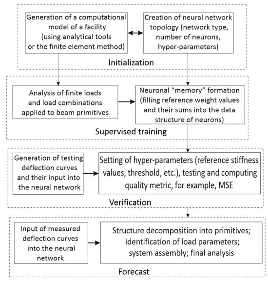
Figure 1.
Main stages of load identification in linear beam systems.
The prediction block is described in detail in Section 2.2. This principle can be used to design more complex systems that have beams and columns, such as multi-story frame structures of civil buildings. Other blocks of this scheme are described in Section 2.4 and Section 2.5.
2.2. General Provisions and Formulations for Steel Frame Systems
A steel bearing structure, subjected to 3D deformation, is considered in the article. The finite-element method is used to make a computational model of this structure. In the general case, the model may have spatial rod elements, plates, shells, and solid bodies. The structure belongs to the first class of the stress–strain state, which means that no plastic deformations are acceptable during its normal operation. Its structural behavior is assumed to be linear in the elastic stage. Stiffness values of structural elements simulated using rods or plates and shells are assumed to be constant.
The task is to identify the type of action (a mechanical force or pre-set displacement) that the strained system is subjected to. For clarity, let us consider the frame structures shown in Figure 2a,b.
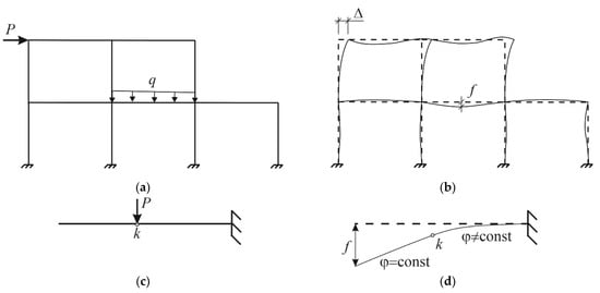
Figure 2.
Loads acting on frame systems. A frame and the load applied to it (a); a deformed scheme of the frame with peak deflections (b); a cantilever beam showing features of deflection (c); rotation angles in cross-sections of the beam segments (d).
Maximum deflections and arise when the frame is subjected to point force and linear load . These deflections predict the point of the force action. The curvature of the longitudinal axis is another indicator of the load application point. Using maximum deflection to identify the point of load without considering the curvature of the longitudinal axis can be erroneous, as illustrated in Figure 2c. Here, deflection is maximal at the point shown in Figure 2d, but the force is applied at a different point (k), and the longitudinal axis in the unloaded area remains undistorted (the rotation angle of cross-sections remains constant).
Types of actions that can be considered for identification purposes include a mechanical point force, linear uniformly distributed load, a concentrated bending moment, pre-set linear or angular displacement, etc. The type of action can be identified by considering both linear and angular displacements of nodes in a finite-element model. The size of the finite-element mesh also affects the accuracy of the action identification. Thus, Figure 3a–c shows structures having the same horizontal deflection , but also different loads that triggered this deflection. The figure shows that such loads can be identified by evaluating nodal displacements and rotation angles. Evidently, the accuracy of such an evaluation is determined using the number of nodes in which linear displacements and angular displacements are obtained.
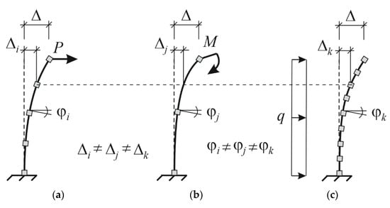
Figure 3.
Identification of actions for cases of identical deflection. : A post showing different cell sizes of a finite-element mesh and identical displacement of the top node loaded by the point force (a); the moment (b); distributed load (c).
Hence, making a pool of stress–strain states is a necessary and sufficient condition for the qualitative and quantitative identification of a type of mechanical action that a load-bearing structure is subjected to. These stress–strain states can correspond to conditions of normal operation and emergency actions. In the first case, for a steel structure of the first class of the stress–strain state, strength and stiffness constraints must be satisfied as follows:
where are equivalent stresses computed using the maximum strain energy theory postulated by von Mises; is the design resistance of structural steel, assigned using the yield strength value; is deflection of a structure triggered by an external load, is the deflection value (2) acceptable according to the aesthetic requirements and (3) depending on the span.
In case of an emergency action no stress limits should apply, because the task is to determine maximum deformations and deflections that help to identify the point of structural failure.
where , are the relative deformation and deflection of a structure as a result of an emergency situation, respectively; is the relative deformation corresponding to the temporary resistance (ultimate strength) of steel; is the deflection at which material assets and humans can be safely evacuated from a building.
Conditions (2) and (3) can be applied to predict the emergency-triggered behavior of a deformed structure subjected to displacements in the process of operation.
2.3. Decomposition of Beam Structures under Normal Operating Conditions
Most beam structures can be represented as a set of simple beams, including cantilevered rods, hinged beams without cantilevers, and hinged beams with cantilevers. Examples of complex systems, consisting of simple beams, are shown in Figure 4a.
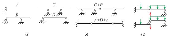
Figure 4.
Decomposition of beam systems into primitives for machine learning purposes: simple beams (primitives) (a); A–D types of primitives; types of composite beam systems (b); beam decomposition into two primitives (c).
Let us focus on the background of the identification methodology. Parameters of load, acting on a composite beam system, can be predicted using models trained on simple beams (the main types of beams are shown in Figure 4b). Hence, identification of loads, acting on an arbitrary system, requires a model that must be trained on the main types of simple beams subjected to different types of loads and actions. The case of decomposition with reaction transfer from one beam to another is shown in Figure 4c. The hinge reaction is highlighted in red. Similarly, floor and roof beams of frame structures can also be described using single-span beams with various kinematically constrained support nodes.
One of the main challenges accompanying the development of a neural network is the method of its training. Proven methods of training linear regression equations [,] for example, methods of stochastic gradient descent and many others, are not quite effective in the general case of composite structural systems. The reason for their poor effectiveness is a very large number of calculations must be made to ensure accurate deflection predictions and identification of loads for a complex system. The time frame, needed for a structural designer to make these calculations is unacceptable. Therefore, a procedure involving deflection curves in a cross-section subjected to a moving unit load serves as the basis for the training method to be used in the case under consideration. Deflections will serve as the source of sets of weights to be generated for training purposes. Input weights should be duly scaled to ensure their comparability with reference weights obtained during training. Scaling can be performed by setting as the reference value of the rod stiffness and using the following expression to adjust weights of the input signal :
where is the vector of scaled weights of the input signal, is the actual stiffness of the rod in tension–compression , in plane bending , [,], etc. Here, is the modulus of elasticity of the material; is the cross-sectional area; and is the moment of inertia relative to the bending axis.
2.4. Patterns of Emergency Situations
A sudden failure of one of the columns is the most dangerous and characteristic emergency situation for beam and frame structures. Such an emergency situation can be simulated by (1) developing individual scenarios of progressive collapse escalation prevention and (2) taking into account the nonlinear behavior of structural elements. The level of elastic deflections must first be determined for a system with a removed link. The elastic curve, conveying the stiffness of the system elements, must correspond to such elastic deflections. Further deformation of the system can be represented as a mechanism with conventional plastic hinges; this mechanism is in motion until it reaches the stage of ultimate deformations corresponding to initiation of material fracture.
2.5. Using Basic Cross-Sections of Simple Beams to Train the Neural Network
In the general case, each neuron, designated for storing the training information, must have an array of 6 real numbers, where 6 is the number of degrees of freedom of a finite-element model in a node. Therefore, the training matrix has size , where is the number of nodes used for training purposes. In a special case, for a 2D system. It is noteworthy that not all nodes will be subjected to large displacements triggered by the load application; support nodes will have zero displacements. That is why it is necessary to exclude them from the training set.
Let the load-bearing structure be subjected to actions represented by vector in the general case, where is the number of load combinations in the training set of load combinations that should not cause any disruption to normal operating conditions. A unit action (an action of a force or load, whose value equals one) is considered for neurons training purposes. Each action forms vector (2). A family of reference curves, plotted according to the structure of vector , can be described as a result of structural analysis made using the finite-element method or the analytical method. Let us represent this set of vectors as a training data array . Let us represent this array by describing each point of the curve with the help of weight coefficient :
where is a displacement vector component in some cross-section S; and are displacement components in other cross-sections. coefficients are unique for each curve. They describe its shape. Therefore, it is important to use all cross-sections of a structure to obtain the most detailed information about the nature of its deflection.
This family of curves can be used to make quadratic equations and higher-order polynomials in the general case. These polynomials are regression curves that make predictions in terms of load identification. Due to the continuity of deflection curves, values of components of displacement vectors determine mutual positions of nodes and can be interpreted as connections between neurons (nodes of a structure in the training set). When solid bodies are used to simulate structures, nodes must be located on the longitudinal axis or the median surface of these bodies. Since linearly deformed systems are considered, a deflection curve can be used to identify internal forces and stresses in a structure.
Cases of data generation using characteristic nodes of the training set are shown in Figure 5. It is noteworthy that in some cases the task of determining the stress state is difficult to accomplish. If a linearly deformed system is considered, then load identification and stress determination can require one characteristic point in cross-section , for which the linear displacement and the rotation angle (the curvature of an element) can be measured; see Figure 5a. If refined identification is needed for items subjected to complex resistance, several points can be used for a cross-section, such as four corner points ; see Figure 5b.
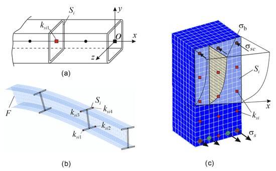
Figure 5.
Generation of data needed to train the neural network: a rod model (a); a model composed of plate or shell elements (b); a model composed of 3D and rod elements; are normal stresses in concrete, tensile and compressed rebars, respectively; F is a rigidly restrained edge, a 3D model of a reinforced concrete rod (c).
For these points, displacements in the cross-section plane and cross-sectional rotation angles can be measured to ensure a more accurate identification of load and the stress state. The features and complexity of this measurement method prevent it from being addressed in this article; the most widespread and simple examples are described in the Section 3. Figure 5c can serve as an example of future-oriented research efforts that focus on identifying characteristic points needed for training purposes. This figure shows a fragment of a 3D model of a reinforced concrete rod in a complex stress state. Four corner points are not sufficient in this case, because displacements of the cross-section, same as its size, depend on cracking and the crack opening width. However, 3D cracking may occur, and cracks can have different opening width and depth values, etc.
2.6. Load Identification Based on Evaluation of the Threshold Function Values
Let us consider load cases typical for steel building frames. They include (1) load uniformly distributed along the length of a rod and (2) a point force. The assumption is that distributed load is applied along the rod span. Hence, the load value and the indicator of the presence or absence of this load on the rod can serve as identification parameters, taking “0” and “1” values, respectively. The presence of load is associated with vector , where , and its absence is associated with deflection vector , corresponding to initial boundary conditions. As for the point force, its identification parameters can be represented as the following values: the force application point , which is a numerical identifier associated with the standardized shape of the deflection curve depending on the force applied to the rod cross-section considered here; is the actual value of this force. The characteristic of identification parameters is shown in Figure 6.
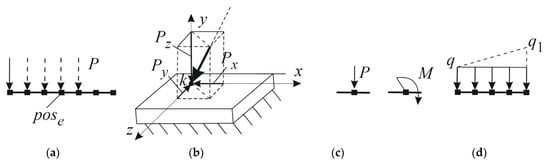
Figure 6.
Load identification parameters: application point (a), direction and value (b), type of point load (c), type of distributed load (d).
The following principles can be used to identify load parameters depending on the problem to be solved.
- -
- The absolute value of the difference between sums of weights of an input vector and a training vector for all cross-sections should not exceed the threshold (7). This dependence can apply to rods shown in Figure 5a; their displacement is identified for one degree of freedom only, and cross-sectional deformations satisfy the Bernoulli hypothesis:
- -
- The sum of squared deviations for all cross-sections and displacements, involved in the identification process, should not exceed the threshold (8). In general, it is used for 3D systems and cross-sections for which the Bernoulli hypothesis is satisfied.
- -
- For the sum of squared deviations for the considered cross-sections and all displacements involved in the identification process, for all characteristic points of cross-sections, should not exceed the threshold (9). This dependence is applied to 3D systems subjected to complex resistance, and cross-sections of elements may be subjected to warping, cracking, and other effects.
The threshold is a positive value selected depending on the dimension of the problem to be solved. In this case, a variable can be introduced:
The “+” sign of variable means that the parameter of the action is identified, e.g., the force application point is found; the emergency failure of the column is identified, etc.
3. Results
3.1. Identification of Point Force Parameters
A 2D scheme is considered as a special case: linear displacements in the directions of x, y axes and angular displacements r in the beam plane are possible for each of the cross-sections . Let us make a data structure of neurons associated with cross-sections . Each of them will have the following matrix:
Given that x, y, r displacement curves have no discontinuities and are unique, one layer of neurons will be sufficient to identify one type of load, as shown in Figure 7.
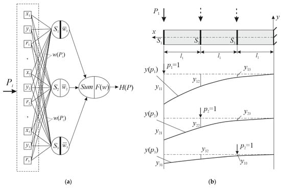
Figure 7.
Model training: the network topology (a) and stages of beam training using three cross-sections (b).
The point of application and the value of the point force can be identified using the existing deformation scheme: network topology generation, as shown in Figure 7. In this case, Expressions (3) and (6) are used to make arrays for neurons, and the summation unit is generated. This summation unit makes a prediction about the presence or absence of a point force in a cross-section on the basis of Expressions (7)–(10). At this stage, elements of matrices, made for the cross-sections on the basis of Expression (11), are empty.
Network training results in filling the bottom block of matrices (11) through obtaining the values of . This procedure is shown in Figure 7b. The total length of the beam and reference stiffness are set. Unit force is applied to each cross-section, and deflections are computed, where i is the number of the cross-section to which the force is applied; j is the number of the cross-section for which displacement is computed.
For the identification of the force application point and value, the vector of displacements triggered by a point force is measured, and the values of are computed using Expression (5). The sums of reference and measured weights are computed and directed to the summation unit. Further, Expression (10) is used to make a prediction. If it is equal to one, then the value of the actual force is computed as follows:
is the measured value of deflection in the cross-section in which the force application point is identified; this value is directed to the network; is the value of deflection triggered by force , acting in this cross-section. The values of limit state criteria can be refined using Formulas (1) and (2), if the value of is already computed.
3.2. Case 1: A Cantilever Beam
Let us identify the load acting on a cantilever beam, which is (1) under the action of some force and (2) in the strain state shown in Figure 8.
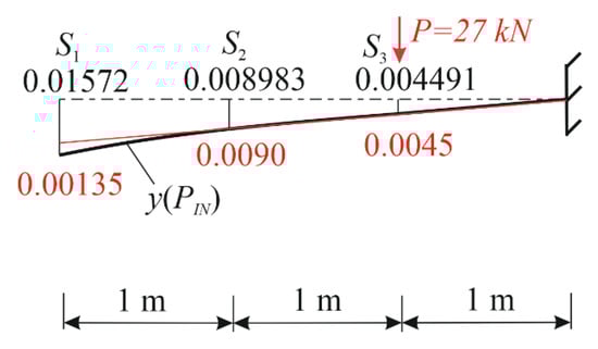
Figure 8.
Measured deflections and the result of the force identification.
The assumption is that it is impossible to (1) visually determine the force application point and (2) measure its value. The assumption is that all displacements , and rotation angles will be disregarded in this case. Measured values of deflections, interpreted as an input signal, are highlighted in black in Figure 8. To simplify the computations, let us assume that stiffness equals and that this value also equals the reference stiffness value used to train the neural network, then according to (4), .
The model is trained using three cross-sections at the points where deflections were measured. Displacements in the force application point will be found using a well-known formula obtained with the help of Moore’s integrals , assuming that , and is the distance from the fixed node to the force application point. In other cross-sections, displacements can be found using geometric similarity. Let force act in the cross-section at the cantilever edge, then , , . Then, weights of the resulting deflection curve are computed as follows: , ; . This procedure is reproduced for the second and third cross-sections. Training results can be presented as Expression (11):
The assignment of the threshold value needs an independent research undertaking; let us assume that the threshold value equals for this task, taking into account some error in the computation of displacements. Measured data (Figure 8) are taken to compute weights of the curve of measured deflections according to Formula (5) and to fill the top block of matrices :
Let us find the force application point:
Cross-section : no.
Cross-section : no.
Cross-section : yes. The force application point is located in the neighborhood of cross-section . The deflection triggered by the unit force in this cross-section m; according to Formula (12), its value equals kN.
It is noteworthy that this solution is approximate, and it strongly depends on the value of . If it were smaller by 0.0014 in this case (see the force application point search for cross-section ), then the force application point would not be identified in any of the cross-sections, because for each cross-section . In this case, a larger number of cross-sections would have to be considered for training purposes. Indeed, if a deflection curve is plotted for the case of force kN (see the value highlighted in red in Figure 8), there is a difference between deflection values in one of the cross-sections. This means that there is a need to introduce (1) an evaluation, based on rotation angles r, and (2) supplementary cross-sections, and there is also no need to re-train the neural network. Deviations in deflections may be caused by nonlinear effects, which are planned to be taken into account in further research works.
3.3. Case 2: A Hinged Beam
Let us identify parameters of a load, which can be distributed over the entire rod or applied to some node as a point load. In addition, let us demonstrate how load combinations can be identified. An initial beam and unique curves, illustrating different load types and application points, are shown in Figure 9.
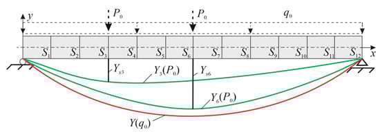
Figure 9.
A hinged beam showing cross-sections used for training purposes: are deflection curves triggered by a force located in cross-section ; is a deflection curve triggered by the load uniformly distributed along the entire length of the rod.
The span of the beam is 6 m; cross-sections are spaced at intervals of 0.5 m. Cross-sections will be interpreted as neurons. The rod is made of structural steel and has a W10 × 60 I-beam section. For training purposes, the force value equals 10 kN. The network topology is essentially the same as in Figure 7a.
3.4. Identification of the Point Force
Let us train the network. The finite-element method will be used to find deflections and reference weights in this problem. The matrix of displacements and their graphical interpretation are shown in Figure 10.
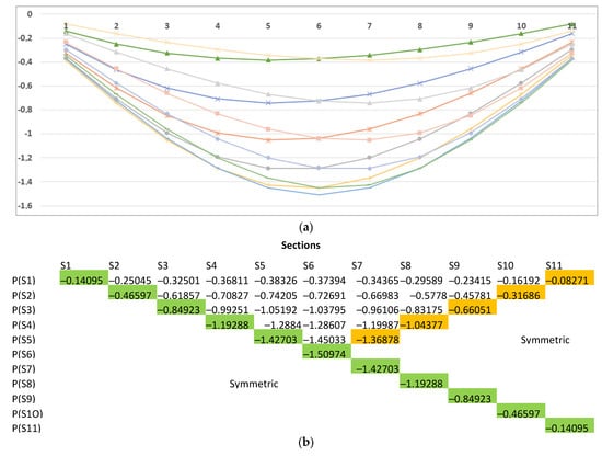
Figure 10.
Preparation for model training: deflection curves (a) and their matrix (b); S1–S11 are beam cross-sections; P(S1) is the force application point in these cross-sections. Colors highlight the elements of the main (green) and side (orange) diagonal in the matrix.
Let us use Expressions (4) and (5) to make a weight matrix for Expression (6) in respect of the vertical linear displacements.
| Neurons | |||||||||||
| N1 | N2 | N3 | N4 | N5 | N6 | N7 | N8 | N9 | N10 | N11 | |
| 1 | 0.56279 | 0.43368 | 0.3829 | 0.36777 | 0.37693 | 0.41016 | 0.47636 | 0.60196 | 0.87049 | 1.70417 | |
| 1.86053 | 1 | 0.7533 | 0.6579 | 0.62795 | 0.64103 | 0.69565 | 0.80646 | 1.01782 | 1.47059 | 2.87778 | |
| 2.61293 | 1.37289 | 1 | 0.85564 | 0.80731 | 0.81818 | 0.88364 | 1.02102 | 1.28572 | 1.85498 | 3.62686 | |
| 3.24055 | 1.68422 | 1.20188 | 1 | 0.92586 | 0.92754 | 0.99417 | 1.14286 | 1.43418 | 2.06452 | 4.0315 | |
| 1948265 | 1.92309 | 608496 | 1.1076 | 1 | 0.98393 | 1.04256 | 1.18932 | 1.48485 | 2.13044 | 4.15257 | |
| 4.03739 | 2.07693 | 1.45454 | 1.17392 | 1.04096 | 1 | 1.04096 | 1.17392 | 1.45454 | 2.07693 | 4.03739 | |
| 4.15257 | 2.13044 | 1.48485 | 1.18932 | 1.04256 | 0.98393 | 1 | 1.1076 | 608496 | 1.92309 | 1948265 | |
| 4.0315 | 2.06452 | 1.43418 | 1.14286 | 0.99417 | 0.92754 | 0.92586 | 1 | 1.20188 | 1.68422 | 3.24055 | |
| 3.62686 | 1.85498 | 1.28572 | 1.02102 | 0.88364 | 0.81818 | 0.80731 | 0.85564 | 1 | 1.37289 | 2.61293 | |
| 2.87778 | 1.47059 | 1.01782 | 0.80646 | 0.69565 | 0.64103 | 0.62795 | 0.6579 | 0.7533 | 1 | 1.86053 | |
| 1.70417 | 0.87049 | 0.60196 | 0.47636 | 0.41016 | 0.37693 | 0.36777 | 0.3829 | 0.43368 | 0.56279 | 1 | |
Now, let us apply input signal to the neural network. The input signal is applied in the form of measured deflections triggered by some point force whose position and value are unknown.
Let us fill the matrix of input signal weights using (4), and (5) for each element of this input vector. The resulting matrix is as follows:
| Neurons | |||||||||||
| N1 | N2 | N3 | N4 | N5 | N6 | N7 | N8 | N9 | N10 | N11 | |
| 1 | 0.520623 | 0.372685 | 0.311702 | 0.289903 | 0.291225 | 0.312702 | 0.359901 | 0.452004 | 0.651008 | 1.271613 | |
| 1.920776 | 1 | 0.715845 | 0.59871 | 0.556839 | 0.559379 | 0.60063 | 0.691289 | 0.868199 | 1.25044 | 2.442483 | |
| 2.683228 | 1.39695 | 1 | 0.836367 | 0.777877 | 0.781424 | 0.83905 | 0.965696 | 1.21283 | 1.746802 | 3.412027 | |
| 3.208193 | 1.670258 | 1.195647 | 1 | 0.930066 | 0.934307 | 1.003207 | 1.154632 | 1.450117 | 2.088557 | 4.079578 | |
| 3.449426 | 1.79585 | 1.285551 | 1.075193 | 1 | 1.004561 | 1.078641 | 1.241452 | 1.559155 | 2.245602 | 4.386333 | |
| 3.433765 | 1.787697 | 1.279714 | 1.070311 | 0.99546 | 1 | 1.073744 | 1.235815 | 1.552076 | 2.235407 | 4.366419 | |
| 3.197936 | 1.664919 | 1.191824 | 0.996803 | 0.927092 | 0.931321 | 1 | 1.15094 | 1.445481 | 2.081881 | 4.066537 | |
| 2.778542 | 1.446572 | 1.035522 | 0.866077 | 0.805509 | 0.809182 | 0.868855 | 1 | 1.255913 | 1.808852 | 3.533229 | |
| 2.212369 | 1.15181 | 0.824518 | 0.6896 | 0.641373 | 0.644298 | 0.691811 | 0.796234 | 1 | 1.440269 | 2.813276 | |
| 1.536081 | 0.799719 | 0.572475 | 0.478799 | 0.445315 | 0.447346 | 0.480335 | 0.552837 | 0.694315 | 1 | 1.953299 | |
| 0.786403 | 0.409419 | 0.293081 | 0.245123 | 0.227981 | 0.229021 | 0.24591 | 0.283027 | 0.355457 | 0.511954 | 1 | |
The threshold = 0.01 is set to compute deviations for each cross-section and the threshold function value: ; computation results are shown in Table 1. A positive identification result for cross-section means that the model predicts the point of application of some point force in this cross-section. The table shows that it is cross-section .

Table 1.
Identification of the force application point.
Since the force is located in cross-section , in the case of linear deformation, its value can be predicted using the ratio of input and reference deflections (see the matrix in Figure 10b and input vector ):
kN. The input vector was obtained when the value of vertical force was kN; the force was applied 10 cm to the left of the cross-section . If the prediction is compared with the exact solution, it can be argued that this discretization of a structure into cross-sections can be applied to achieve high prediction accuracy.
3.5. Identification of the Distributed Load
Another layer of neurons is needed, because a new type of load is addressed here, and the model is not trained in it. The structure of these neurons is the same as that required for the point force identification. The distributed load q = 10 kN/m will be applied to the system (Figure 9) to have a vector of training displacements generated. These training displacements will be used to compute weights in cross-sections –. These displacements can be accurately computed using Moore’s integrals, or the finite-element method can be applied. In the latter case, each node of the model will be associated with cross-sections . The result is shown in Figure 11.
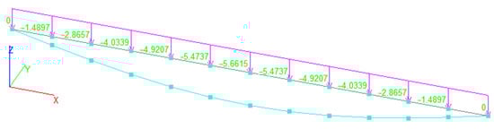
Figure 11.
Using the finite-element method to obtain matrix coefficients : numbers indicate deflections used for training purposes.
The matrix of weight coefficients, stored in the memory of neurons, will be constructed on the basis of the assumption that the load, uniformly distributed along the length, is applied to each cross-section. If the force application point is in the cross-section, one row vector can be sufficiently created by performing its normalization using the value of displacement in the cross-section to which the force is applied. However, 11 vectors are created in this case. Their normalization is performed using the value of displacement in the cross-section. Given that the load is uniformly distributed in all beam cross-sections, the result will be as follows:
| Matrix | |||||||||||
| N1 | N2 | N3 | N4 | N5 | N6 | N7 | N8 | N9 | N10 | N11 | |
| 1 | 0.519838 | 0.369295 | 0.302741 | 0.272156 | 0.263128 | 0.272156 | 0.302741 | 0.369295 | 0.519838 | 1 | |
| 1.923676 | 1 | 0.710404 | 0.582376 | 0.52354 | 0.506173 | 0.52354 | 0.582376 | 0.710404 | 1 | 1.923676 | |
| 2.707861 | 1.407649 | 1 | 0.819782 | 0.73696 | 0.712514 | 0.73696 | 0.819782 | 1 | 1.407649 | 2.707861 | |
| 3.303148 | 1.717102 | 1.219837 | 1 | 0.898971 | 0.869151 | 0.898971 | 1 | 1.219837 | 1.717102 | 3.303148 | |
| 3.674364 | 1.910074 | 1.356925 | 1.112382 | 1 | 0.966829 | 1 | 1.112382 | 1.356925 | 1.910074 | 3.674364 | |
| 3.80043 | 1.975608 | 1.403481 | 1.150548 | 1.03431 | 1 | 1.03431 | 1.150548 | 1.403481 | 1.975608 | 3.80043 | |
| 3.674364 | 1.910074 | 1.356925 | 1.112382 | 1 | 0.966829 | 1 | 1.112382 | 1.356925 | 1.910074 | 3.674364 | |
| 3.303148 | 1.717102 | 1.219837 | 1 | 0.898971 | 0.869151 | 0.898971 | 1 | 1.219837 | 1.717102 | 3.303148 | |
| 2.707861 | 1.407649 | 1 | 0.819782 | 0.73696 | 0.712514 | 0.73696 | 0.819782 | 1 | 1.407649 | 2.707861 | |
| 1.923676 | 1 | 0.710404 | 0.582376 | 0.52354 | 0.506173 | 0.52354 | 0.582376 | 0.710404 | 1 | 1.923676 | |
| 1 | 0.519838 | 0.369295 | 0.302741 | 0.272156 | 0.263128 | 0.272156 | 0.302741 | 0.369295 | 0.519838 | 1 | |
Now let us set input vectors (for example, actual measured deflections) and focus on the process of identifying a uniformly distributed load and its value. Let us set three vectors presented in Table 2. A finite-element model shown in Figure 11 is used to generate these vectors. Load parameters will not be demonstrated to illustrate the correctness of identification parameters.
Table 2.
Input displacement vectors .
Formula (5) is used, since the load application point is already known and the main task is to determine its type. Let us make matrices for actions .
| Matrix | |||||||||||
| 1 | 0.51442 | 0.36027 | 0.29076 | 0.25783 | 0.24769 | 0.25783 | 0.29076 | 0.36027 | 0.51442 | 1 | |
| 1.94393 | 1 | 0.70034 | 0.56522 | 0.50121 | 0.48148 | 0.50121 | 0.56522 | 0.70034 | 1 | 1.94393 | |
| 2139259 | 1.42789 | 1 | 0.80707 | 0.71567 | 0.6875 | 0.71567 | 0.80707 | 1 | 1.42789 | 2.7757 | |
| 3.43924 | 1.76923 | 1.23905 | 1 | 0.88675 | 0.85185 | 0.88675 | 1 | 1.23905 | 1.76923 | 3.43924 | |
| 3.87848 | 1.99518 | 757150 | 1.12771 | 1 | 0.96065 | 1 | 1.12771 | 757150 | 1.99518 | 3.87848 | |
| 4.03737 | 2.07691 | 1.45454 | 1.17391 | 1.04096 | 1 | 1.04096 | 1.17391 | 1.45454 | 2.07691 | 4.03737 | |
| 3.87848 | 1.99518 | 757150 | 1.12771 | 1 | 0.96065 | 1 | 1.12771 | 757150 | 1.99518 | 3.87848 | |
| 3.43924 | 1.76923 | 1.23905 | 1 | 0.88675 | 0.85185 | 0.88675 | 1 | 1.23905 | 1.76923 | 3.43924 | |
| 2139259 | 1.42789 | 1 | 0.80707 | 0.71567 | 0.6875 | 0.71567 | 0.80707 | 1 | 1.42789 | 2.7757 | |
| 1.94393 | 1 | 0.70034 | 0.56522 | 0.50121 | 0.48148 | 0.50121 | 0.56522 | 0.70034 | 1 | 1.94393 | |
| 1 | 0.51442 | 0.36027 | 0.29076 | 0.25783 | 0.24769 | 0.25783 | 0.29076 | 0.36027 | 0.51442 | 1 | |
| Matrix | |||||||||||
| 1 | 0.52588 | 0.38033 | 0.31919 | 0.29521 | 0.29475 | 0.31518 | 0.36174 | 0.45347 | 0.65232 | 1.27334 | |
| 1.90157 | 1 | 0.72322 | 0.60695 | 0.56136 | 0.5605 | 0.59934 | 0.68788 | 0.8623 | 1.24044 | 2.42134 | |
| 2.62931 | 1.38271 | 1 | 0.83924 | 0.7762 | 0.775 | 0.82871 | 0.95114 | 1.19231 | 1.71516 | 3.348 | |
| 3.13297 | 1.64757 | 1.19155 | 1 | 0.92488 | 0.92346 | 0.98746 | 1.13333 | 842616 | 2.04371 | 3.98932 | |
| 3.38742 | 1.78138 | 1.28833 | 1.08122 | 1 | 0.99846 | 1.06766 | 1.22538 | 1.53609 | 2.20969 | 4.31333 | |
| 3.39265 | 1.78413 | 1.29032 | 1.08289 | 1.00154 | 1 | 1.0693 | 1.22727 | 1.53846 | 84404 | 4.31998 | |
| 3.17277 | 1.74768 | 1.20669 | 1.0127 | 0.93663 | 0.93519 | 1 | 1.14773 | 1.43875 | 2.06967 | 4.5386 | |
| 2.76439 | 1.45374 | 1.05137 | 0.88235 | 0.81608 | 0.81482 | 0.87129 | 1 | 1.25356 | 1.80328 | 1.9054 | |
| 2.20523 | 1.15969 | 0.83871 | 0.70388 | 0.65101 | 0.65 | 0.69505 | 0.79773 | 1 | 1.43852 | 2.808 | |
| 1.53298 | 0.80617 | 0.58304 | 0.48931 | 0.45255 | 0.45185 | 0.48317 | 0.55455 | 0.69516 | 1 | 1.952 | |
| 0.78534 | 0.413 | 0.29869 | 0.25067 | 0.23184 | 0.23148 | 0.24752 | 0.28409 | 0.35613 | 0.51229 | 1 | |
| Matrix | |||||||||||
| 1 | 0.51982 | 0.36929 | 0.30274 | 0.27215 | 0.26312 | 0.27215 | 0.30274 | 0.36929 | 0.51982 | 1 | |
| 1.92375 | 1 | 0.71042 | 0.58239 | 0.52354 | 0.50617 | 0.52354 | 0.58239 | 0.71042 | 1 | 1.92375 | |
| 2.70791 | 1.40762 | 1 | 0.81978 | 0.73695 | 0.7125 | 0.73695 | 0.81978 | 1 | 1.40762 | 2.70791 | |
| 3.30321 | 1.71707 | 1.21984 | 1 | 0.89896 | 0.86913 | 0.89896 | 1 | 1.21984 | 1.71707 | 3.30321 | |
| 3.67449 | 1.91006 | 1.35695 | 1.1124 | 1 | 0.96682 | 1 | 1.1124 | 1.35695 | 1.91006 | 3.67449 | |
| 3.80058 | 1.97561 | 1.40351 | 1.15057 | 1.03432 | 1 | 1.03432 | 1.15057 | 1.40351 | 1.97561 | 3.80058 | |
| 3.67449 | 1.91006 | 1.35695 | 1.1124 | 1 | 0.96682 | 1 | 1.1124 | 1.35695 | 1.91006 | 3.67449 | |
| 3.30321 | 1.71707 | 1.21984 | 1 | 0.89896 | 0.86913 | 0.89896 | 1 | 1.21984 | 1.71707 | 3.30321 | |
| 2.70791 | 1.40762 | 1 | 0.81978 | 0.73695 | 0.7125 | 0.73695 | 0.81978 | 1 | 1.40762 | 2.70791 | |
| 1.92375 | 1 | 0.71042 | 0.58239 | 0.52354 | 0.50617 | 0.52354 | 0.58239 | 0.71042 | 1 | 1.92375 | |
| 1 | 0.51982 | 0.36929 | 0.30274 | 0.27215 | 0.26312 | 0.27215 | 0.30274 | 0.36929 | 0.51982 | 1 | |
The appearance of primary and secondary diagonals of matrix proves that action does not correspond to the symmetrical shape of the deflection curve, so it can be excluded from any detailed consideration. If the rod is subjected to a symmetrical distributed load, the deviation of action weights and the reference curve will tend to zero within the rounding accuracy; that is why we set a sufficiently small threshold of = 0.0001. Then, computations are made using Formula (9), Table 3.
Table 3.
Identification of actions and .
According to Table 3, action is unambiguously identified as a uniform load acting on the rod. Its value will be as follows for a linear system (see Table 2 and Figure 11):
t/m =29.999 kN/m
Figure 12 shows actions that caused the deflections are provided to illustrate the accuracy of identification.
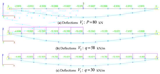
Figure 12.
Beams featuring deflections and loads considered for identification purposes: a curve describing the point force (a); a curve describing the point load (b) and the load distributed over the entire span (c); yellow frames – constrained nodes.
4. Discussion and Areas of Further Research
The proposed identification method can be applied to other types of steel structures, such as frames, by adapting training procedures to convey the characteristic properties of these structures (geometry, types of nodal connections, and the nature of loads acting on them). The algorithm presented in the article allows the prediction of load parameters only for those types of loads and primitives that were considered in the course of training. If a structure can be composed of primitives as shown in Figure 4, the identification of parameters for loads of the same type does not cause any difficulties. However, if a combination of loads is considered, the proposed algorithm cannot generate any adequate prediction results without a prior adaptation. If it is necessary to identify load parameters or a combination of loads for complex 3D systems, the following adaptation should be performed:
- − reproduce the boundary conditions for each primitive within a complex system;
- − develop a load superposition algorithm;
- − decompose the input displacement vector and search for further loads or load combinations, assuming that one of the loads is identified correctly.
Furthermore, an important area of research is the consideration of the physically and geometrically nonlinear behavior of a structure. However, this process may require a complex topology of a neural network with multiple hidden layers.
Further research can be made into the number of cross-sections needed for training purposes, the mathematical substantiation of the threshold value, the examination of prediction effectiveness using models with different levels of detail (LOD), etc.
The evaluation of performance metrics, such as the accuracy, precision, and recall of machine learning models, is a vital issue []. This evaluation and further adjustment of these metrics can strongly affect the prediction result. In the general case, a comprehensive set of metrics is needed if no analytic expressions can be made to find the weight coefficients. In this case, heuristic optimization methods are used. No advanced analysis of prediction accuracy is needed in this work due to the small spread and range of data in the training dataset.
However, many tasks require solving important issues such as preparing and selecting data for the training dataset, choosing the model validation method, evaluating the data spread [], making model ensembles and tuning their interaction, etc.
The need for a specific task of identifying loads acting on steel structures stems from tasks (1) about additional displacements detected in the course of monitoring the stress–strain state of power line supports, and (2) about causes of roof truss emergencies to be identified. Examples of these structures are shown in Figure 13.
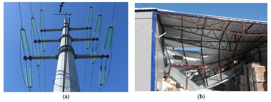
Figure 13.
Cases of load identification by displacements: power line supports (a); roof trusses after an accident (b), f is the deviation of displacements caused by the uncertain load; f -upper point deflection.
It should be noted that solving these tasks without the use of machine learning is possible but quite difficult. Machine learning elements are a highly effective way to address these problems. Moreover, a database of beam and column structures can be created to make predictions for various frame systems. This database can be applied to evaluate loads by deflection curves plotted for steel, concrete, reinforced concrete, and other composite structures. This approach can have a great future if applied to predict the effectiveness of strengthening damaged structures.
5. Conclusions
The research presented in this article achieved two main goals. The first is the ability to identify load parameters that cannot be directly determined, which enhances the reliability of steel structures and allows for forecasting the degree of hazard these loads pose to the structure. The second goal is the ability to determine the actual causes of deformations, including emergency impacts, if they are caused by loads that are no longer acting or whose intensity is difficult to measure.
The main results are as follows:
(1) The concept of load identification is proposed for linear steel frame systems. This concept is based on decomposition of a system into primitives (simple rods). Primitives are used for machine learning purposes within the framework of this concept. The purpose of machine learning is to identify the type, the point of application, and the value of loads;
(2) Analogies of neural network technologies are applied to develop a procedure for identifying the type of load, including point forces and longitudinal loads acting along the beam length;
(3) Primitives, such as cantilever beams and hinged single-span beams, are used to develop a procedure for identifying the force value and point of application, the presence, the absence and the value of a longitudinal load distributed along the entire length of a rod;
(4) Analytic expressions, developed to evaluate the identification accuracy using formulas proposed for evaluating the model quality, show that approaches to the prediction of loads and their parameters are efficient and quite accurate.
These findings can be contributed to computer-aided engineering systems used to inspect load-bearing structures, to evaluate their stress–strain properties and loading level, and to identify loads if their direct identification is impossible or points of application cannot be accurately determined.
Author Contributions
Conceptualization, A.R.T.; Methodology, A.V.A.; Software, A.V.A.; Validation, A.V.A. and O.A.T.; Formal analysis, A.V.A.; Investigation, A.V.A. and O.A.T.; Data curation, O.A.T.; Writing—original draft, A.V.A.; Writing—review & editing, O.A.T.; Visualization, O.A.T.; Supervision, A.R.T.; Project administration, A.R.T.; Funding acquisition, A.R.T. All authors have read and agreed to the published version of the manuscript.
Funding
The research was funded by the National Research Moscow State University of Civil Engineering (grant for fundamental and applied scientific research, project No. 04-234/130).
Data Availability Statement
The original contributions presented in the study are included in the article, further inquiries can be directed to the corresponding author.
Conflicts of Interest
The authors declare no conflict of interest.
References
- Jiao, P.; Roy, M.; Barri, K.; Zhu, R.; Ray, I.; Alavi, A.H. High-Performance Fiber Reinforced Concrete as a Repairing Material to Normal Concrete Structures: Experiments, Numerical Simulations and a Machine Learning-Based Prediction Model. Constr. Build. Mater. 2019, 223, 1167–1181. [Google Scholar] [CrossRef]
- Kumar, A.; Arora, H.C.; Mohammed, M.A.; Kumar, K.; Nedoma, J. An Optimized Neuro-Bee Algorithm Approach to Predict the FRP-Concrete Bond Strength of RC Beams. IEEE Access 2022, 10, 3790–3806. [Google Scholar] [CrossRef]
- Kumar, A.; Arora, H.C.; Kumar, K.; Mohammed, M.A.; Majumdar, A.; Khamaksorn, A.; Thinnukool, O. Prediction of FRCM–Concrete Bond Strength with Machine Learning Approach. Sustainability 2022, 14, 845. [Google Scholar] [CrossRef]
- Chen, S.Z.; Feng, D.C.; Han, W.S.; Wu, G. Development of Data-Driven Prediction Model for CFRP-Steel Bond Strength by Implementing Ensemble Learning Algorithms. Constr. Build. Mater. 2021, 303, 124470. [Google Scholar] [CrossRef]
- Aravind, N.; Nagajothi, S.; Elavenil, S. Machine Learning Model for Predicting the Crack Detection and Pattern Recognition of Geopolymer Concrete Beams. Constr. Build. Mater. 2021, 297, 123785. [Google Scholar] [CrossRef]
- Zhao, W.; Chen, F.; Huang, H.; Li, D.; Cheng, W. A New Steel Defect Detection Algorithm Based on Deep Learning. Comput. Intell. Neurosci. 2021, 2021, 5592878. [Google Scholar] [CrossRef] [PubMed]
- Naresh, M.; Kumar, V.; Pal, J. A Machine Learning Approach for Health Monitoring of a Steel Frame Structure Using Statistical Features of Vibration Data. Asian J. Civil. Eng. 2023, 25, 39–49. [Google Scholar] [CrossRef]
- Pal, J.; Sikdar, S.; Banerjee, S.; Banerji, P. A Combined Machine Learning and Model Updating Method for Autonomous Monitoring of Bolted Connections in Steel Frame Structures Using Vibration Data. Appl. Sci. 2022, 12, 11107. [Google Scholar] [CrossRef]
- Svendsen, B.T.; Øiseth, O.; Frøseth, G.T.; Rønnquist, A. A Hybrid Structural Health Monitoring Approach for Damage Detection in Steel Bridges under Simulated Environmental Conditions Using Numerical and Experimental Data. Struct. Health Monit. 2023, 22, 540–561. [Google Scholar] [CrossRef]
- Liu, Z.; Yuan, C.; Sun, Z.; Cao, C. Digital Twins-Based Impact Response Prediction of Prestressed Steel Structure. Sensors 2022, 22, 1647. [Google Scholar] [CrossRef]
- Naresh, M.; Sikdar, S.; Pal, J. Vibration Data-Driven Machine Learning Architecture for Structural Health Monitoring of Steel Frame Structures. Strain 2023, 59, e12439. [Google Scholar] [CrossRef]
- Perry, B.J.; Guo, Y.; Mahmoud, H.N. Automated Site-Specific Assessment of Steel Structures through Integrating Machine Learning and Fracture Mechanics. Autom. Constr. 2022, 133, 104022. [Google Scholar] [CrossRef]
- Yu, Y.; Wang, C.; Gu, X.; Li, J. A Novel Deep Learning-Based Method for Damage Identification of Smart Building Structures. Struct. Health Monit. 2019, 18, 143–163. [Google Scholar] [CrossRef]
- Nazarian, E.; Taylor, T.; Weifeng, T.; Ansari, F. Machine-Learning-Based Approach for Post Event Assessment of Damage in a Turn-of-the-Century Building Structure. J. Civ. Struct. Health Monit. 2018, 8, 237–251. [Google Scholar] [CrossRef]
- Rafiei, M.H.; Adeli, H. A Novel Machine Learning-Based Algorithm to Detect Damage in High-Rise Building Structures. Struct. Des. Tall Spec. Build. 2017, 26, e1400. [Google Scholar] [CrossRef]
- Gomez-Cabrera, A.; Escamilla-Ambrosio, P.J. Review of Machine-Learning Techniques Applied to Structural Health Monitoring Systems for Building and Bridge Structures. Appl. Sci. 2022, 12, 10754. [Google Scholar] [CrossRef]
- Gravett, D.Z.; Mourlas, C.; Taljaard, V.L.; Bakas, N.; Markou, G.; Papadrakakis, M. New Fundamental Period Formulae for Soil-Reinforced Concrete Structures Interaction Using Machine Learning Algorithms and ANNs. Soil Dyn. Earthq. Eng. 2021, 144, 106656. [Google Scholar] [CrossRef]
- Kazemi, F.; Asgarkhani, N.; Jankowski, R. Machine Learning-Based Seismic Fragility and Seismic Vulnerability Assessment of Reinforced Concrete Structures. Soil Dyn. Earthq. Eng. 2023, 166, 107761. [Google Scholar] [CrossRef]
- Xu, Y.; Li, Y.; Zheng, X.; Zheng, X.; Zhang, Q. Computer-Vision and Machine-Learning-Based Seismic Damage Assessment of Reinforced Concrete Structures. Buildings 2023, 13, 1258. [Google Scholar] [CrossRef]
- Wang, S.; Cheng, X.; Li, Y.; Song, X.; Guo, R.; Zhang, H.; Liang, Z. Rapid Visual Simulation of the Progressive Collapse of Regular Reinforced Concrete Frame Structures Based on Machine Learning and Physics Engine. Eng. Struct. 2023, 286, 116129. [Google Scholar] [CrossRef]
- Soh, M.F.; Bigras, D.; Barbeau, D.; Doré, S.; Forgues, D. Bim Machine Learning and Design Rules to Improve the Assembly Time in Steel Construction Projects. Sustainability 2022, 14, 288. [Google Scholar] [CrossRef]
- Zhao, Y.; Wang, N.; Liu, Z.; Mu, E. Construction Theory for a Building Intelligent Operation and Maintenance System Based on Digital Twins and Machine Learning. Buildings 2022, 12, 87. [Google Scholar] [CrossRef]
- Liu, Z.; Wu, D.; Liu, Y.; Han, Z.; Lun, L.; Gao, J.; Jin, G.; Cao, G. Accuracy Analyses and Model Comparison of Machine Learning Adopted in Building Energy Consumption Prediction. Energy Explor. Exploit. 2019, 37, 1426–1451. [Google Scholar] [CrossRef]
- Pomponi, F.; Anguita, M.L.; Lange, M.; D’Amico, B.; Hart, E. Enhancing the Practicality of Tools to Estimate the Whole Life Embodied Carbon of Building Structures via Machine Learning Models. Front. Built Environ. 2021, 7, 745598. [Google Scholar] [CrossRef]
- Alekseytsev, A.V.; Nadirov, S.H. Scheduling Optimization Using an Adapted Genetic Algorithm with Due Regard for Random Project Interruptions. Buildings 2022, 12, 2051. [Google Scholar] [CrossRef]
- Alekseytsev, A.V.; Al Ali, M. Optimization of Hybrid I-Beams Using Modified Particle Swarm Method. Mag. Civ. Eng. 2018, 83, 175–185. [Google Scholar] [CrossRef]
- Tusnina, O.; Alekseytsev, A. LOD of a Computational Numerical Model for Evaluating the Mechanical Safety of Steel Structures. Buildings 2023, 13, 1941. [Google Scholar] [CrossRef]
- Nilsen, M.; Bohne, R.A. Evaluation of BIM Based LCA in Early Design Phase (Low LOD) of Buildings. In Proceedings of the IOP Conference Series: Earth and Environmental Science, Xiamen, China, 7–9 June 2019; Volume 323. [Google Scholar]
- Dwairi, H.M.; Tarawneh, A.N. Artificial Neural Networks Prediction of Inelastic Displacement Demands for Structures Built on Soft Soils. Innov. Infrastruct. Solut. 2022, 7, 4. [Google Scholar] [CrossRef]
- Duan, X. Research on Prediction of Slope Displacement Based on a Weighted Combination Forecasting Model. Results Eng. 2023, 18, 101013. [Google Scholar] [CrossRef]
- Ma, J.; Xia, D.; Guo, H.; Wang, Y.; Niu, X.; Liu, Z.; Jiang, S. Metaheuristic-Based Support Vector Regression for Landslide Displacement Prediction: A Comparative Study. Landslides 2022, 19, 2489–2511. [Google Scholar] [CrossRef]
- Zhang, Y.; Tang, J.; Cheng, Y.; Huang, L.; Guo, F.; Yin, X.; Li, N. Prediction of Landslide Displacement with Dynamic Features Using Intelligent Approaches. Int. J. Min. Sci. Technol. 2022, 32, 539–549. [Google Scholar] [CrossRef]
- Yamazaki, Y.; Sakata, H. Simplified Prediction Method of Displacement Mode for Two-Story Wooden Structure with Eccentricity. J. Struct. Constr. Eng. 2018, 83, 467–477. [Google Scholar] [CrossRef][Green Version]
- Ye, Z.; Hsu, S.C. Predicting Real-Time Deformation of Structure in Fire Using Machine Learning with CFD and FEM. Autom. Constr. 2022, 143, 104574. [Google Scholar] [CrossRef]
- Asad, A.T.; Kim, B.; Cho, S.; Sim, S.H. Prediction Model for Long-Term Bridge Bearing Displacement Using Artificial Neural Network and Bayesian Optimization. Struct. Control Health Monit. 2023, 2023, 6664981. [Google Scholar] [CrossRef]
- Asgarkhani, N.; Kazemi, F.; Jakubczyk-Gałczyńska, A.; Mohebi, B.; Jankowski, R. Seismic Response and Performance Prediction of Steel Buckling-Restrained Braced Frames Using Machine-Learning Methods. Eng. Appl. Artif. Intell. 2024, 128, 107388. [Google Scholar] [CrossRef]
- Kazemi, F.; Jankowski, R. Machine Learning-Based Prediction of Seismic Limit-State Capacity of Steel Moment-Resisting Frames Considering Soil-Structure Interaction. Comput. Struct. 2023, 274, 106886. [Google Scholar] [CrossRef]
- Momeni, M.; Hadianfard, M.A.; Bedon, C.; Baghlani, A. Damage Evaluation of H-Section Steel Columns under Impulsive Blast Loads via Gene Expression Programming. Eng. Struct. 2020, 219, 110909. [Google Scholar] [CrossRef]
- Momeni, M.; Bedon, C.; Hadianfard, M.A. Probabilistic Evaluation of Steel Column Damage under Blast Loading via Simulation Reliability Methods and Gene Expression Programming. Eng. Proc. 2023, 53, 20. [Google Scholar] [CrossRef]
- Hittawe, M.M.; Langodan, S.; Beya, O.; Hoteit, I.; Knio, O. Efficient SST Prediction in the Red Sea Using Hybrid Deep Learning-Based Approach. In Proceedings of the IEEE International Conference on Industrial Informatics (INDIN), Perth, Australia, 25–28 July 2022; pp. 107–117. [Google Scholar]
- Harrou FZeroual, A.; Hittawe, M.M.; Sun, Y. Road Traffic Modeling and Management; Elsevier: Amsterdam, The Netherlands, 2022. [Google Scholar] [CrossRef]
- Hittawe, M.M.; Sidibé, D.; Mériaudeau, F. A Machine Vision Based Approach for Timber Knots Detection. In Proceedings of the Twelfth International Conference on Quality Control by Artificial Vision 2015, Le Creusot, France, 3–5 June 2015; Volume 9534. [Google Scholar]
- Hittawe, M.M.; Sidibé, D.; Beya, O.; Mériaudeau, F. Machine Vision for Timber Grading Singularities Detection and Applications. J. Electron. Imaging 2017, 26, 063015. [Google Scholar] [CrossRef]
- Shafighfard, T.; Kazemi, F.; Bagherzadeh, F.; Mieloszyk, M.; Yoo, D.-Y. Chained Machine Learning Model for Predicting Load Capacity and Ductility of Steel Fiber-Reinforced Concrete Beams. Comput.-Aided Civ. Infrastruct. Eng. 2024. [Google Scholar] [CrossRef]
- Chen, J.; Xiong, H.; Ventura, C.E. Seismic Reliability Evaluation of a Tall Concrete-Timber Hybrid Structural System. Struct. Des. Tall Spec. Build. 2022, 31, e1933. [Google Scholar] [CrossRef]
Disclaimer/Publisher’s Note: The statements, opinions and data contained in all publications are solely those of the individual author(s) and contributor(s) and not of MDPI and/or the editor(s). MDPI and/or the editor(s) disclaim responsibility for any injury to people or property resulting from any ideas, methods, instructions or products referred to in the content. |
© 2024 by the authors. Licensee MDPI, Basel, Switzerland. This article is an open access article distributed under the terms and conditions of the Creative Commons Attribution (CC BY) license (https://creativecommons.org/licenses/by/4.0/).