Experimental and Numerical Investigations of Mixing Performance of Mixing Agitators of Deep Cement Mixing Ships

Abstract

Recent decades have witnessed the increasing usage of deep cement mixing (DCM) mixers in the field of marine infrastructure construction. The mixing performance, including the torque history, can be helpful for structural safety evaluation, design, and the optimization of agitators, which is of engineering significance. However, to the best of the authors’ knowledge, there are no related publications that have reported the mixing behaviors of deep cement mixing agitators. In light of this, the present work conducts experimental and numerical investigations of the mixing behaviors of a DCM ship mixing agitator. To achieve this end, a model test device is established, and mixing experiments using two- and three-blade mixers are respectively conducted. Silt and clay soils are considered in the experiments with a three-blade mixer, while clay soils are used for those with a two-blade mixer. In addition, this work designs a torque transducer placed inside the rotating rod to accurately measure the torque history of the agitator during model test experiments. The experimental results show that, when mixing clay using agitators with different blades, the average torque value required for a two-blade agitator is slightly larger than that for a three-blade one. This study also presents a computational framework based on the arbitrary Lagrangian–Eulerian (ALE) method for an efficient and accurate modeling of the soil-mixing behaviors of the agitator. The numerical results are found to be in good agreement with the experimental data from model tests in terms of torque history, which demonstrates the effectiveness and capacity of our presented computational framework. The numerical results show that the average torque value is smaller at a higher rotational speed during the mixing of clay using a two-bladed agitator, but the effect of rotational speed on the torque history is small. The experimental and numerical methods introduced in the present work can act as a useful tool for investigations of mixing behaviors of DCM agitators.

1. Introduction

With the development of marine infrastructure construction, there is an increasing demand for advanced construction equipment. In marine infrastructure construction, soft foundation improvement has been a key issue. For the improvement and reinforcement of soft foundation problems, so-called deep cement mixing (DCM) technology [1] has found successful and widespread applications. Therefore, DCM ships have attracted a lot of attention among advanced marine equipment. However, a deep cement mixing ship faces a complex and changeable construction environment in practice, which is a big test for the performance of the main components of the DCM ship, such as the mixing agitator. Figure 1 shows a schematic diagram of a DCM ship. At present, most of the research on DCM technology focus on the quality of pile formation [2,3,4] and the bearing capacity of the improved soft foundation [5,6]. To the best of the authors’ knowledge, there are no existing publications that have studied the mixing behaviors of agitators. Therefore, this work introduces experimental and numerical approaches for investigating the torque behaviors of mixing agitators of a DCM ship, which is important for structural safety evaluation, design, and the optimization of the mixing head.

Conducting in situ testing of DCM marine mixer agitators is a major challenge due to the difficulty in establishing experimental set-ups, and the high cost. In contrast, model test experiments can be a good candidate for investigating the mixing behaviors of DCM mixing agitators. The model test results can be helpful in identifying soil types and predicting the mixing performance of agitators during in situ construction. On the other hand, numerical simulations have proved to be an efficient and effective tool to reproduce physical phenomena and perform parametric studies. As a consequence, it is essential to develop experimental and numerical methods for the mixing performance of scaled DCM agitators. Note that this is a preliminary attempt in the field of the mixing performance of DCM agitators.

As an important means of studying geotechnical engineering phenomena, model test experiments have been widely used in the study of DCM foundation reinforcement. For example, Wang and Zhang [7] used centrifugal modeling tests to study the effects of various factors on soft foundations that were improved using the DCM method. In addition, there are still some scholars [8,9] who have studied the DCM method or soil mixing by model tests. This proves that it is reliable to study the DCM process through model tests.

Reliable numerical simulations can efficiently and accurately reproduce complex physical phenomena, reduce experimental costs, and shorten cycle times. Given the paucity of deep cement mixing simulation studies, we refer to the literature in the field of soil cutting. In this regard, many scholars have used methods based on Lagrangian methods, Eulerian methods, and arbitrary Lagrangian–Eulerian (ALE) methods for the modeling of soil cutting. Scholars [10,11,12] usually encountered computational termination problems when modeling the soil-cutting process using Lagrangian methods. This is caused by mesh distortion due to large deformations in the soil-cutting process. Eulerian methods [13,14,15] are commonly used for fluid simulations, which have found applications in soil cutting as well. In Eulerian methods, the mesh is fixed in calculation domains, and material flows through the spatial mesh, i.e., the mesh does not deform. However, since the mesh is fixed in the calculation domain, the Eulerian method has difficulty in modeling deformable material boundaries, and therefore it is quite challenging for this method to capture the free surfaces of soils during the cutting process. As aforementioned, Lagrangian and Eulerian methods have unavoidable numerical issues in simulating the process of cutting soil. In contrast, the ALE method makes full use of the advantages of the Lagrangian and Eulerian methods, while addressing their shortcomings. As a result, this method is promising for simulating the soil-cutting process. The method was initially used in fluid dynamics [16] and was later introduced into the finite element method [17,18,19]. Since then, the ALE method has found widespread applications in the field of solid mechanics to solve large deformation problems. For soil modeling, the reader can be referred to the works of Hambleton and Drescher [20], Bekakos et al. [21,22], and Shoop et al. [16], where the ALE method was adopted to account for soil settlement under the action of tires. In addition, Zhang et al. [23] developed the arbitrary Lagrangian–Eulerian finite element method to simulate soil–tool interaction and verified its robustness and effectiveness through multi-conditional calculations. Li [24] compared the effectiveness and advantages of the Lagrangian method and the ALE method in simulating the cutting behavior of a typical soft clay in Shanghai, which showed that the numerical results of soft clay cutting by the ALE method agreed better with the theoretical data. Since many scholars [25,26,27] have proved that the ALE method is a good candidate for the modeling of the soil-cutting process, this paper adopts the ALE algorithm to simulate the soil-mixing process of a DCM ship mixing agitator.

In view of the fact that there are no related studies concerned with the mixing behaviors of DCM agitators, the contribution of this work is to propose effective methods to analyze the mixing behavior of a DCM agitator, including model tests and ALE numerical algorithms. Mixing tests have been performed on clay and silt. Subsequently, with the help of the ALE method, this work carries out numerical cases corresponding to the working conditions of the physical model test, and it validates the accuracy and effectiveness of the ALE method by comparing numerical results with experimental data. Finally, we further numerically simulate the simple mixing process of soil and cement slurry, where the mixing uniformity in the mixing zone using the element volume fraction as a percentage is obtained. The presented ALE-based numerical algorithm is useful, as it can replace a large number of experimental tests and save time. The established approach can serve as a useful tool for the mixing behaviors of DCM agitators, which can contribute to the rapid development of DCM technology and has important engineering significance.

2. Physical Model Tests

2.1. Experimental Set-Up

As aforementioned, the present work has established a model test set-up for experimental investigations of the mixing behaviors of a scaled DCM mixing agitator. Our established physical model test set-up mainly includes the soil-cutting and mixing device, the slurry/water-spraying device, the control device, and various recording devices. Among them, the soil-cutting and mixing device consists of a drill bit, drill pipe, blade, and power head. The slurry/water-spraying device is comprised of slurry storage container, slurry/water pump, and slurry/water pipeline. As for the control device, it is capable of controlling and displaying in real-time the downward penetration/lifting speed, rotational speed, and flow rate of slurry/water spraying. The various recording devices are able to realize the functions of measuring the sprayed slurry/water volume during the test process, the electric and mechanical flow rate of the power head, the torque of the drill pipe, and the downward penetration or lifting distance. This paper mainly introduces the soil-mixing device and the torque-measuring device. Figure 2 shows the geometrical and physical models of our established experimental set-up.

2.1.1. Drill Bits, Drill Pipes, Blades, Power Head

The drill bit has an outer diameter of 50 mm, a length of 100 mm, a tapered bottom, and no spiral blades. The outer diameter of the drill pipe is 50 mm, and the length of the pipe, including the length of the bit, is 1500 mm. The drill has two types of blades, i.e., double and triple blades. The blades are evenly spaced along the bit. An individual blade has a length of 55 mm, a width of 20 mm, a thickness of 3 mm, and a distance from the blade to the bottom of the bit of 50 mm. The physical models of the three-bladed mixing agitator and the torque sensor are shown in Figure 3.

In order to drive the auger and auger rod to rotate and cut the soil, a power head is required to be mounted on the upper end of the auger rod. The power head is driven by an electric motor that drives the auger rod at an output speed ranging from 2 to 62 revolutions per minute. The operating speed of the auger rod is selected from 10 to 40 revolutions per minute, depending on the needs of the test. This device is arranged in a form as shown in Figure 4. This figure contains four components, i.e., electrical machinery, track, dwang, and drill pipe. The electrical machinery provides power; through the track, the machine can move left and right; the dwang has the function of transmission and motion control; the drill rod connects the drill bit and other parts to transmit torque and power to the drill bit to realize drilling; the drill rod connects the drill bit and other components, transmits torque and power to the drill bit, and realizes drilling.

2.1.2. Torque Measurement Device

Torque measurement and monitoring are challenging for the indoor soil identification pilot study. To ensure in situ torque monitoring, the following arrangement is used. Before connecting, the motorized slip ring (i.e., torque transducer) and the signal line of the transducer are connected inside the monitoring module. The torque signal is then accessed by the acquisition module, and the data are subsequently captured and converted into an easily processed digital signal inside the monitoring chassis. Finally, these digital signals are transmitted to the control system through the electrical slip ring with the help of digital protocol communication technology.

2.2. Test Procedures

2.2.1. Soil Sample Preparations

Soil sample preparation is crucial in the physical model test, as it directly affects the accuracy of the subsequent test results. First, we need to stratify the soil samples, with each layer having a thickness of approximately 5 cm, and then load them into the test bucket. To ensure the uniformity and stability of the soil samples, much attention is paid to the compactness of each layer of soil samples during the loading process, so as to avoid the emergence of voids or unevenness. Once the soil sample preparation is completed, it needs to be left for one day.

2.2.2. Stirring Test

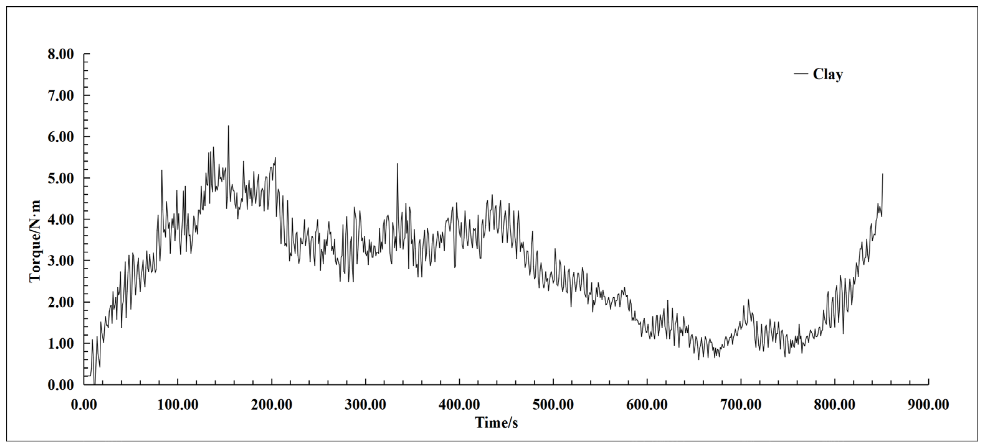
Before starting the stirring test, fix the test bucket with soil samples under the agitator to ensure that the bucket can be shifted or rotated in any way during the whole test. After the bucket is fixed, start the equipment and set the rotation speed of the mixing agitator and the downward speed in the monitoring system. Once the set-up is complete, click “Test Start” in the control system interface. During the penetration process, we need to pay close attention to changes in the soil sample, to avoid the influence of other factors on the test results. At the end of the test, we need to export the torque data. These data are an important basis for evaluating the nature of the soil sample and the effect of penetration, which can also be helpful for numerical validation.

2.3. Test Results

According to the field stratum detection, there are mainly five types of soil layers, i.e., silt, silty soil, clay, fine sand, and pebbles, in the mixing depth range. Deep mixing techniques are mainly used for soft base improvement, and silty soils, as well as clays, are the main soil types in soft foundations. Therefore, we focus on two kinds of soil samples, i.e., silty soil and clay, to carry out in-depth physical modeling tests. Here, we show the results of these two test conditions, as well as the main mechanical parameters of the soil, as displayed in

Table 1. Soils material parameters.

Type	Density, kg/m3	Gravity	Bulk Modulus/Pa	Shear Modulus/Pa	Cohesion/Pa	Angle of Internal Friction/°	Water Content/%
Clay	1840	2.74	5.6 × 106	1.9 × 106	5.20 × 103	6.9	39.8
Silty soil	1560	2.69	1.2 × 106	0.9 × 106	7.6 × 103	1.8	53.8

and Figure 5.

In the physical model tests, a three-blade mixer is used to mix the silty and clay soils, and the rotational speeds of the mixer for the two soil types are, respectively, 10 rpm and 20 rpm; a two-blade mixer is used to mix the clay soil, and the rotational speed of the mixing head is 20 rpm. The descending speed of the mixer for the above three conditions is 0.1 m/min. After completion of the test, the mixer torque histories are plotted according to the torque sensor during the mixing process. Figure 6 and Figure 7, respectively, display the torque histories of the three-blade agitator to mix silt and clay soils. Figure 8 shows the torque history of the two-blade agitator to mix the clay soil. From these figures, the torque of the three-blade agitator is gradually increased to a value of around 23 N·m for the silty soil mixed using a rotational speed of 10 rpm, while the torque curve for the three-blade agitator to mix the clay soil with a rotational speed of 20 rpm oscillates and has peak values smaller than 6 N·m. In comparison, the torque values for the two-blade agitator to mix the clay soil with a rotational speed of 20 rpm are relatively smaller than those for the three-blade agitator. The torque histories (especially in Figure 7 and Figure 8) seem to have obvious oscillations. The oscillations with small amplitudes presented in Figure 7 and Figure 8 are mainly caused by the uneven distribution of soil particles in the soil layer; in addition, there are some relatively large fluctuations in these two figures (e.g., at around 50 s in Figure 8), which have a large effect on the torque. This is due to the fact that during soil preparation, the soil is placed layer by layer into the container of the test set-up, which leads to large fluctuations when the agitator crosses the soil layers.

3. Numerical Simulations

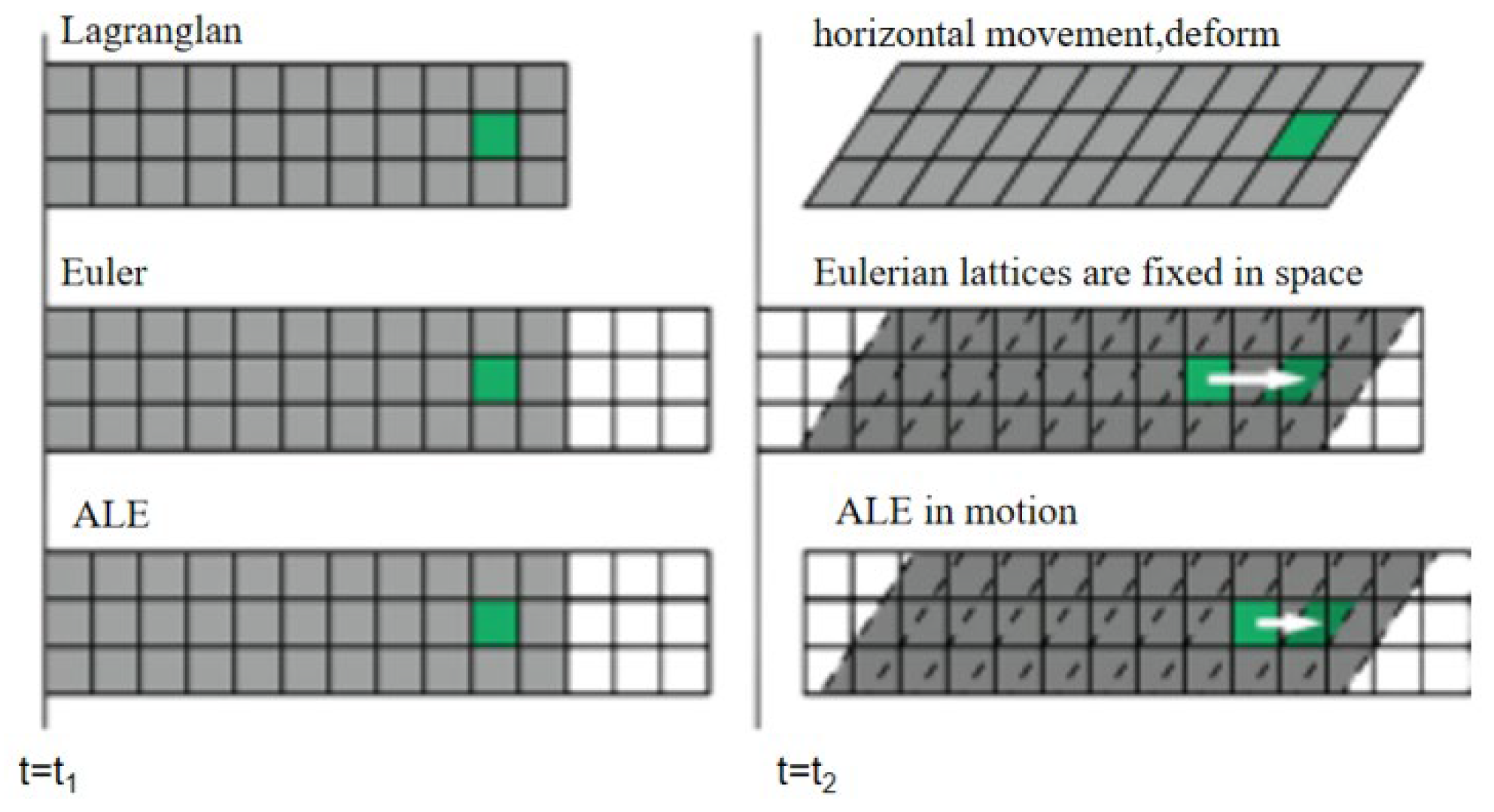
3.1. ALE Method

The fundamental idea of the ALE method is to use the Lagrange method to deal with the boundary motion of the structure, and then to utilize the Euler method to divide the internal mesh, so that the grid cells and material points are independent of each other. The mesh in the ALE method is not exactly the same as that in the Euler method, and the mesh position in the ALE method is adjusted appropriately along with the computational process. In doing so, mesh distortion due to large deformation can be avoided. Figure 9 shows the schematics of grid configurations for Lagrangian, Euler, and ALE algorithms.

The reference domain Ω under the coordinates of the ALE algorithm, the matter domain Ω_L under the coordinates of the Lagrange algorithm, and the spatial domain Ω_E under the coordinates of the Euler algorithm, are defined in the ALE method, respectively. There is a mapping relationship between the three. The matter motion at time t can be described as follows [28].

The mapping from the matter domain Ω_L to the space domain Ω_E is given by:

$$x_E=x\left(X_L,t\right)$$

(1)

The mapping from the reference domain Ω to the spatial domain Ω_E is given by:

$$x_E=\tilde{x}\left(\tilde{x},t\right)$$

(2)

The mapping of the matter domain Ω_L to the reference domain Ω can be derived from Equations (1) and (2) as:

$$\tilde{x}={\tilde{x}}^{-1}\left(x\left(X_L,t\right),t\right)=\psi \left(X_L,t\right)$$

(3)

The equations for conservation of mass, momentum, and energy for the ALE description are expressed separately as follows [29]:

• The equation of conservation of mass can be expressed as:

$$\frac{\partial \rho }{\partial t}=-\rho \frac{\partial \nu }{\partial x_i}-w_i\frac{\partial \rho }{\partial x_i}$$

(4)

where w is the relative velocity with $w=v-u$, and v and u are the motion velocities of the material point in the coordinates of the Lagrange algorithm and the reference point in the coordinates of the ALE algorithm, respectively, which take the forms of:

$$\nu =\frac{\partial \varphi \left(X_L,t\right)}{\partial t}{|}_X$$

(5)

$$u=\frac{\partial \varphi \left(\tilde{x},t\right)}{\partial t}{|}_{\tilde{x}}$$

(6)

The governing equations of the fluid problem are the Navier–Stokes equations under the ALE description.

$$\frac{\partial \nu }{\partial t}=-\left({\sigma }_{ij,j}+\rho b_i\right)-\rho w_i\frac{\partial {\nu }_i}{\partial x_j}$$

(7)

2.

The equation of conservation of mass can be expressed as:

$$\frac{\partial E}{\partial t}=-\left({\sigma }_{ij}{\nu }_{i,j}+\rho b_i{\nu }_i\right)-\rho w_j\frac{\partial E}{\partial x_j}$$

(8)

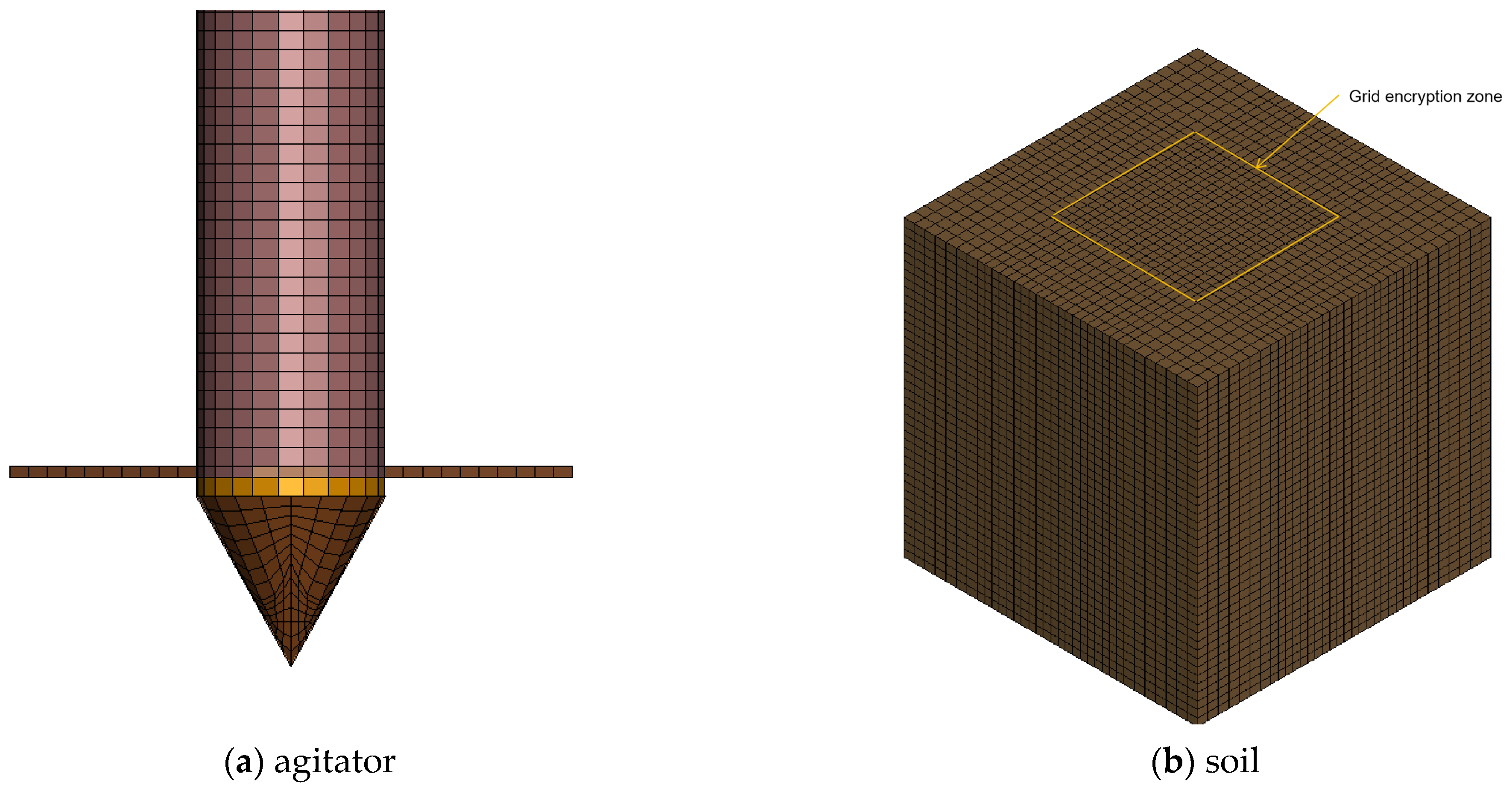
3.2. Numerical Model

To determine the soil grid size, this paper first conducts a mesh convergence test. Three numerical cases that respectively use grid sizes of 8 mm, 10 mm, and 12 mm for the mixing process are accordingly conducted. The soil type considered in these cases is clay soil, and a three-blade agitator is employed with an operation speed of 20 rpm and a downward speed of 0.1 m/min. The torque histories of the agitator during soil mixing of the three cases are compared in Figure 10, where the torques during the stabilization time are taken for comparison. From this figure, one can observe that the differences between the different torque curves are small, and the simulated torque values in the cases with grid sizes of 10 mm and 12 mm are consistent with the corresponding experimental data. In consideration of calculation speed and accuracy, the grid size of the soil for the following numerical cases is set to 10 mm.

To ensure numerical accuracy and stability, the mesh size to discretize the agitator should be similar to that of the soil. That is to say, the average mesh size for the agitator is set to 10 mm, while some small elements with mesh sizes of around 3 mm exist. The schematic of the finite element models for the agitator and the soil is shown in Figure 11. In order to ensure mesh quality, the soil finite element model has a square domain with dimensions of 400 mm × 400 mm × 400 mm, with mesh sizes ranging from 10 mm to 14 mm. The mesh size for the mixing region is 10 mm, and the meshes are coarsened to 14 mm for the boundary. The encrypted area is 200 mm × 200 mm.

As for material models, the mixing agitator is modeled using a linear elastic model with the keyword of MAT_ELASTIC, and the material parameters are detailed in

Table 2. Material parameters for mixing agitator.

Type	Density, kg/m3	Young’s Modulus/Pa	Poisson’s Ratio
Steels	7800	2.1 × 1011	0.3

. The soil characteristics are described using the material model with the keyword of *MAT_FHWA_SOIL [30,31], available in the LS-DYNA code. Note that the code version used in this work is version 970, LSTC, USA. This model accounts for the correction of the Mohr–Coulomb yield criterion, and extends the effects of water content, deformation rate, element deletion, and other functions. It can be regarded as one kind of isotropic material model for solid elements, which considers material loss. The material parameters for the soil are shown in Table 1.

In order to accurately reproduce the test results, boundary conditions need to be carefully set for numerical simulations. The main boundary setting of the mixing head is to limit all its degrees of freedom except for the Z-direction displacement and rotation around the Z-axis, so as to ensure that the mixing head is not deflected due to force deflection during the mixing process. During the model test, the soil is placed in a fixed container with the top surface as the only one free surface. Therefore, fully constrained wall boundaries are applied to the soil in numerical simulations, except for that on the top surface.

The main keywords used for the model construction in LS-DYNA include *DATABASE_CROSS_SECTION_SET, *CONSTRAINED_LAGRANGE_IN_SOLID, *LOAD_BODY_Z, and *BOUNDARY_SPC_SET. Among them, the first keyword defines a cross-section using a point set and a cell set and is used to output cross-section forces; the second one is used to create a contact relationship between the soil and the agitator, where a master–slave configuration is needed, with the agitator as the slave and the soil as the master; the third keyword applies a gravity field to the overall model; the fourth one imposes full constraints on the five surfaces of the soil model, excluding the top surface.

3.3. Numerical Cases and Results

In the present work, with the aid of the aforementioned numerical method and models, we conduct an in-depth study on the mixing behaviors of the agitator blades after they completely enter the soil. In the study, we simulate two different soil types, i.e., clay and silty soils, with a three-blade mixing agitator, and the physical time for numerical cases is set to 10 s. For the clay soil, the speed of the mixing agitator is set to 10 rpm, while for the silty soil, the speed is increased to 20 rpm. In addition, this work also simulates two conditions of clay mixing with a two-blade agitator at 10 rpm and 20 rpm, and the physical time for each case is set to 5 s. The downward speed of the mixing agitator is kept the same in the above cases, i.e., 0.1 m/min. In order to ensure the accuracy of simulation results, we use the same experimental parameters as those in the physical model test. After the simulation is completed, the torque data of the cylindrical cross-section of the mixing agitator during the mixing process are obtained. Figure 12 shows snapshots of the mixing behaviors for the clay soil using a three-bladed mixing agitator, where the soil model is divided into upper and lower parts and set to be transparent for a better presentation of the mixing effect.

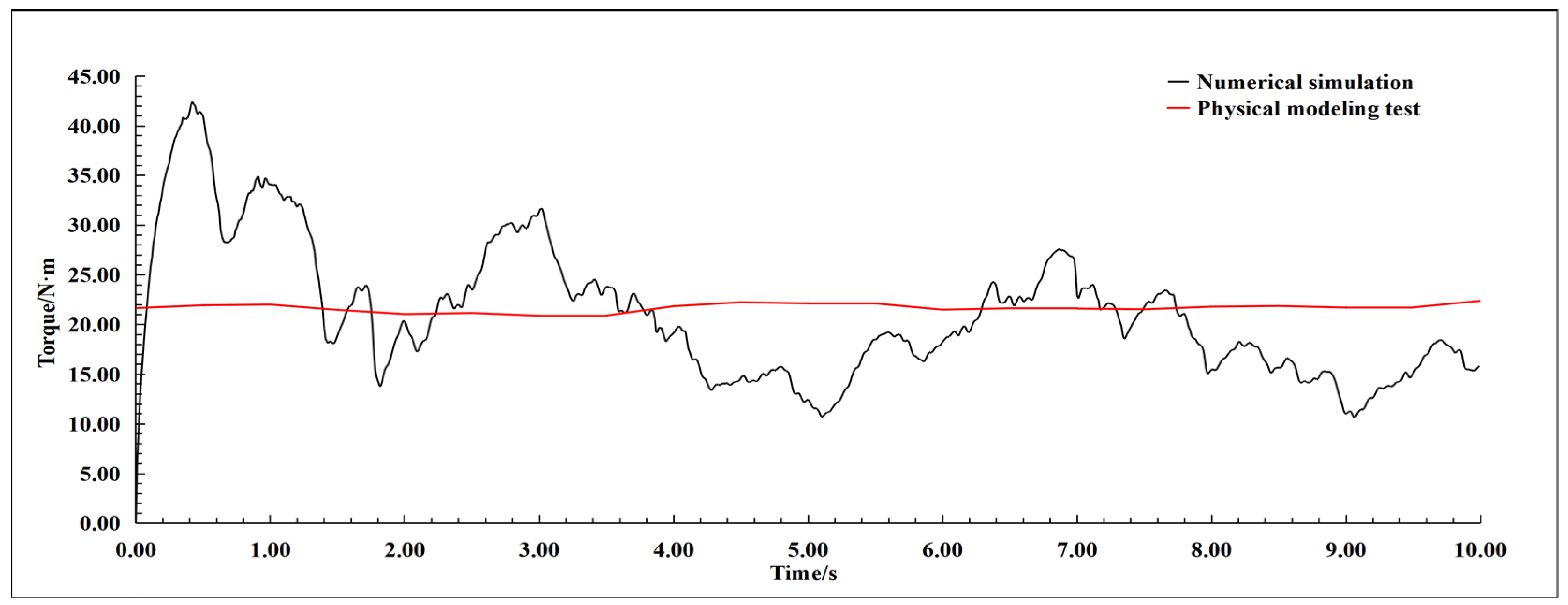
3.3.1. Torque Data for the Three-Blade Mixing Agitator

The simulated torque history to mix the silty soil is compared with the corresponding experimental data in Figure 13, where the experimental torque data are taken from 210 s to 220 s. The average value of torque in the selected time interval is 21.688 N·m, and the numerical simulation value is 21.033 N·m, with an error of 3%. Therefore, the numerical result is in agreement with the experimental data. The adopted explicit time integration scheme for dynamic mixing behaviors contributes to the oscillations of the numerical torque history curve. The comparison of the simulated and experimental torque data for the clay soil is shown in Figure 14, where the experimental torque data are taken from 313 s to 323 s. The average value of torque in the selected time interval is 4.714 N·m, and the numerical simulation value is 5.26 N·m. The error is 11.6%, which is acceptable from the engineering perspective. Therefore, the numerical result is in agreement with the experimental data. The comparisons in the two figures have demonstrated the accuracy and effectiveness of our introduced numerical approach in capturing average torque values of an agitator.

For Figure 13 and Figure 14, as well as Figure 15 in the next subsection, the torque curves start with large values and then gradually decrease, oscillating around the average values. The main reason is that, at the beginning of the mixing process, the agitator is already placed in the soil to save computational cost—soil which is not damaged at that time. This results in large torque values at the beginning. However, as the soil is gradually damaged by the agitator, the torque values required by the agitator gradually decrease and finally oscillate around the mean values.

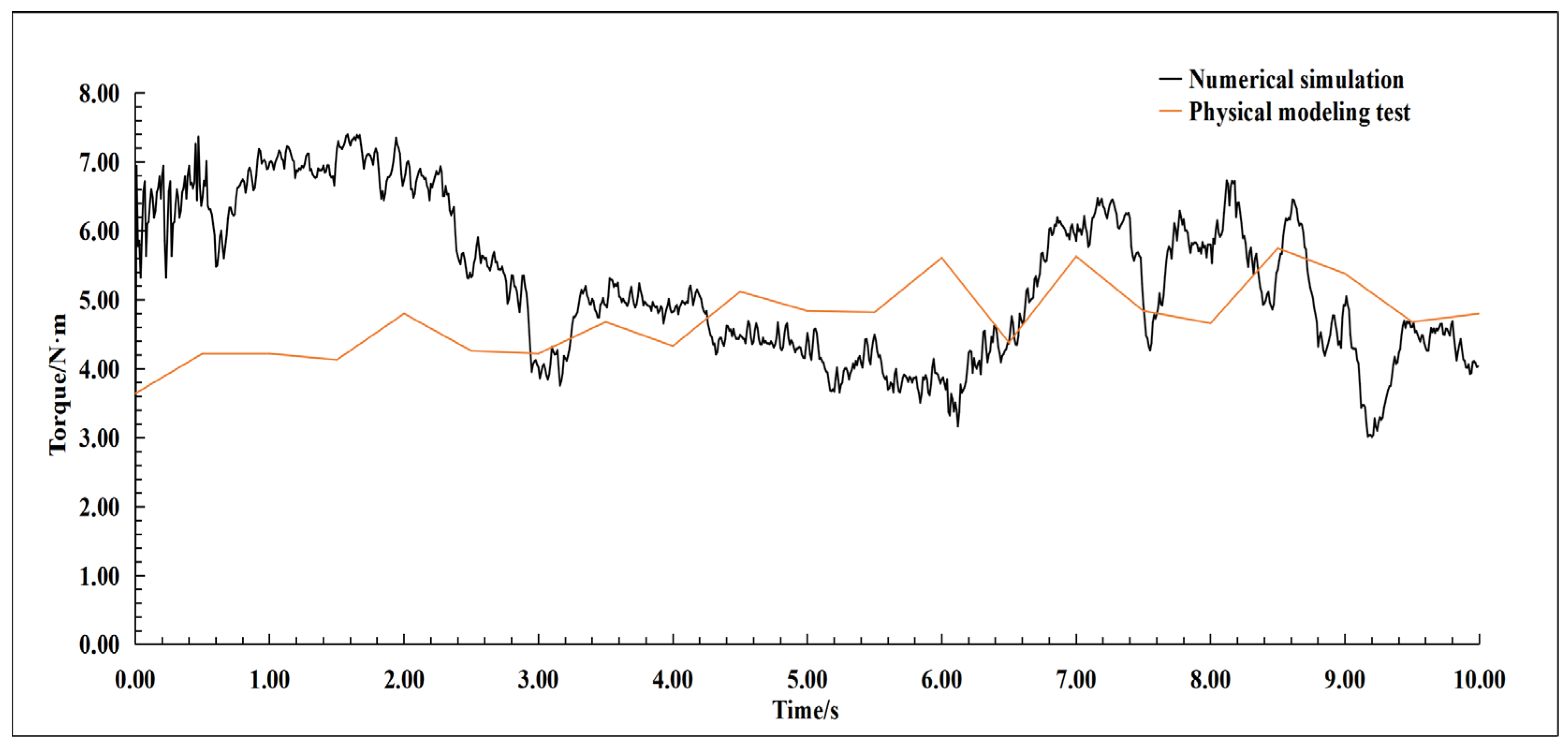
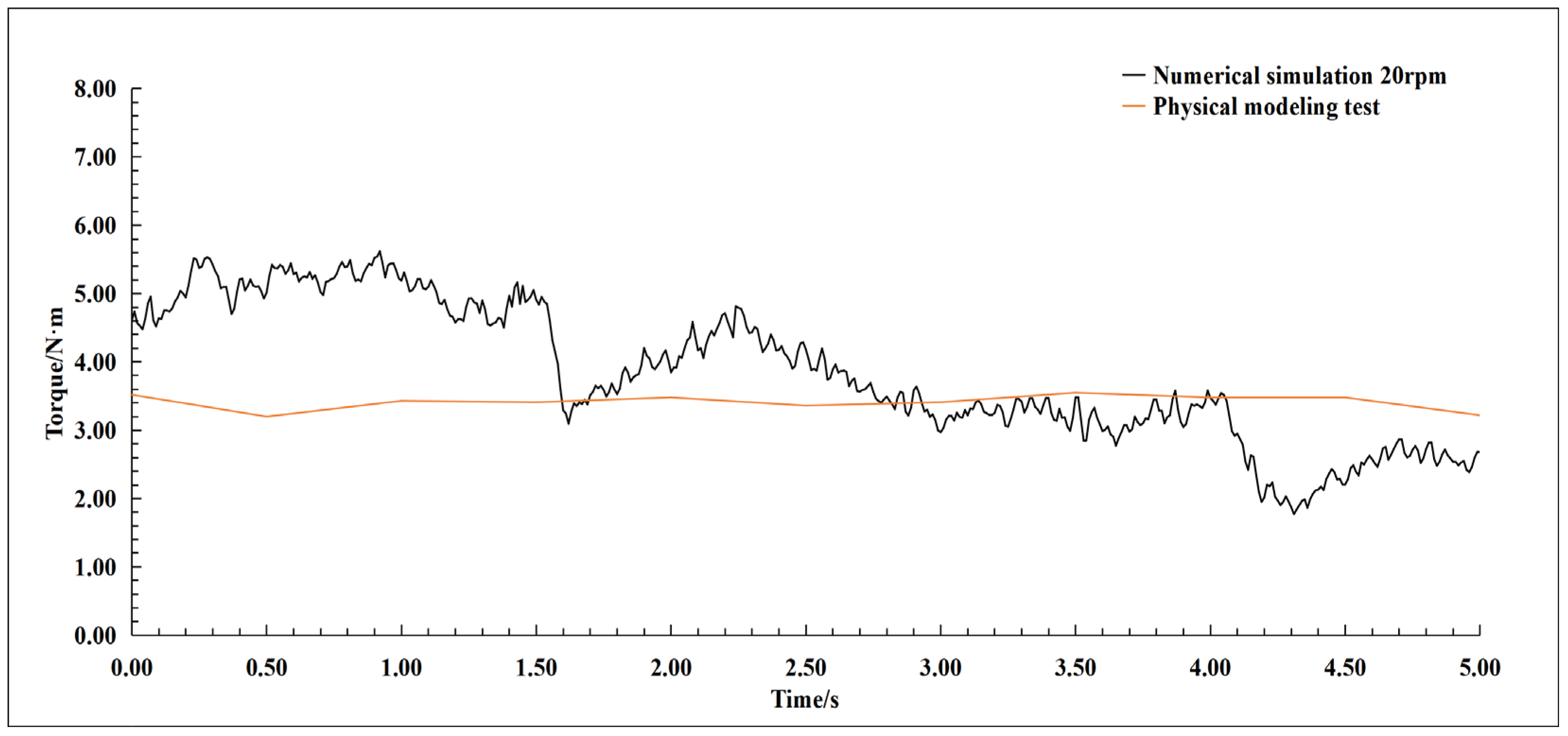
3.3.2. Torque Data for the Two-Blade Mixing Agitator

The torque data obtained from the simulation for the mixing of clay soil using a two-blade mixer at 20 rpm are compared with the corresponding experimental data from the physical model test, as shown in Figure 15. The average value of torque in the selected time interval is 3.412 N·m, and the numerical simulation value is 3.745 N·m. The error is 9.7%, and thus the numerical result is regarded to be in agreement with the experimental data. The experimental torque data are taken from 291 s to 296 s. In addition, a numerical case for the mixing of clay soil with a two-bladed mixer at 10 rpm has been carried out, where the other simulation conditions are the same as those in the case with a rotational speed of 20 rpm. The comparison of torque histories for the two cases with rotational speeds of 10 rpm and 20 rpm is shown in Figure 16. The average values of the two rotational speeds were 3.745 N·m and 4.16 N·m. The difference between the two is 0.415 N·m. One can conclude that the averaged torque value with a larger rotational speed is smaller, while the effects of rotational speed on the torque history are tiny.

3.3.3. Discrepancy Analysis

From the comparisons between experimental and numerical results, one can observe errors between them, which are around or smaller than 10%. The cause of these errors is twofold. Firstly, the soil mesh sizes used in our simulations are larger than the real soil particle sizes. From the perspective of computational mechanics, it is unacceptable to use extremely small mesh sizes in consideration of the computational cost. Secondly, the soil material parameters can be easily changed unpredictably during the test process, resulting in different parameters compared with the initially determined physical ones.

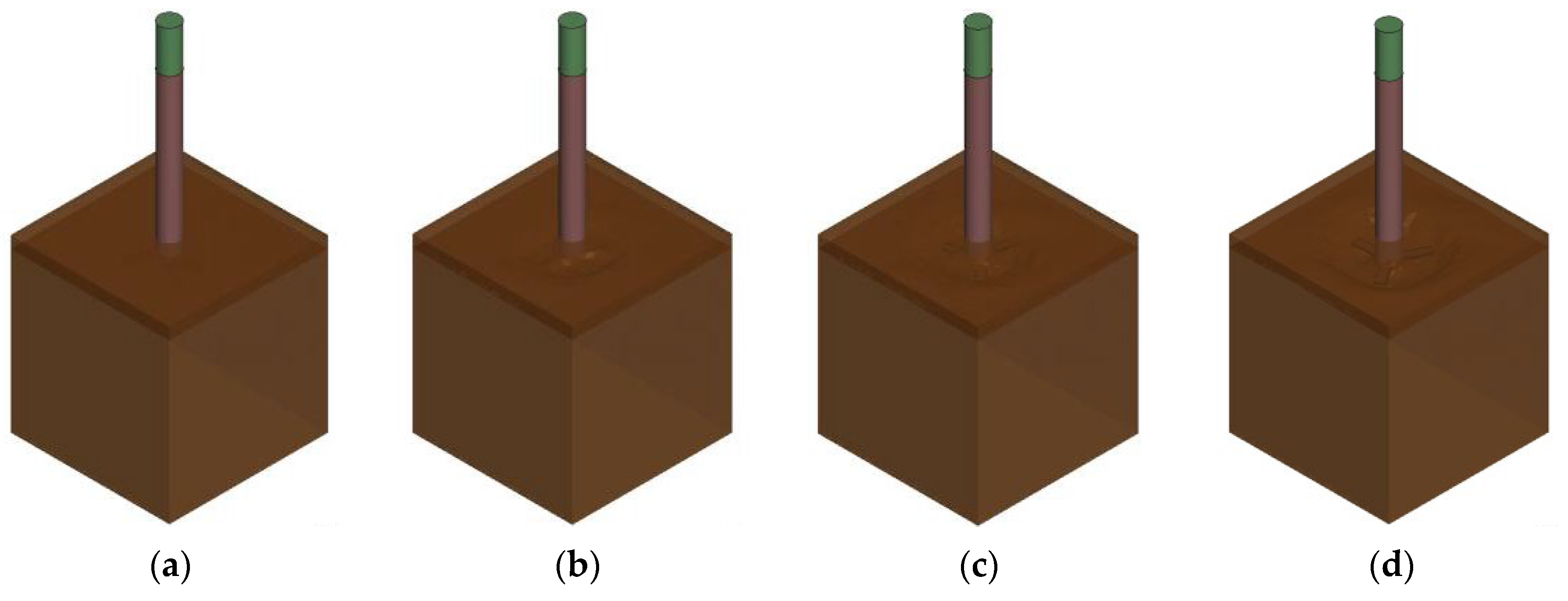
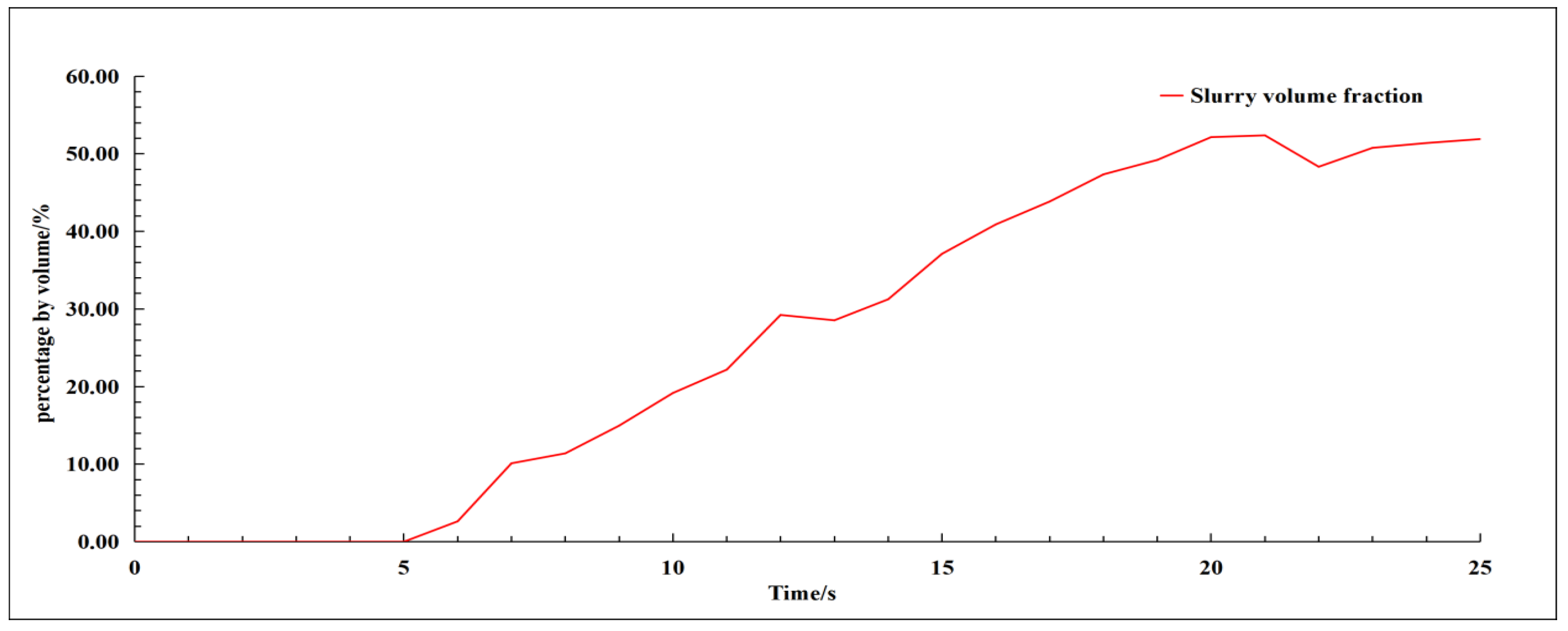
3.3.4. Simulations of Mixing Uniformity

To further demonstrate the capacity of the introduced numerical approach in simulating the homogeneity of the mixing process of cement slurry and soil, this work conducts a numerical case that simplifies the cement slurry injection process. To be specific, the cement slurry is placed on the soil surface, while the mixing agitator is placed in the slurry at the beginning and enters the soil at a downward speed of 1.2 m/min and a rotational speed of 20 rpm. The fluid properties of the cement slurry are described using the Herschel–Bulkley model, corresponding to the material model of MAT_ALE_HERSCHEL [32] in LS-DYNA. The material parameters are listed in

Table 3. Cement slurry material parameters.

Type	Density, kg/m3	Upper Dynamic Viscosity Limit/Pa·s	Lower Dynamic Viscosity Limit/Pa·s	Yield Stress/Pa	Consistency Factor/Pa·Sn
cement paste	0.00183	40	10	0.1	0.449

. The soil type is selected as the clay material mentioned above.

In this work, we describe the homogeneity of mixing in terms of the volume fraction of cement paste in the element, which can be derived from the volume_fraction_mat function in LS-Prepost. We select elements of the mixing region in the center of the soil model for analysis, especially those with depths smaller than the mixer depth at the depth of penetration. This work calculates the volume fraction ratios of materials in the selected region, and it averages the ratios of selected elements to derive the overall volume fraction ratio. The calculated slurry–soil mixing curves are shown in Figure 17. From this figure, one can see that when the mixing agitator has not yet descended to a certain depth (corresponding to 1 s–5 s), as expected, the mud volume percentage in the cell is 0. During the gradual entry of the mixing agitator into the soil (corresponding to 5 s–20 s), the mud percentage is getting higher and higher. This is because the soil and slurry are mixed with each other due to the action of the agitator. Finally, the mud volume percentage tends to be stabilized at about 0.5 (corresponding to 20 s–26 s), which means that the slurry and soil are fully mixed at this moment. The simulated mixing curves are reasonable, which demonstrates the capacity of our introduced method in simulating the mixing behaviors of two different materials.

4. Conclusions

This work has presented experimental and numerical investigations of the mixing behaviors of a scaled DCM mixing agitator. To the best of our knowledge, there are no related publications. The contribution of our work is twofold. Firstly, this work establishes a model test set-up and conducts mixing experiments using two-blade and three-blade mixers. Secondly, we introduce an ALE-based computational method to reproduce the mixing behaviors of DCM agitators. The conclusions of this study are summarized as follows.

(1)

In the model test experiments, when we stir the clay using two- and three-blade agitators, we find that the torque required for the two-blade agitator is slightly larger than that for the three-blade one. The difference between the two is around 1.302 N·m. This difference is not significant, indicating that although the number of blades has an effect on the mixing torque, this effect may not constitute a decisive factor in practice.

(2)

By comparing experimental and simulation results, the capacity of the introduced ALE method in simulating the mixing behaviors of agitators has been demonstrated, but there are some errors. The numerical results show that the average torque value is smaller at a higher rotational speed when the clay is mixed using a two-blade mixer. The difference between the two is 0.415 N·m. The rotational speed has a smaller effect on the torque history.

(3)

In simulating the mixing behavior of two different materials, the homogeneity of the mixing of the two materials can be effectively described using the volume fraction of each material within elements.

In the coming future, our work is scheduled to conduct more experimental and numerical investigations on the mixing behaviors of scaled DCM agitators, by considering more working conditions and the mixing of different materials. The effects of confining stress and complex soil layers [33] (e.g., soil reinforcement layers) on mixing behaviors will be investigated. We will also exploit the capacity of our introduced numerical method in simulating the mixing behaviors of real-scaled DCM agitators, and further validate the accuracy and effectiveness of the numerical method with the aid of in situ experimental data. In addition, it would be useful to establish the relationship between model test results and in situ experimental data. In doing so, one can easily predict the mixing performance of agitators in the in situ construction process on the basis of model test results. In this way, advanced prediction methods based on neural network algorithms [34] will be developed.

References

1. Shu, B.; Gong, H.; Chen, S.; Ren, Y.; Li, Y.; Yang, T.; Zeng, G.; Zhou, M.; Barbieri, D.M.; Li, Y. Case study of solid waste based soft soil solidifying materials applied in deep mixing pile. Buildings 2022, 12, 1193. [Google Scholar] [CrossRef]
2. Su, G.; Liu, H.; Dai, G.; Chen, X.; Deng, Y. Dynamic Analysis of a Concrete-Cored Deep Cement Mixing Pile under Horizontal Dynamic Loads. Buildings 2023, 13, 1378. [Google Scholar] [CrossRef]
3. Bao, H.; Peng, J.; Cheng, Z.; Hong, J.; Gao, Y. Experimental Study on Inner Interface Mechanical Properties of the ESDCM Pile with Steel Core. Buildings 2023, 13, 486. [Google Scholar] [CrossRef]
4. Zhou, M.; Li, Z.; Han, Y.; Ni, P.; Wang, Y. Experimental study on the vertical bearing capacity of stiffened deep cement mixing piles. Int. J. Geomech. 2022, 22, 04022043. [Google Scholar] [CrossRef]
5. Ter-Martirosyan, A.; Sidorov, V.; Sobolev, E. Dynamic Properties of Soil Cements for Numerical Modelling of the Foundation’s Basis Transformed under the Technology of Deep Soil Mixing: A Determination Method. Buildings 2022, 12, 1028. [Google Scholar] [CrossRef]
6. Lee, H.; Kim, S.; Kang, B.; Lee, K. Long-Term Settlement Prediction of Ground Reinforcement Foundation Using a Deep Cement Mixing Method in Reclaimed Land. Buildings 2022, 12, 1279. [Google Scholar] [CrossRef]
7. Wang, N.; Zhang, W. Centrifuge model test of pier ground improved by CDM. Chin. J. Geotech. Eng. 2001, 23, 634–638. [Google Scholar]
8. Hu, Y.; Luo, Q.; Zhang, L.; Huang, J.; Chen, Y. Deformation characteristics analysis of slope soft soil foundation treatment with mixed-in-place pile by centrifugal model tests. Rock Soil Mech. 2010, 31, 2207–2213. [Google Scholar]
9. Zhu, N.; Liu, C.; Wang, W.; Zhao, X. Centrifugal model test on reinforcement methods and consolidation settlement of marshy and lacustrine soft soils. J. Yangtze River Sci. Res. Inst. 2019, 36, 84–89, 97. [Google Scholar]
10. Chi, L.; Kushwaha, R. A non-linear 3-D finite element analysis of soil failure with tillage tools. J. Terramech. 1990, 27, 343–366. [Google Scholar] [CrossRef]
11. Fielke, J. Finite element modelling of the interaction of the cutting edge of tillage implements with soil. J. Agric. Eng. Res. 1999, 74, 91–101. [Google Scholar] [CrossRef]
12. Mouazen, A.; Nemenyi, M. Tillage tool design by the finite element method: Part 1. Finite element modelling of soil plastic behaviour. J. Agric. Eng. Res. 1999, 72, 37–51. [Google Scholar] [CrossRef]
13. Bentaher, H.; Ibrahmi, A.; Hamza, E.; Hbaieb, M.; Kantchev, G.; Maalej, A.; Arnold, W. Finite element simulation of moldboard-soil interaction. Soil Tillage Res. 2013, 134, 11–16. [Google Scholar] [CrossRef]
14. Karmakar, S.; Kushwaha, R. Dynamic modeling of soil-tool interaction: An overview from a fluid flow perspective. J. Terramech. 2006, 43, 411–425. [Google Scholar] [CrossRef]
15. Zhu, L.; Ge, J.; Cheng, X.; Peng, S.; Qi, Y.; Zhang, S.; Zhu, D. Modeling of share/soil interaction of a horizontally reversible plow using computational fluid dynamics. J. Terramech. 2017, 72, 1–8. [Google Scholar] [CrossRef]
16. Shoop, S.; Affleck, R.; Janoo, V.; Haehnel, R.; Barrett, B. Constitutive Model for a Thawing, Frost-Susceptible Sand; U.S. Army Corps of Engineers: Washington, DC, USA, 2005. [Google Scholar]
17. Donéa, J.; Fasoli-Stella, P.; Giuliani, S. Lagrangian and Eulerian finite element techniques for transient fluid-structure interaction problems. In Structural Mechanics in Reactor Technology; CRC Press: Boca Raton, FL, USA, 1977. [Google Scholar]
18. Belytschko, T.; Kennedy, J. Computer models for subassembly simulation. Nucl. Eng. Des. 1978, 49, 17–38. [Google Scholar] [CrossRef]
19. Belytschko, T.; Kennedy, J.M.; Schoeberle, D.F. Quasi-Eulerian finite element formulation for fluid-structure interaction. J. Press. Vessel Technol. 1980, 102, 62–69. [Google Scholar] [CrossRef]
20. Hambleton, J.; Drescher, A. On modeling a rolling wheel in the presence of plastic deformation as a three-or two-dimensional process. Int. J. Mech. Sci. 2009, 51, 846–855. [Google Scholar] [CrossRef]
21. Bekakosa, C.; Papazafeiropoulosb, G.; O’Boya, D.; Prinsc, J.; Mavrosd, G. Dynamic response of rigid wheels on deformable terrains. J. Adv. Veh. Eng. 2016, 2, 210–218. [Google Scholar]
22. Bekakos, C.; Papazafeiropoulos, G.; O’Boy, D.; Prins, J. Finite element modelling of a pneumatic tyre interacting with rigid road and deformable terrain. Int. J. Veh. Perform. 2017, 3, 142–166. [Google Scholar] [CrossRef]
23. Zhang, L.; Cai, Z.; Liu, H. A novel approach for simulation of soil-tool interaction based on an arbitrary Lagrangian–Eulerian description. Soil Tillage Res. 2018, 178, 41–49. [Google Scholar] [CrossRef]
24. Li, J. Study on 3D-Dynamic Simulation of Shield Cutter. Ph.D. Dissertation, Tianjin University, Tianjin, China, 2019. [Google Scholar]
25. Ding, J.; Jin, X.; Guo, Y.; Tang, H.; Yang, H. Study on 3-D Numerical simulation for soil cutting with large deformation. Trans. Chin. Soc. Agric. Mach. 2007, 38, 118–121. [Google Scholar]
26. Shen, J.; Jin, X.; Yang, J.; Ling, Y. Dynamic Numerical Simulation of Excavation in Shield Tunnelling. J. Shanghai Jiaotong Univ. 2009, 43, 1017–1020. [Google Scholar]
27. Shen, J.; Jin, X.; Li, Y.; Wang, J. Numerical simulation of cutterhead and soil interaction in slurry shield tunneling. Eng. Comput. 2009, 226, 985–1005. [Google Scholar] [CrossRef]
28. Soulaimani, A.; Saad, Y. An arbitrary Lagrangian-Eulerian finite element method for solving three-dimensional free surface flows. Comput. Methods Appl. Mech. Eng. 1998, 162, 79–106. [Google Scholar] [CrossRef]
29. Souli, M.; Ouahsine, A.; Lewin, L. ALE formulation for fluid–structure interaction problems. Comput. Methods Appl. Mech. Eng. 2000, 190, 659–675. [Google Scholar] [CrossRef]
30. Lewis, A. Manual for LS-DYNA Soil Material Model 147 (No. FHWA-HRT-04-095); Federal Highway Administration: Washington, DC, USA, 2004. [Google Scholar]
31. Reid, J.; Coon, B.; Lewis, B.; Sutherland, S.; Murray, Y. Evaluation of LS-DYNA Soil Material Model 147 (No. FHWA-HRT-04-094); Federal Highway Administration: Washington, DC, USA, 2004. [Google Scholar]
32. MANUAL, K.U.S. LS-DYNA Keyword User’s Manual; LSTC Co.: Livermore, CA, USA, 2007. [Google Scholar]
33. Huynh, V.H.; Nguyen, T.; Nguyen, D.P.; Nguyen, T.S.; Nguyen, T.C. A novel direct SPT method to accurately estimate ultimate axial bearing capacity of bored PHC nodular piles with 81 case studies in Vietnam. Soils Found. 2022, 62, 101163. [Google Scholar] [CrossRef]
34. Nguyen, T.; Ly, K.D.; Nguyen-Thoi, T.; Nguyen, B.P.; Doan, N.P. Prediction of axial load bearing capacity of PHC nodular pile using Bayesian regularization artificial neural network. Soils Found. 2022, 62, 101203. [Google Scholar] [CrossRef]
Figure 1. A schematic diagram of a DCM ship.
Buildings 14 01809 g001
Figure 2. Geometrical and physical models of our established experimental set-up. An additional operating device is involved in (b) at the right side when compared with the devices in (a).
Buildings 14 01809 g002
Figure 3. Physical models of a three-bladed agitator and a torque transducer. (a) The physical model of a three-bladed stirrer; (b) the physical model of a transducer connector; (c) the physical model of a transducer.
Buildings 14 01809 g003
Figure 4. A schematic of the arrangement form of the power head.
Buildings 14 01809 g004
Figure 5. Mixing behaviors with two different soils.
Buildings 14 01809 g005
Figure 6. The torque history of the three-blade agitator to mix silty soil.
Buildings 14 01809 g006
Figure 7. The torque history of the three-blade agitator to mix clay soil.
Buildings 14 01809 g007
Figure 8. The torque history of the two-blade agitator to mix clay soil.
Buildings 14 01809 g008
Figure 9. Schematics of grid configurations for Lagrangian, Eulerian, and ALE algorithms.
Buildings 14 01809 g009
Figure 10. Comparisons of torque histories in mesh convergence test.
Buildings 14 01809 g010
Figure 11. Finite element meshes for agitator and soil.
Buildings 14 01809 g011
Figure 12. Snapshots of the mixing behaviors for the clay soil using a three-bladed mixing agitator. (a) t = 0 s; (b) t = 2.5 s; (c) t = 5.0 s; (d) t = 7.5 s.
Buildings 14 01809 g012
Figure 13. Comparison of numerical and experimental results for silty soil with three-blade mixing agitator.
Buildings 14 01809 g013
Figure 14. Comparison of numerical and experimental results for clay soil with three-blade mixing agitator.
Buildings 14 01809 g014
Figure 15. Comparison of numerical simulation and experimental results for clay with two-blade mixing agitator.
Buildings 14 01809 g015
Figure 16. Comparison of simulated torque histories with respective rotational speeds of 10 rpm and 20 rpm.
Buildings 14 01809 g016
Figure 17. Simulated slurry–soil mixing curves using our introduced numerical method.
Buildings 14 01809 g017