Interlayer Performance, Viscoelastic Performance, and Road Performance Based on High-Performance Asphalt Composite Structures

Abstract

Weaknesses generated in asphalt pavement structures have a serious impact on the service life of pavements. In order to improve such situations and achieve the goal of enhancing the durability of the pavement structure, this study assesses the performance of heavy-duty asphalt and high-viscosity asphalt, using four high-performance asphalt mixtures: heavy-duty AC-20, high-viscosity AC-20, heavy-duty SMA-13, and heavy-duty SMA-10. Three composite pavement structures were designed: 3 cm SMA-10 + 3 cm SMA-10, 4 cm SMA-13 + 4 cm SMA-10, and 6 cm SMA-13 + 4 cm AC-20. Interlayer performance analysis was conducted on single-layer and composite structures through oblique shear tests; dynamic modulus, fatigue life, and antirutting performance tests on asphalt pavement structural layers were designed and conducted, and the durability performance of high-performance asphalt pavement structural layers was evaluated. The experimental results show that the shear strength of heavy-duty AC is higher than that of heavy-duty SMA, the 4 + 4 combination structure has the best shear strength, the 6 + 4 combination structure has the best structural performance and fatigue resistance, and the 3 + 3 combination structure has the best high-temperature antirutting performance. The comprehensive performance of the 4 + 4 structure is the best among the three combined structures, followed by that of the 6 + 4 structure, and the performance of the 3 + 3 structure is the worst. In addition, this study used bonding energy as an evaluation index and verified the applicability of the bonding energy evaluation index by studying four types of single-layer pavement structures and three types of composite pavement structures.

1. Introduction

With the continuous increase in population and urbanization levels, road construction has been consistently evolving. Under the combined influence of environmental factors and vehicle loads, the predominant distresses generated in roads are rutting and cracks [1,2,3]. The rapid increase in road traffic volume and vehicle axle loads poses new challenges to the design of pavement structures. Consequently, research on the design of high-performance asphalt pavement composite structures has emerged, aiming to enhance pavement load-carrying capacity, durability, and comfort.

Wang et al. [4] investigated the design methods and pavement performance of high-modulus asphalt mixtures and predicted the expected lifespan of bridge pavement structures based on rut deformations. The results demonstrated that using high-modulus asphalt mixtures as the bottom asphalt layer reduced the stress levels in the pavement structure. The novel high-modulus asphalt mixture exhibited excellent comprehensive performance, with a dynamic stability of 9632 cycles/mm and a fatigue life of 1.65 million cycles. Based on rut depth predictions, the adoption of high-modulus mixtures in bridge pavement extended the service life from 5 to 10 years, significantly improving the durability of the pavement structure.

OuYang et al. [5] proposed a new method to resist rutting by increasing the modulus of asphalt concrete, and they studied the impact of high-modulus asphalt concrete on rutting from a mechanical perspective. The results indicate that enhancing the dynamic stability and modulus of HMAC was beneficial for rut prevention. Mechanical calculations revealed that the maximum shear stress occurred in the intermediate layer of the pavement structure. HMAC could increase the elastic modulus of the intermediate layer and improve the stress state of the pavement structure, reducing shear strain and preventing rutting in asphalt pavement. Qian et al. [6] compared the high-temperature performance, low-temperature crack resistance, fatigue resistance, and water stability of rigid asphalt, heavy-duty AH-70, and styrene–butadiene–styrene (SBS) polymer-modified asphalt mixtures. The results showed that rigid asphalt mixtures exhibited significant high-temperature performance. Si et al. [7] conducted indoor tests and DEM simulations of uniaxial compression on HMAC pavement structure materials. They analyzed the displacement and stress distribution in the vertical and horizontal directions, as well as the horizontal shear stress. The results revealed that HMAC pavement had less maximum vertical displacement. The application of HMAC reduced the vertical stress in all structural layers except the surface layer, lowered the horizontal stress in the base layer, and enhanced the deformation resistance of asphalt pavement.

The experimental results of Geng et al. [8] indicate that, compared to traditional asphalt and styrene–butadiene–styrene (SBS)-modified asphalt, high-viscosity asphalt exhibits significantly improved resistance to high-temperature rutting and low-temperature cracking. Subsequently, they designed Stone Matrix Asphalt (SMA) asphalt mixtures containing this high-viscosity asphalt using the Marshall method and studied its engineering performance. The test results demonstrate that incorporating high-viscosity asphalt, compared to SBS-modified asphalt, results in better fatigue performance and water resistance. Qin et al. [9] studied the high-temperature performance of high-viscosity asphalt through temperature scanning and frequency scanning tests, demonstrating a significant improvement in the rutting resistance of high-viscosity asphalt. Rutting tests further revealed the excellent high-temperature characteristics of high-viscosity asphalt mixtures, indicating consistency in high-temperature performance between asphalt and asphalt mixtures. Zhou et al. [10] introduced a certain amount of SBS modifier, viscosity-increasing resin, stabilizer, and plasticizer into base asphalt to prepare a high-viscosity modified asphalt (HVMA) with outstanding performance. Comparative tests were conducted against domestically produced high-viscosity asphalt (HVA). The study showed that HVMA exhibited excellent high-temperature rutting resistance and resistance to permanent deformation, comparable to HVA.

Arnold et al. [11], focusing on rutting distress at road intersections, conducted performance tests on the high-modulus asphalt mixture EME. The results indicate that the rutting resistance of high-modulus asphalt mixtures was 100 times higher than that of other mixtures. Simultaneously, this high-modulus asphalt mixture, with a higher asphalt content, exhibited improved modulus and fatigue properties, allowing for a one-third reduction in pavement thickness. Maria et al. [12] conducted a study on the influence of temperature on high-modulus asphalt mixtures using five hard asphalts. The results demonstrate that high-modulus asphalt mixtures produced with hard asphalts maintained high-modulus values even at high temperatures. This application, suitable for airport pavement base layers, allows for a significant reduction in pavement thickness while enhancing pavement fatigue performance.

Another study indicated excellent rutting resistance for all three mixtures, with rubberized asphalt exhibiting 17.1% to 30.5% higher fracture energy than the control and 6.8% to 9.1% higher than the polymer mix. Both rubber and polymer enhance asphalt’s resistance to permanent deformation and fatigue life. Dry-processed rubberized asphalt demonstrates superior cracking resistance and fatigue life, suitable for high-volume roads in Michigan’s wet-freeze conditions [13]. Cold-in-place recycling (CIR) was an effective method for asphalt pavement rehabilitation. However, high air voids and moisture susceptibility were challenges. This study showed a drop in dynamic modulus and rutting resistance after freeze–thaw, with softer binders improving fatigue and low-temperature resistance but reducing rutting resistance. Pavement design analysis indicated increased rutting, cracking, and roughness. CIR enhances cracking and fatigue resistance, making it suitable for low-traffic roads [14]. Asphalt emulsion and hot rubber chip seals were compared in lab tests. Hot rubber chip seals showed higher interlayer shear/tensile strength (48–111% and 36–102% higher) and better aggregate retention and cohesive strength. Both are suitable for pavement maintenance despite weak bonds under cyclic load and freeze–thaw [15]. Zeng et al. [16] conducted a comparative study on the performance of low-penetration hard asphalts and mixtures from China and France. By evaluating the field performance of high-modulus asphalt mixtures, the feasibility of their application in engineering was confirmed. The results indicated that the performance indicators of Chinese and French asphalts met the requirements of high-modulus asphalt mixtures, although there were slight differences in the performance of the two asphalts and their corresponding mixtures. Mixtures of low-penetration hard asphalt with high-modulus asphalt show promising applications in road engineering in China.

Vaitkus et al. [17] conducted indoor tests on high-modulus asphalt concrete mixtures with different aggregate and binder types. The results showed that high-modulus asphalt concrete has a positive effect on improving the performance of urban street pavement. A case study covering the asphalt pavement on Beijing West Chang’an Street with a high-viscoelastic modified asphalt overlay suggests that high-viscoelastic asphalt exhibits excellent performance. It possesses high fatigue resistance and deformation resistance, effectively reducing reflective cracks and moisture damage in the pavement structure while maintaining good pavement service indicators [18,19].

Building on the high performance of materials, this study further focuses on proposing typical pavement structures. Based on the working environment and stress analysis of the pavement layers, this study determined experimental parameters, including the incline angle for the slant shear test on high-performance asphalt structural layers. Four asphalt mixtures and three composite asphalt pavement layers were tested to determine normal stress and optimal shear strength. Through the slant shear test, practical displacement evaluation criteria for bond energy were established for the four high-performance asphalt mixtures. The reliability of the proposed bond energy standard was then verified within the three high-performance asphalt pavement layers. For typical pavement structures, this study proposes three composite structural paving schemes: 3 cm + 3 cm (SMA-10 on top and SMA-10 below), 4 cm + 4 cm (SMA-13 on top and SMA-10 below), and 6 cm + 4 cm (SMA-13 on top and AC-20 below). Utilizing a universal testing machine (UTM), dynamic modulus tests were conducted, and fatigue life and rutting resistance tests for the high-performance asphalt pavement structural layers were designed and performed to evaluate their durability performance.

2. Materials and Methods

2.1. Materials

The asphalt, utilizing high-viscosity asphalt, heavy-duty asphalt, and the bonding layer employing modified emulsified asphalt, yielded the experimental results as presented in

Table 1. Technical indicators of high-viscosity asphalt performance.

Experimental Indicators	Test Result	Experimental Methods
Needle penetration (25 °C, 100 g, 5 s)/0.1 mm	65.0	T0604-2011
Softening point (global method)/°C	88.3	T0606-2011
Elongation (5 °C, 5 cm/min)/cm	40.0	T0605-2011
Dynamic viscosity (60 °C)/Pa·s	61,768	T0607-2011
Flash point/°C	290	T0615-2011
Elastic recovery (25 °C)/%	91	T0611-2011
Solubility (trichloroethylene)/%	99.3	T0610-2011
Thin film heating (mass change)/%	−0.01	T0604-2011
Film heating (residual needle penetration ratio)/%	92.5	T0606-2011
Thin film heating (residual ductility (5 °C))/cm	35.2	T0605-2011

,

Table 2. Technical indicators of heavy-duty asphalt performance.

Experimental Indicators	Test Result	Experimental Methods
Needle penetration (25 °C, 100 g, 5 s)/0.1 mm	51.0	T0604-2011
Softening point (global method)/°C	96.8	T0606-2011
Elongation (5 °C, 5 cm/min)/cm	37	T0605-2011
Flash point/°C	334	T0607-2011
Elastic recovery (25 °C)/%	98	T0615-2011
Solubility (trichloroethylene)/%	99.9	T0611-2011
Thin film heating (mass change)/%	−0.07	T0610-2011
Film heating (residual needle penetration ratio)/%	72	T0604-2011
Thin film heating (residual ductility (5 °C))/cm	20	T0606-2011

and

Table 3. Technical indicators of modified emulsified asphalt.

Experimental Project		Test Result	Experimental Methods
Asphalt content/%		65.6	AASHTO T 59-16
Remaining amount on 1.18 mm sieve/%		0.01	T 0652-199
25 °C Saybolt viscosity/s		82	SH/T 0779-2005
Residue properties	25 °C needle penetration/0.1 mm	82	T0604-2011
	Breaking speed/s	63	ASTM D244
	Softening point (global method)/°C	73	T0606-2011
	Solubility (trichloroethylene)/%	99	T0611-2011
	10 °C Elastic recovery/%	70	T0611-2011
Storage stability	1 d	0.2	GB/T37055.4-2020
	5 d	1.5	GB/T37055.4-2020

.

The basic performances of the heavy-duty asphalt, high-viscosity asphalt, and emulsified asphalt all meet the specification requirements.

2.2. Methods

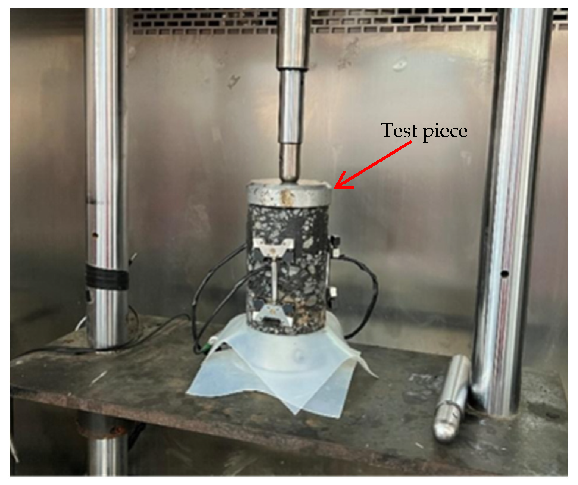
2.2.1. Oblique Shear Test

The inclined shear test is a method commonly used for indoor experimental research in domestic settings. In the experiment, the specimen is placed in a mold and secured with fixtures. A vertical load P is applied, and the specimen is tilted at an angle α. At this point, the vertical load P can be divided into two components, parallel and perpendicular to the bonding interface. In shear tests, the specimen will experience the combined effects of these two forces, causing a distribution of internal shear stress within the specimen. Through the inclined shear test, the shear strength of the specimen can be calculated, and its formulas are given by (1) and (2):

$$\tau =\frac{P\mathrm{s}\mathrm{i}\mathrm{n} \mathsf{\alpha }}{A}$$

(1)

$$\sigma =\frac{P\mathrm{c}\mathrm{o}\mathrm{s} \alpha }{A}$$

(2)

In the formula:

Τ—Shear strength (MPa);

$\sigma$—Normal stress (MPa);

$\mathsf{\alpha }$—The angle between the inclined plane and the horizontal plane;

$P$—Shear force when breaking the ring (N);

A—The stress area of the specimen (m²), for the specimen in the test, A = 0.00785 m².

During the process of vehicle movement, the vehicle load and horizontal shear stress exert forces on the surface of the pavement layer, causing damage or failure in the bonding layer within the pavement structure. To more accurately assess the interlayer bonding strength, multi-angle inclined shear tests can be employed.

In inclined shear tests, altering the shear angle of the specimen allows the force applied to the specimen to closely resemble the actual interlayer stress conditions under different scenarios. Due to time constraints, this study adopts a 30° inclined shear test to evaluate the interlayer bonding strength.

The tests were conducted at a high temperature of 60 °C. Introducing high-temperature conditions can better simulate real environmental conditions and allow studying the performance of asphalt pavement layers under different temperature conditions. The results of these tests can provide a scientific basis for improving the high-temperature resistance of asphalt pavement layers and preventing and managing pavement distress in hot summer weather.

Emulsified asphalt, as a waterproof bonding material in pavement layers, is widely used in pavement construction due to its good adhesion, processability, and durability. In this study, an emulsified asphalt dosage of 0.7 kg/m² was selected.

To investigate the impact of composite pavement structure types, emulsified asphalt dosage, temperature, and other factors on interlayer bonding performance, three pavement types were designed: 3 cm SMA-10 + 3 cm SMA-10; 4 cm SMA-13 + 4 cm SMA-10; and 6 cm SMA-13 + 4 cm AC-20 (referred to as Structure 1, Structure 2, and Structure 3, respectively), with an emulsified asphalt dosage of 0.7 kg/m², a high temperature of 60 °C, and a loading rate of 10 mm/min. Inclined shear tests were used to evaluate the bonding performance of each composite structure, and the specific test plan is outlined in

Table 4. Interlayer bonding test plan.

Composite Pavement Structure Type	Emulsified Asphalt Dosage (kg/m2)	Temperature (°C)
Structure 1	0.7	60
Structure 2	0.7	60
Structure 3	0.7	60

.

Pavement layer shear resistance significantly impacts the durability of the structure. Although various instruments have been used domestically for asphalt pavement interlayer shear tests, a unified testing standard has not yet been established. In this study, shear fixtures suitable for inclined shear tests were developed.

The dimensions and shapes of specimens are typically selected based on the specific testing apparatus used. Common specimen shapes include cylinders and cubes. Although there is currently no unified standard specifying the dimensions and shapes of specimens, the selection should be made based on the specific experimental conditions. Given the varying pavement thickness, structural forms were designed as 3 cm SMA-10 + 3 cm SMA-10; 4 cm SMA-13 + 4 cm SMA-10; and 6 cm SMA-13 + 4 cm AC-20. Therefore, specimen heights included 60 mm, 80 mm, and 100 mm. The specimens were molded into rut shapes using a rutting board and subsequently cut into specimens with a diameter of 100 mm. The types are as shown in

Table 5. Design scheme for shear specimens of pavement layer.

Structural Hierarchy	Test Piece Type
	Type 1	Type 2	Type 3
Superstructure	3 cm SMA-10	4 cm SMA-13	6 cm SMA-13
Type of adhesive layer oil	emulsified asphalt
	3 cm SMA-10	4 cm SMA-10	4 cm AC-20

.

In order to compare the shear strength between composite structures and single-layer structures, specimens of a single type of structure can be molded into rut shapes using a rutting board to form a full-depth shape of 10 cm, resulting in specimens with a diameter of 100 mm.

During the experimental process, a temperature of 60 °C was selected, and the tests were conducted at a shear rate of 10 mm/min until the specimens failed. The specimens were insulated for 2 h prior to the experiment.

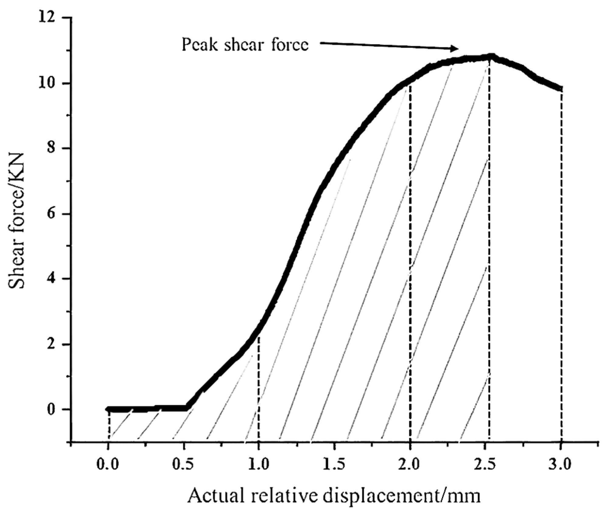
2.2.2. Interlayer Bond Strength Evaluation Based on Energy Method

The interlayer bonding strength of asphalt significantly influences the pavement performance of asphalt, making it crucial to evaluate adhesive strength using appropriate methods [20,21]. This paper employs the energy method to evaluate the interlayer bonding strength. The bonding energy is defined as the integral of shear force with respect to the relative displacement function, where the relative displacement is the sine value of the experimental displacement, as expressed in Equation (3):

$$x=X\mathrm{s}\mathrm{i}\mathrm{n} \alpha$$

(3)

Equation definitions:

$x$—Actual relative displacement (mm);

$X$—Experimental displacement (mm);

$\alpha$—Shear angle.

According to the illustration in Figure 1, the shaded region represents the numerical value of bonding energy. In this study, actual relative displacements of 1 mm, 2 mm, and 3 mm were chosen as calculation standards, and the bonding energy at the shear force peak was computed. Simultaneously, by conducting a correlation analysis between the bonding energy and shear strength for single-type structures, this study aims to propose criteria for calculating bonding energy, facilitating further evaluation of bonding energy between composite structures. In the correlation analysis, the relationship between bonding energy and shear strength is explored through the analysis of experimental data to determine the degree of correlation between bonding energy and shear strength. This allows the establishment of reliable calculation criteria.

2.2.3. Dynamic Modulus Test

When the load frequency applied in indoor experiments is around 10 Hz, it can be considered equivalent to the load applied by a vehicle traveling at speeds of 60–70 km/h on the pavement [22,23]. Dynamic modulus tests can analyze the viscoelastic properties of the composite structures in this chapter. By conducting dynamic modulus tests, the variation in dynamic modulus at different frequencies can be further studied. The experimental setup is illustrated in Figure 2.

Under the specified experimental temperature conditions, the specimen will be subjected to sinusoidal stress at different frequencies during the experiment. By measuring and analyzing the variations in stress and axial strain experienced by the specimen, stress–strain data are obtained. Based on this data, the dynamic modulus and phase angle of the specimen can be calculated. Dynamic modulus refers to the ratio of stress to strain when a material is subjected to periodic loads. The formulas for dynamic modulus and phase angle are given by Equations (4) and (5) [24]:

$$\left|E^{*}\right|=\frac{{\sigma }_0}{{\epsilon }_0}$$

(4)

$$\mathrm{\varnothing }=\frac{T_i}{T_p}\times \left({360}^{\circ }\right)$$

(5)

Equation definitions:

$\left|E^{*}\right|$—Dynamic modulus, MPa

${\sigma }_0$—Amplitude of the sinusoidal load;

${\epsilon }_0$—Amplitude of generated sinusoidal strain;

$\mathrm{\varnothing }$—Phase angle, °;

$T_i$—Time lag, s;

$T_p$—Period of sinusoidal load, s.

Through the use of a gyratory compactor, the bonding layer is formed with emulsified asphalt, creating three composite structures: 3 cm + 3 cm (SMA-10 on top + SMA-10 below), 4 cm + 4 cm (SMA-13 on top + SMA-10 below), and 6 cm + 4 cm (SMA-13 on top + AC-20 below).

Due to the continuous influence of external environmental factors (such as temperature, humidity, traffic loads, etc.) on pavement structures, there is a certain gap between their design standards and reality. This disparity may lead to varying degrees of deviation in the performance of pavement structures, thereby affecting their service life and safety. Therefore, in conducting the asphalt mixture experiments and considering the impact of external environmental factors on pavement structures, the dynamic modulus values of composite structure specimens were tested using a UTM testing machine at temperatures of −10, 4.4, 21.1, 37.8, and 54.4 °C and frequencies of 0.1, 0.5, 1, 5, 10, and 25 Hz to better reflect their actual working conditions.

2.2.4. Analysis of Viscoelastic Properties Based on Haversine Function and CMA Model

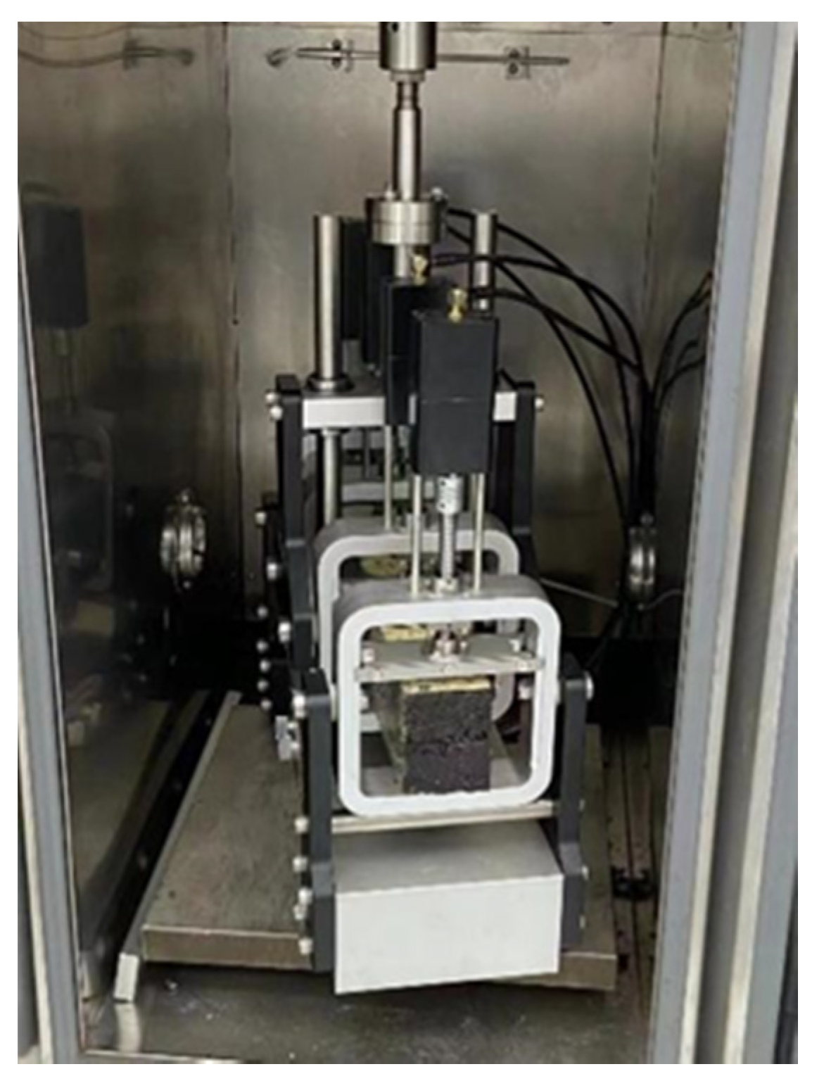
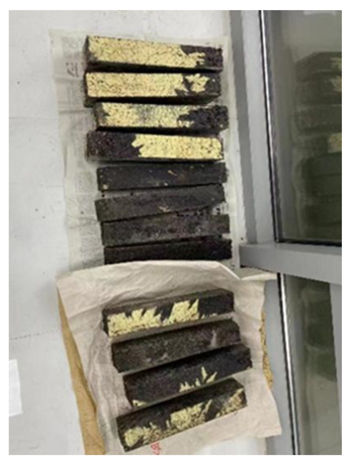
For dynamic modulus test data at different temperatures and frequencies, a portion of the data can be shifted according to the reference temperature or frequency provided by the model. These data are then presented in the form of charts or curves, resulting in a comprehensive dynamic modulus master curve that reflects the mechanical response characteristics of asphalt mixtures under different conditions [25,26].

The shift factor α(T) is defined as the value that moves the frequency level relative to the reference temperature. As shown in Formulas (6) and (7), the logarithm of the reduced frequency is equal to the logarithm of the frequency at the reference temperature plus the logarithm of the shift factor. It is important to note that during the charting process, the reference temperature (T_R) must be explicitly specified. As mentioned earlier, except for the frequency at the reference temperature, which does not need to be shifted, the frequencies at other temperatures need to be shifted. Here, the shift factor at the reference temperature is given as 1, and the most commonly used W.L.F equation is used in this paper. The shift factor α(T) at different temperatures is determined by obtaining the complex modulus and phase angle corresponding to different frequencies at different temperatures. To further process the charts, a nonlinear fitting method is employed to process the data using the sigmoid haversine function as the model, yielding the master curves for complex modulus and phase angle.

$$\mathrm{l}\mathrm{o}\mathrm{g} f_r=\mathrm{l}\mathrm{o}\mathrm{g} f+\mathrm{l}\mathrm{o}\mathrm{g} a\left(T\right)$$

(6)

$$\mathrm{l}\mathrm{o}\mathrm{g} E^{*}=f_r+\frac{\alpha }{1+e^{\beta +\gamma \mathrm{l}\mathrm{o}\mathrm{g} \left(f_r\right)}}$$

(7)

Equation definitions:

$f_r$—Reduced frequency, Hz;

$E^{*}$—Minimum modulus, MPa;

$\mathsf{\beta },\mathsf{\gamma }$—Shape parameters;

$\alpha$—Amplitude of dynamic modulus

Zeng and Bahia, among others [27], proposed the CAM model, which provides a comprehensive expression for the rheological properties of asphalt mixtures and can adapt to different loading conditions.

The CAM model consists of four equations, including the complex modulus master curve equation, storage modulus master curve equation, phase angle equation, and temperature-shift factor equation. These equations are used to depict the viscoelastic proportional relationship and temperature sensitivity of asphalt mixtures.

The equation for the complex modulus master curve in the CAM model is given by Equation (8):

$$G^{*}=G_e^{*}+\frac{G_g^{*}-G_e^{*}}{{[1+{(f_c/f^{\prime })}^k]}^{m_e/k}}$$

(8)

Equation definitions:

$G_e^{*}$—Equilibrium complex modulus, i.e., $G^{*}$(f→0 or at high temperatures);

$G_g^{*}$—Glassy complex modulus, i.e., $G^{*}$(f→∞) or at low temperatures;

$f_c$—Elastic limit threshold;

$f^{\prime }$—Reduced frequency, a function of temperature and strain;

$f_c^{\prime }$—Viscous limit threshold, the frequency at which the asphalt mixture transitions from the viscous flow region to the rheological region;

$m_e$, $k$—Shape parameters or rheological parameters, dimensionless.

The intercepts of G*(f_c) and G_g* on the vertical axis are denoted as R, representing the width of the relaxation spectrum. The specific meaning of R is that the smaller the R value, the more challenging the transition from elasticity to viscosity. The calculation formula for R is given by Equation (9).

$$R=\mathrm{l}\mathrm{o}\mathrm{g} \frac{2^{m_e/k}}{1+(2^{m_e/k}-1)G_e^{*}/{G_g}^{*}}$$

(9)

where the intercepts of G*(fc) and Gg* are on the logarithmic coordinates, also known as rheological parameters.

Asphalt mixtures are viscoelastic materials, and their strength depends on the loading rate (time effect) and test temperature (temperature effect), following the time–temperature superposition principle. Under conditions of uniaxial compression, uniaxial tension, and uniaxial high-strain compression, the time–temperature equivalence principle is effective in understanding the failure and deformation stages of asphalt mixtures [28,29].

Based on the time–temperature equivalence principle, after obtaining the data from the haversine function, the CAM model can be used for fitting to obtain more accurate viscoelastic parameters. The haversine function method is employed to determine high-temperature viscoelastic parameters, which serve as the basis for the nonlinear fitting of the CAM model.

2.2.5. Fatigue Test

To investigate the fatigue performance of asphalt mixtures, many studies employ indoor fatigue testing methods, with the four-point bending fatigue test being widely used [30,31]. In this study, three parallel specimens were prepared for each combination structural scheme. According to the “Test Methods of Asphalt and Asphalt Mixtures for Highway Engineering” (JTG E20-2011), specimens were molded using a rutting board and eventually cut into dimensions of 380 mm × 65 mm × 60 mm (80 mm and 100 mm), as shown in Figure 3 and Figure 4.

Fatigue test parameters:

(1) Flexural tensile strength $\delta t$:

$${\delta }_t=\frac{LP}{w{h}^2}$$

(10)

where:

${\delta }_t$—Flexural tensile strength at the specimen failure (MPa);

L—Span of the bending beam (mm);

P—Maximum load (N);

W—Width of the small beam (mm);

H—Height of the small beam (mm).

(2) Bending strain:

$${\epsilon }_t=\frac{12\delta h}{3L^2-4a^2}$$

(11)

where:

${\epsilon }_t$—Bending strain;

$\delta$—Maximum strain at the center of the small beam;

a—L/3.

(3) Bending stiffness modulus:

$$S=\frac{{\delta }_t}{{\epsilon }_t}$$

(12)

where:

S—Bending stiffness.

2.2.6. Rutting Test

(1)

According to the method outlined in the “Test Procedures for Asphalt and Asphalt Mixtures in Highway Engineering” (JTG E20-2011) [32], rutting test specimens were fabricated using the T0719-2011 procedure, resulting in specimens with final dimensions of 300 mm × 300 mm × 60 mm (80 mm and 100 mm).

(2)

After fabrication, the rutting test specimens were placed within the molds under ambient temperature conditions for no less than 48 h.

(3)

Upon reaching the specified curing time, the specimens along with the molds were placed into the rutting test apparatus, insulated for 5 h, and then subjected to the high-temperature rutting test.

(4)

The rutting test was terminated when the test duration reached 1 h or the maximum deformation reached 25 mm.

3. Results and Discussions

3.1. High-Performance Asphalt Mixture Interlayer Performance Analysis

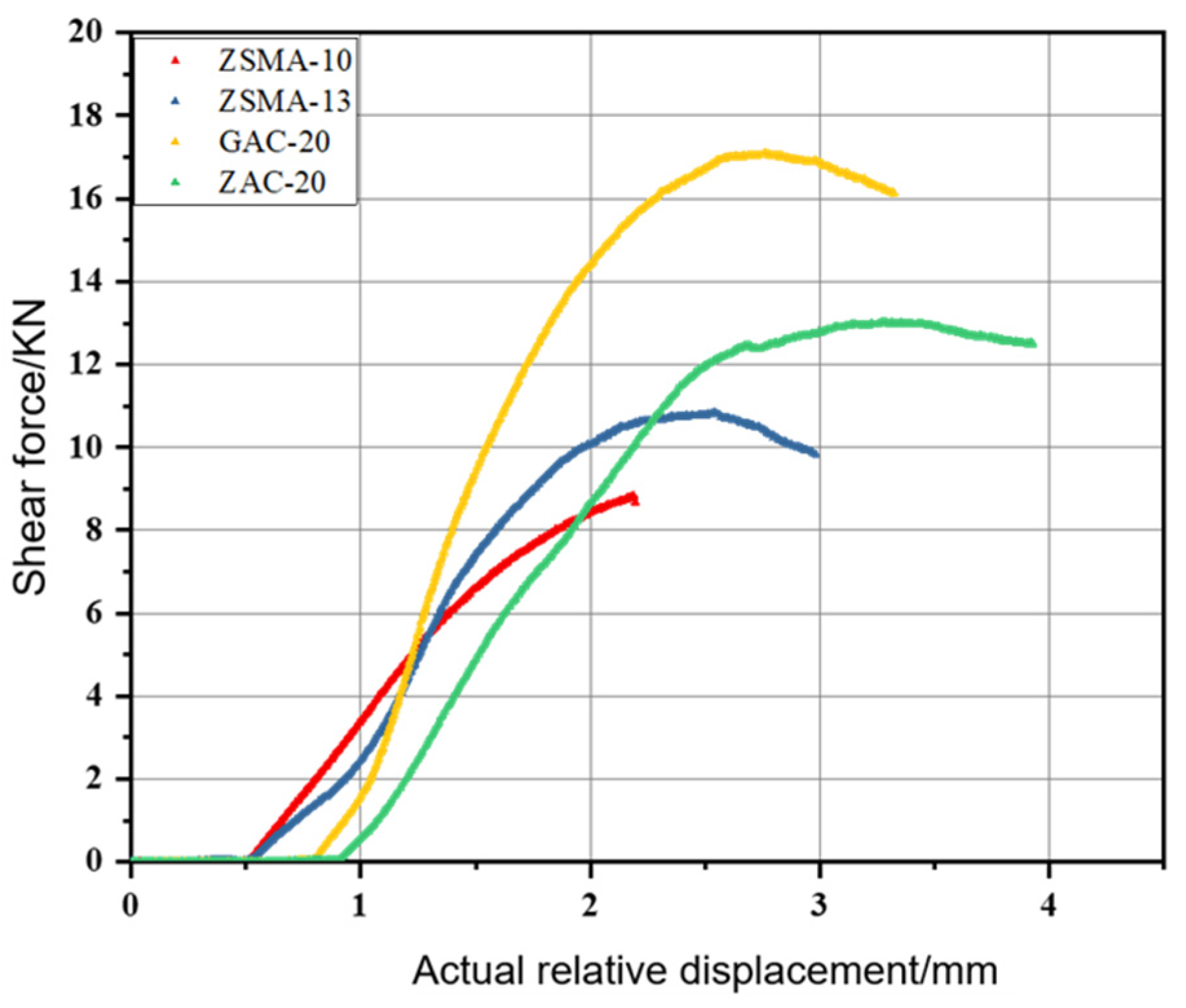
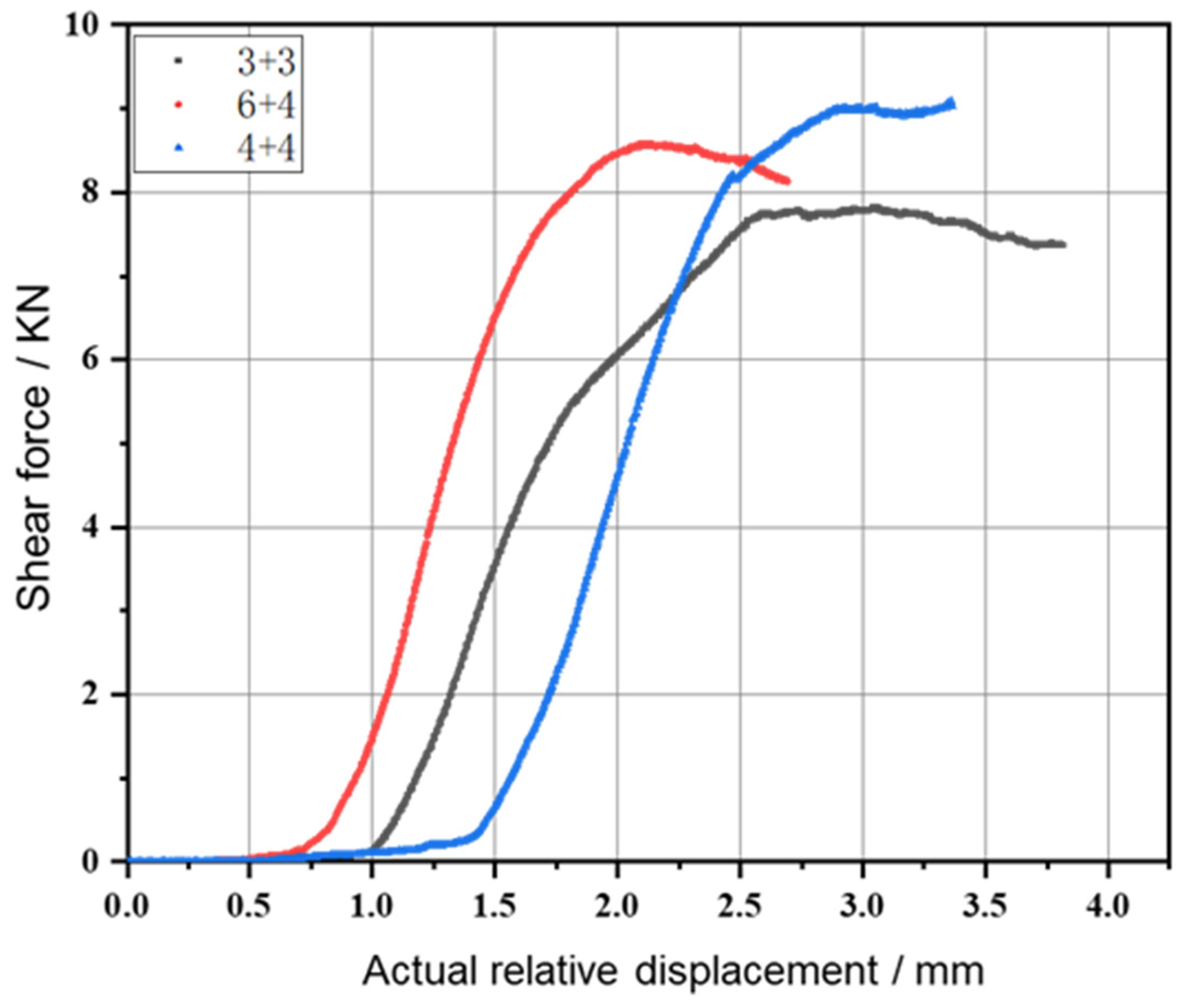
3.1.1. Surface Structure Shear Test Results

Once the specimens meet the high-temperature test conditions, and the temperature in the constant temperature chamber satisfies the requirement of a high-temperature test at 60 °C, shear tests on the specimens can be initiated. The results of the interlayer shear tests for various structures under different test conditions are presented in

Table 6. Results of interlayer adhesion test.

Paving Structure	Emulsified Asphalt Dosage (kg/m2)	Normal Stress (MPa)	Shear Strength (MPa)
Structure 1	0.7	0.86	0.47
Structure 2		0.99	0.57
Structure 3		0.95	0.54
ZAC		1.43	0.83
GAC		1.89	1.08
SMA-10		0.97	0.56
SMA-13		1.20	0.69

.

The interlayer shear strength of pavement composite structures and single-layer structures under different test conditions is shown in Figure 5.

From Figure 5 and Table 6, it can be observed that:

(1) In composite structures, the overall shear strength of Structure 2 and Structure 3 is higher than that of Structure 1. Specifically, the shear strength of Structure 2 is 21% higher than Structure 1, while the shear strength of Structure 3 is slightly higher (0.05 MPa) than Structure 2, representing a small increase. Meanwhile, the shear strength of Structure 3 is 15% higher than Structure 1.

(2) Among single-layer structures, GAC-20 exhibits the highest shear strength, reaching a maximum value of 1.08 MPa. When compared to AC-20 of the same gradation type, the shear strength of the heavy-duty asphalt mixture increases from 0.83 MPa to 1.08 MPa, representing a 30% increase. For the heavy-duty SMA gradation type, the shear strength of SMA-13 is 0.10 MPa higher than SMA-10, indicating a 17% increase.

(3) Further analysis reveals that when asphalt mixtures, i.e., continuous materials, form a composite structure through bonding, the continuity between asphalt layers is disrupted due to the presence of the bonding layer. This leads to the phenomenon where the overall interlayer shear strength of the composite structure is lower than the interlayer shear strength of a single asphalt mixture. Additionally, the higher shear strength of Structures 2 and 3 compared to Structure 1 can be attributed to the selection of asphalt mixtures with higher shear strength, namely ZAC-20 and ZSMA-13.

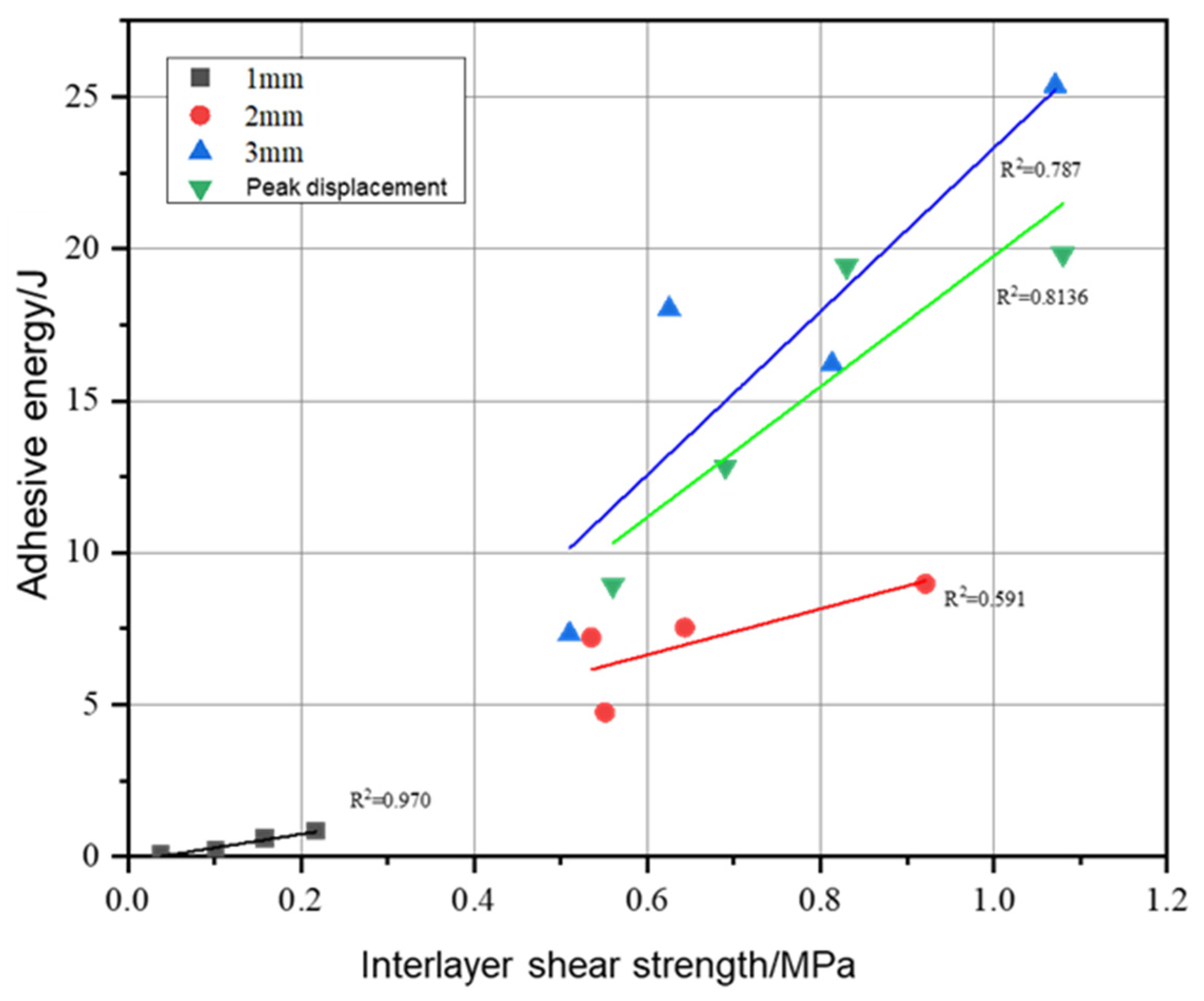
3.1.2. Evaluation and Analysis of Bonding Energy

(1) Single-layer Structure Bonding Energy Evaluation

The shear force–actual relative displacement curves of the four single-layer asphalt mixtures at a 30° shear angle under 60 °C temperature conditions are plotted below. It should be noted that the curves in the initial part of Figure 6 all have a “slip” segment. At this point, due to the small shear force, no relative displacement occurs, resulting in this phenomenon in the graph.

The bonding energy under different calculation standards for the four asphalt mixtures at 60 °C temperature conditions was calculated, and the results are shown in

Table 7. Adhesion energy of four asphalt mixtures.

	Asphalt Mixture	ZSMA-10	ZSMA-13	GAC-20	ZAC-20
Calculation Standard (mm)
1		0.829	0.589	0.217	0.062
2		7.213	7.546	8.979	4.750
3		7.321	18.019	25.378	16.212
Peak displacement		8.933	12.843	19.836	19.430

.

Based on the results in Table 7, the shear strength corresponding to the displacement was found, as shown in

Table 8. Shear strength of four asphalt mixtures.

	Asphalt Mixture	ZSMA-10	ZSMA-13	GAC-20	ZAC-20
Calculation Standard (mm)
1		0.217	0.158	0.102	0.038
2		0.535	0.643	0.921	0.551
3		0.510	0.625	1.071	0.813
Maximum strength		0.56	0.69	1.08	0.83

.

According to the results in Table 7 and Table 8, a correlation analysis of shear strength–bonding energy was calculated and is shown in Figure 7.

At a 60 °C temperature, according to the shear strength–bonding energy relationship curve in the above figure, it can be observed that when the displacement is at 1 mm, although the correlation coefficient reaches 0.970 and shows good data performance, the actual shear strength values corresponding to the 1 mm relative displacement for the four asphalt mixtures are relatively low. This leads to the phenomenon of good correlation at very small displacements and shear strength. In addition, comparing the correlation coefficients of the other three calculation standards: the correlation coefficient of peak displacement is 0.8136 > the correlation coefficient of actual relative displacement at 3 mm (0.787) > the correlation coefficient of actual relative displacement at 2 mm (0.591).

Therefore, through the analysis above, in comparing the bonding energy–shear strength of the four asphalt mixtures, using the peak relative displacement as the indicator associated with shear strength is the most appropriate.

(2) Composite Structure Bonding Energy Evaluation

As shown in Figure 8, it can be observed that among the three composite structures at 60 °C, Structures 6 + 4, 3 + 3, and 4 + 4 reach the shear force peak later, indicating that when Structure 6 + 4 first reaches the peak, it also reaches the maximum limit of the bonding layer’s resistance to shear failure, and its bonding energy also reaches its own limit. The shear force–relative displacement curves of Structures 4 + 4 and 3 + 3 are still difficult to distinguish through graphical analysis, so further analysis is combined with

Table 9. Adhesion energy of three structures.

	Structure Type	3 + 3	6 + 4	4 + 4
Calculation Standard (mm)
2		3.276	6.113	1.385
3		10.609	14.387	9.092
Peak displacement		9.812	11.621	13.619

.

The bonding energy under different calculation standards for the three structures at 60 °C temperature conditions was calculated, and the results are shown in Table 9.

Combining the analysis of graphs and tables, it is observed that the 4 + 4 structure has the highest bonding energy, surpassing the bonding energy of the 3 + 3 structure by 39% and the bonding energy of the 6 + 4 structure by 17%. The bonding energy of the 4 + 4 structure corresponds to the highest shear strength, consistent with the conclusion mentioned in the previous section.

Based on the results in Table 9, the shear strength corresponding to the displacement was found, as shown in

Table 10. Shear strength of three structures.

	Structure Type	3 + 3	6 + 4	4 + 4
Calculation Standard (mm)
2		0.385	0.539	0.296
3		0.465	0.334	0.569
Peak displacement		0.47	0.54	0.57

.

To further validate the applicability of the peak displacement indicator, we obtained the shear strength–bonding energy relationship curves for the three composite structures, as depicted in Figure 9. After eliminating the interference caused by a 1 mm relative displacement, it can be observed that the correlation coefficient for a 2 mm relative displacement is 0.998, for a 3 mm relative displacement is 0.969, and for the peak displacement is 0.967. Among the three evaluation criteria for composite structures, all the obtained correlation coefficients are greater than 0.9, indicating a strong correlation between interlayer shear strength and bonding energy. Although the correlation coefficients for 2 mm and 3 mm relative displacements are both higher than that for peak displacement, in the evaluation criteria for single asphalt mixtures, the correlation with peak displacement is superior. Therefore, considering the bonding energy corresponding to peak displacement in the bonding–shear strength system has significant generalization value.

3.2. High-Performance Composite Structure Viscoelastic Performance Analysis

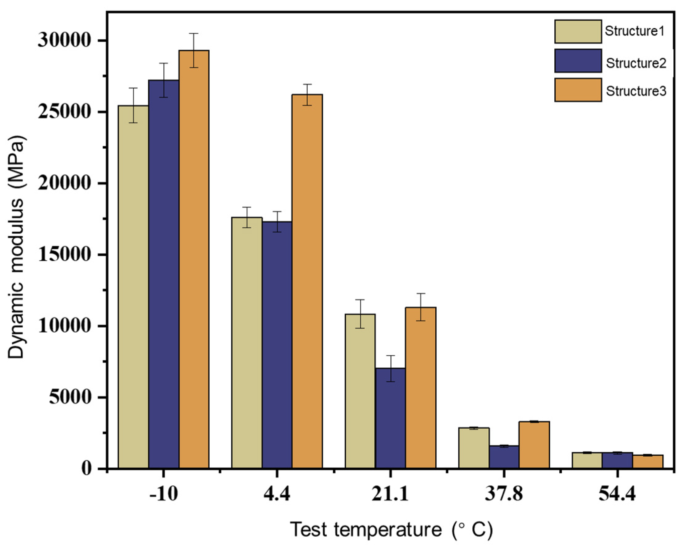
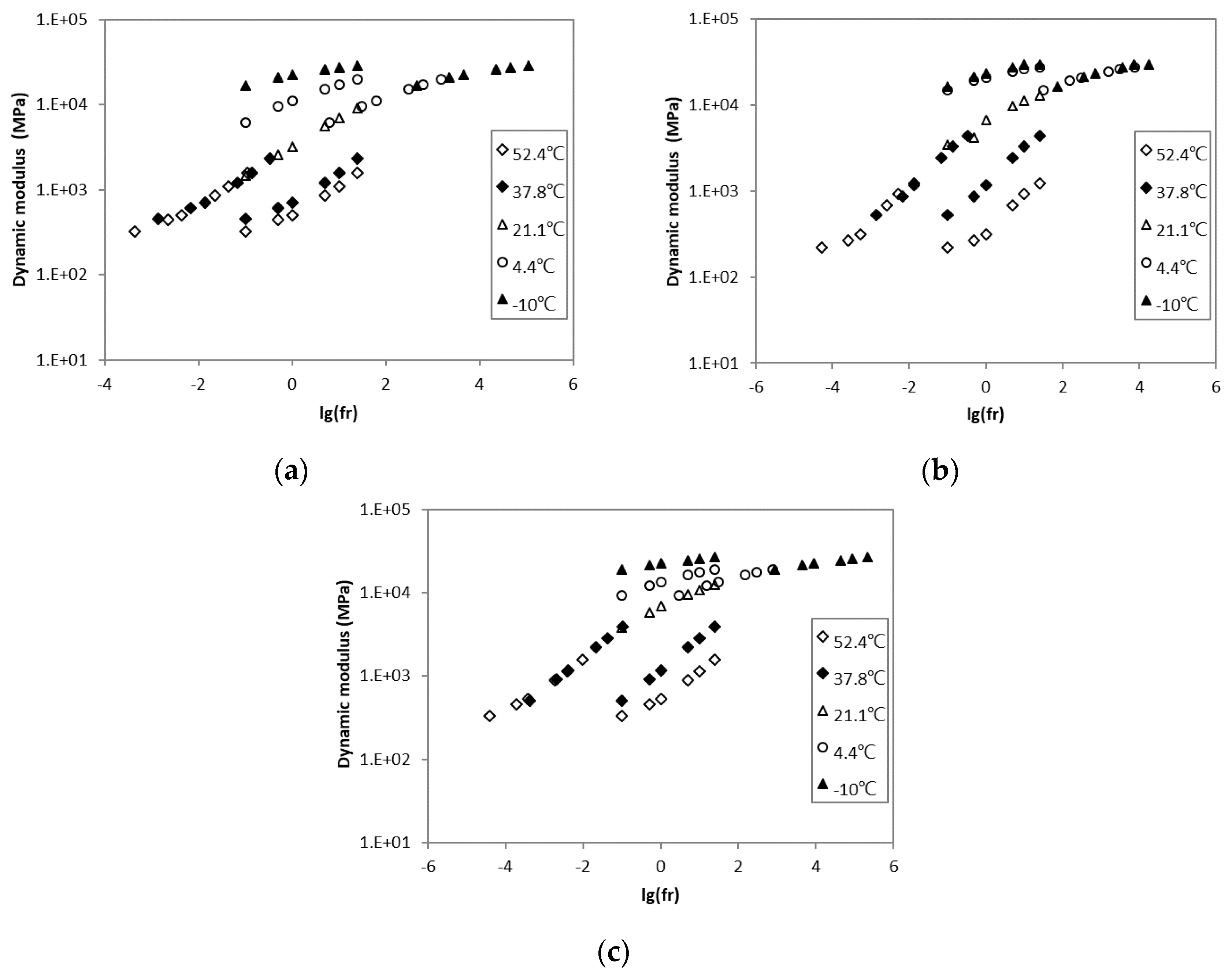
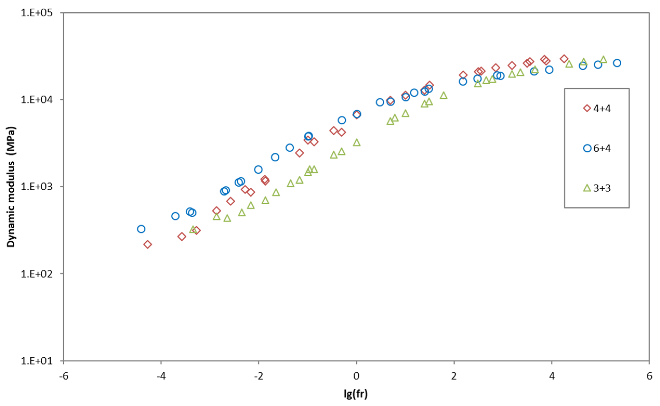
3.2.1. Composite Structure Dynamic Modulus Test Results

The dynamic modulus test results are shown in

Table 11. Dynamic modulus test results for 3 + 3 composite structure asphalt mixes.

Temperature (°C)	Dynamic Modulus at Different Frequencies (Hz)/MPa
	0.1	0.5	1	5	10	25
−10	16,760	20,667	22,281	25,806	27,214	28,877
4.4	6234	9581	11,194	15,325	17,292	19,903
21.1	1474	2539	3220	5666	7017	9052
37.8	459.2	612	702	1202	1580	2344
54.4	323.5	439.8	505	862.9	1104	1593

,

Table 12. Dynamic modulus test results for 4 + 4 composite structure asphalt mixes.

Temperature (°C)	Dynamic Modulus at Different Frequencies (Hz)/MPa
	0.1	0.5	1	5	10	25
−10	16,371	21,380	23,270	27,201	29,292	29,526
4.4	14,794	19,131	20,925	24,644	26,186	27,625
21.1	3454	4218	6703	9823	11,302	12,952
37.8	526.9	870.1	1163	2445	3289	4414
54.4	218.7	26.2	317.7	685.7	936.3	1218

and

Table 13. Dynamic modulus test results for 6 + 4 composite structure asphalt mixture.

Temperature (°C)	Dynamic Modulus at Different Frequencies (Hz)/MPa
	0.1	0.5	1	5	10	25
−10	19,035	21,449	22,412	24,597	25,433	26,698
4.4	9401	12,122	13,352	16,323	17,596	19,211
21.1	3836	5850	6850	9549	10,836	12,566
37.8	503.8	312.1	1168	2217	2841	3888
54.4	329.8	462.2	525.4	890	1128	1580

.

Under the condition of a fixed loading frequency of 10 Hz, the dynamic modulus performance of the three pavement structures at temperatures of −10, 4.4, 21.1, 37.8, and 54.4 °C was investigated. The dynamic modulus test results for the three pavement structures at different temperatures are shown in Figure 10.

According to Figure 10, with the increase in test temperature, the dynamic modulus of the composite structures gradually decreases. This change trend can be explained by the fact that asphalt mixtures are temperature-sensitive viscoelastic materials, exhibiting high-modulus and elastic behavior at low temperatures, and low-modulus and viscoelastic behavior at high temperatures.

When the test temperature is 54.4 °C, the modulus for the 3 + 3 composite structure is 1104 MPa, for the 4 + 4 composite structure is 936.3 MPa, and for the 4 + 6 composite structure is 1128 MPa. The modulus of the composite structure is one of the important indicators of dynamic mechanical response. Therefore, a higher modulus of the composite structure indicates relatively smaller strains generated under external forces, indicating stronger resistance to deformation and better high-temperature stability. Thus, although the high-temperature dynamic modulus of the 6 + 4 structure is close to, but slightly higher than, the other two structures, the 6 + 4 structure (SMA-13 on top + AC-20 on the bottom, Structure 3) is initially selected, indicating its superior high-temperature performance.

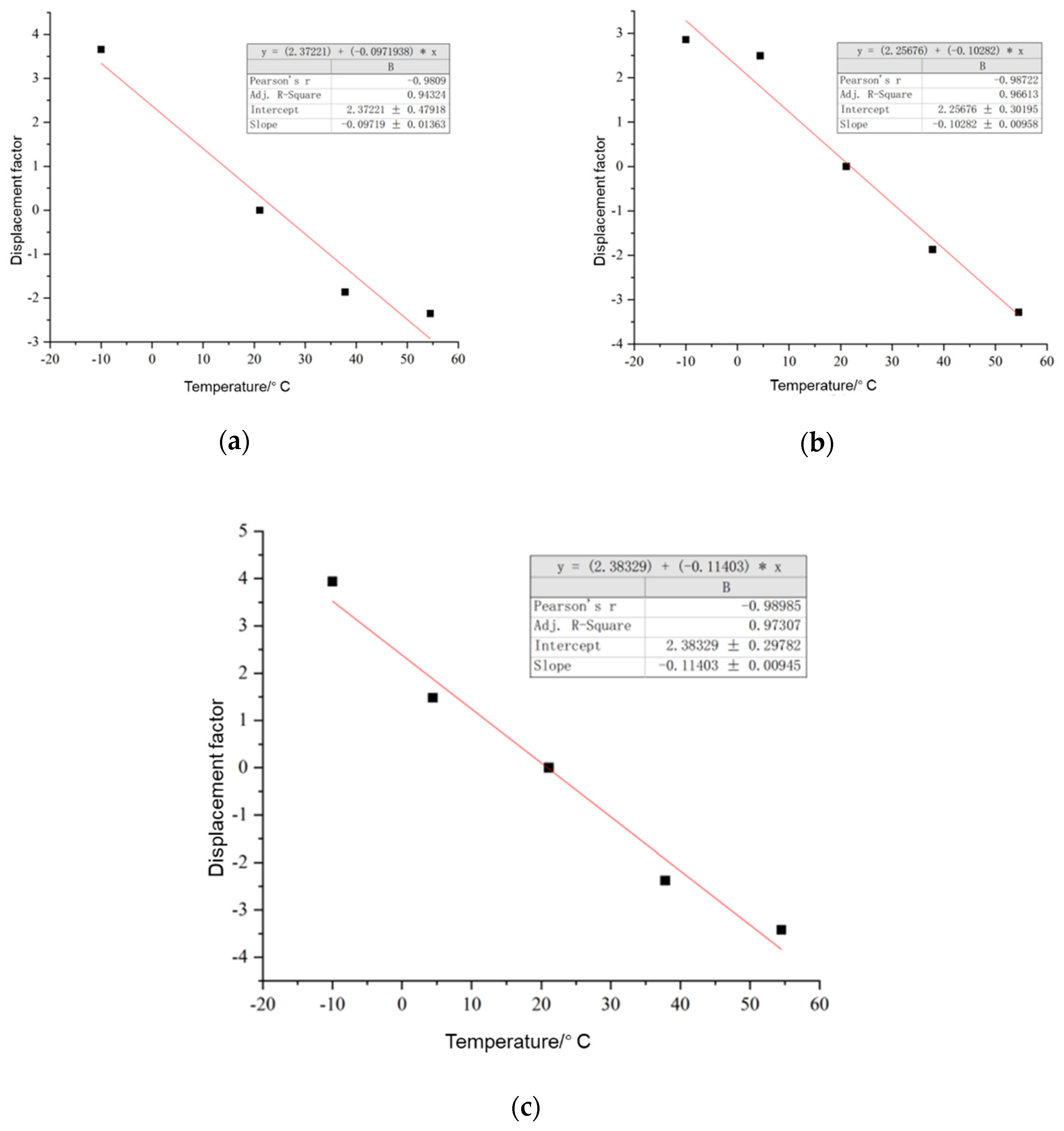
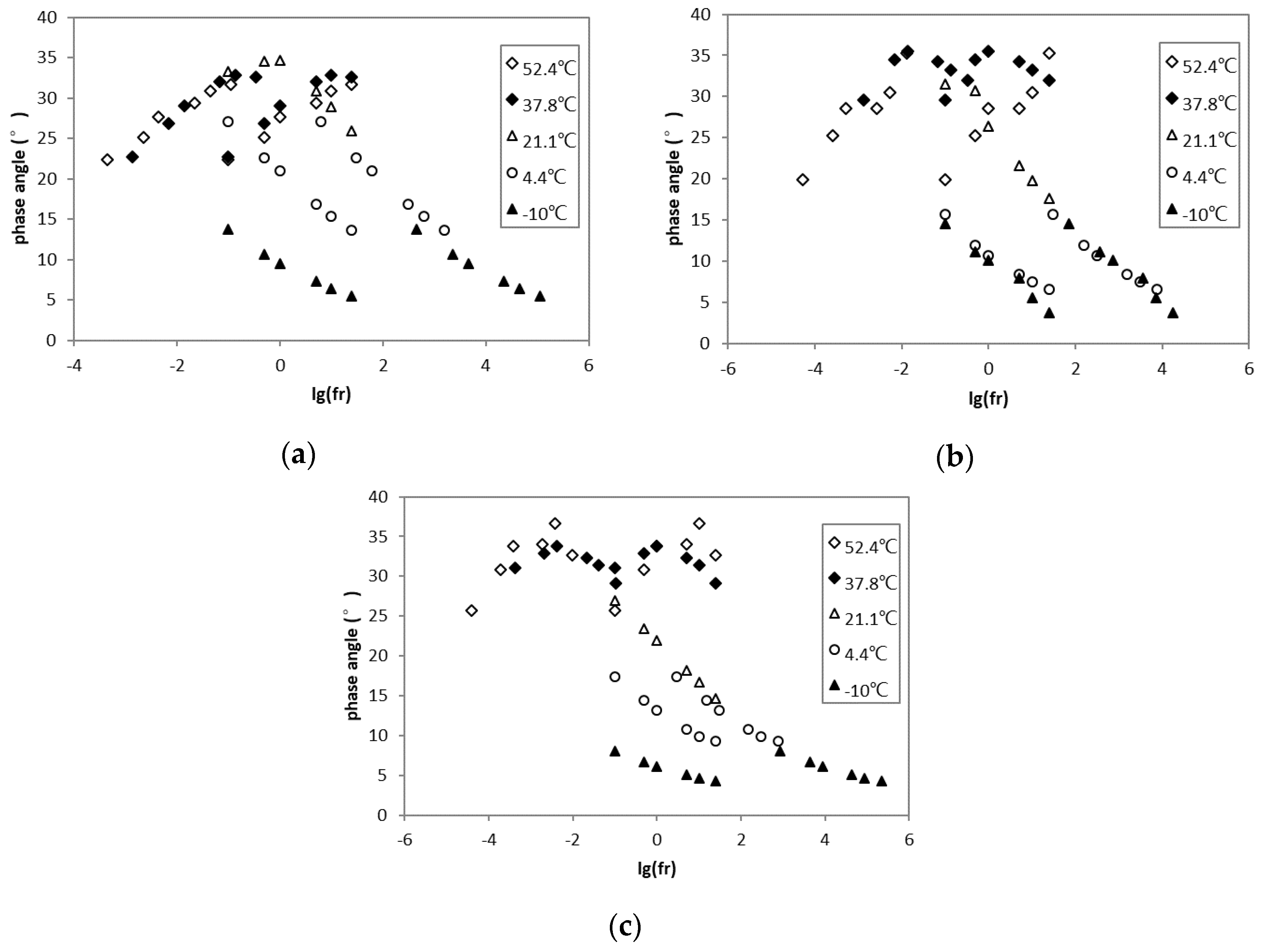
3.2.2. Viscoelastic Behavior Analysis

According to the formula, the displacement factors for the three composite pavement structures at temperatures of −10 °C, 4.4 °C, 21.1 °C, 37.8 °C, and 54.5 °C were obtained through the nonlinear programming solver in Excel software 2022. The reference temperature for these displacement factors is 21 °C, and the displacement factor for the three composite pavement structures at α(21) = 1 is shown in

Table 14. Temperature shift factors.

Temperature (°C)	3 + 3	4 + 4	6 + 4
−10	3.6562	2.8569	3.9403
4.4	1.7899	2.4934	1.4798
21.1	0	0	0
37.8	−1.8641	−1.8692	−2.3767
54.5	−2.3531	−3.2813	−3.4194

.

Figure 11 shows the displacement factors for the 3 + 3, 4 + 4, and 6 + 4 composite structures at 21.1 °C.

Based on the results in Figure 11, it can be observed that under the given conditions, the correlation coefficients between the displacement factors and temperature for the three composite structures are all greater than 0.9, indicating a good linear relationship. This linear relationship reflects the viscoelastic nature of the asphalt material.

$$\mathrm{l}\mathrm{o}\mathrm{g} {\alpha }_T=-0.097T+2.37$$

(13)

$$\mathrm{l}\mathrm{o}\mathrm{g} {\alpha }_T=-1.03T+2.26$$

(14)

$$\mathrm{l}\mathrm{o}\mathrm{g} {\alpha }_T=-0.114T+2.38$$

(15)

Performing nonlinear fitting based on the sigmoidal formula mentioned above, the four important parameters of the sigmoidal curve were obtained and are shown in

Table 15. Coefficients of the inverse function of the master curve of the complex modulus.

Type of Mixture	3 + 3	4 + 4	6 + 4
$\delta$	2.1615	1.7068	1.9487
$\alpha$	2.3658	2.8521	2.4858
$\beta$	−0.2921	−0.9956	−1.1533
$\gamma$	−0.6112	−0.5626	−0.5621

.

As mentioned earlier, |α| characterizes the amplitude of the complex modulus, indicating that the dynamic modulus amplitude variation for the three composite structures is in the range of 2.0 to 3.0. The sigmoidal curve’s minimum value, represented by the fitting parameter δ, also varies in the range of 2.0 to 3.0 for the three composite structures. Combined with Table 15, it further indicates that the maximum value of the dynamic modulus curve is around 4.5.

The main curves were plotted in a coordinate system with the reduced frequency as the abscissa and dynamic modulus and phase angle as the ordinates. Among them, Figure 12 shows the dynamic modulus master curve, while Figure 13 presents the phase angle master curve. These curves are based on experimentally measured dynamic modulus and phase angle data and are plotted in a logarithmic coordinate system, providing a better reflection of the material’s nonlinear characteristics.

From Figure 12, it can be observed that as the reduced frequency increases, the dynamic modulus gradually rises initially at a slow pace and then stabilizes at a certain frequency, forming the dynamic modulus master curve. The mechanical response characteristics exhibited by this curve can provide predictive information about the high- and low-temperature performance of asphalt mixtures. These characteristics are often difficult to directly measure in a laboratory setting, but they can be inferred from dynamic modulus values recorded at various frequencies. Therefore, the dynamic modulus master curve has become one of the key indicators for evaluating the mechanical performance of asphalt mixtures.

According to Figure 13, the phase angle of asphalt mixtures increases and then decreases with the increase in frequency, reaching a peak at a certain frequency. As the frequency approaches infinity, the phase angle approaches zero. This is because at high frequencies (low temperatures), the elastic modulus of the asphalt mixture is relatively large, and its behavior is closer to ideal elastic behavior, with stress and strain occurring almost simultaneously, resulting in a phase angle close to zero.

Based on the results from Figure 14, it can be observed that the dynamic modulus of the three composite structures exhibits a converging trend at both the high-frequency and low-frequency ends. As the frequency gradually decreases, corresponding to a continuous rise in temperature, the dynamic modulus value for the 3 + 3 structure is the lowest. In the graph, the sigmoid function master curve for the 3 + 3 structure lies below those of the 4 + 4 and 4 + 6 structures. The reduced frequency ranges for all three composite structures are relatively wide, and the converging values within the low-temperature, high-frequency range align with the conclusions mentioned earlier, with the maximum converging values being essentially similar. The main difference lies in the high-temperature, low-frequency range.

Among these three composite structures, the asphalt mixture of the 6 + 4 structure exhibits the minimum converging value for the dynamic modulus at approximately 330 MPa, while the dynamic modulus for the 3 + 3 structure has not yet reached an ideal converging state. Therefore, from the perspective of high-temperature performance, the asphalt mixture for the 6 + 4 composite structure should be prioritized as the pavement solution, with the 4 + 4 structure as the second choice.

Figure 15 displays the trends in phase angle for the three composite structures as the loading frequency varies. As the temperature gradually rises, and the frequency continuously decreases, the phase angle reaches its highest value before gradually decreasing. In the low-frequency range, the viscoelastic performance of the composite structure is outstanding, indicating that the aggregate in the composite structure begins to play a role. In the low-temperature high-frequency range, the hysteresis phenomenon in the composite structure weakens, manifested by the gradual reduction in the phase angle. In the high-temperature low-frequency range, the composite structure experiences greater resistance, demonstrating a balanced state, and the phase angle exhibits a larger value, indicating the material’s viscous behavior.

Based on the fitting results of the CAM model, the viscoelastic parameters are shown in

Table 16. Viscoelastic parameters of CAM model.

Viscoelastic Parameters	${\mathit{G}}_{\mathit{e}}^{\mathit{*}}$	${\mathit{G}}_{\mathit{g}}^{\mathit{*}}$	${\mathit{f}}_{\mathit{c}}$	${\mathit{m}}_{\mathit{e}}$	$\mathit{k}$	$\mathit{R}$	R2
3 + 3	2.60	40695	28	0.596	0.647	0.277327	0.999
4 + 4	2.73	41367	34	0.695	0.569	0.367653	0.997
6 + 4	3.10	42036	41	0.584	0.710	0.247583	0.998

.

As per Table 16, it is evident that considering the low-temperature performance indicators Gg* and $f_c$, the 6 + 4 structure consistently exhibits a higher glassy-state complex modulus ($G_g^{*}$) compared to the 3 + 3 and 4 + 4 structures. Additionally, the crossover frequency $f_c$ for the 6 + 4 structure is higher than that for the 3 + 3 and 4 + 4 structures, with the 4 + 4 structure performance being intermediate. Therefore, in terms of low-temperature performance indicators, the 6 + 4 structure appears to be the most favorable, followed by the 4 + 4 structure. Furthermore, the equilibrium complex modulus $G_e^{*}$ can serve as an indicator of high-temperature performance, and in this aspect, the equilibrium modulus for the 6 + 4 structure is consistently higher than that for the other two structures.

According to Figure 16 and considering the information from Table 16, the arrangement of crossover frequency ($f_c$) is as follows for the composite structures: 6 + 4 structure > 4 + 4 structure > 3 + 3 structure. The arrangement of the equilibrium complex modulus ($G_e^{*}$) is as follows: 6 + 4 structure > 4 + 4 structure > 3 + 3 structure. Analysis of the graphs and tables indicates that the high- and low-temperature performance of the three composite structures is related to the thickness of the composite structure. Overall, the 6 + 4 structure exhibits better high- and low-temperature performance, the 4 + 4 structure can be considered as an alternative, while the 3 + 3 structure is not recommended.

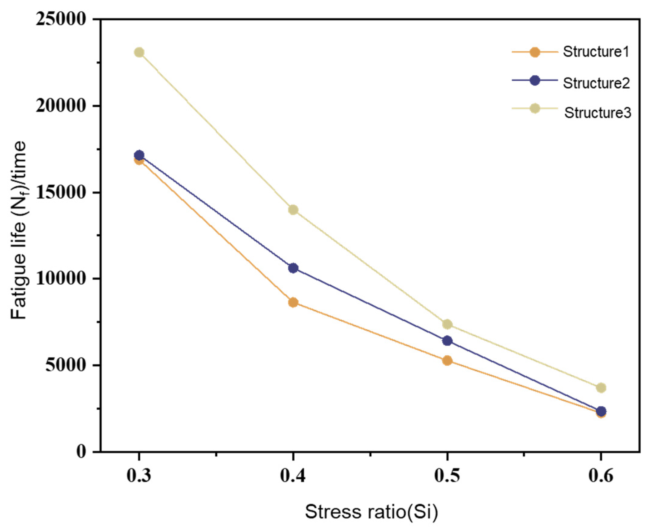
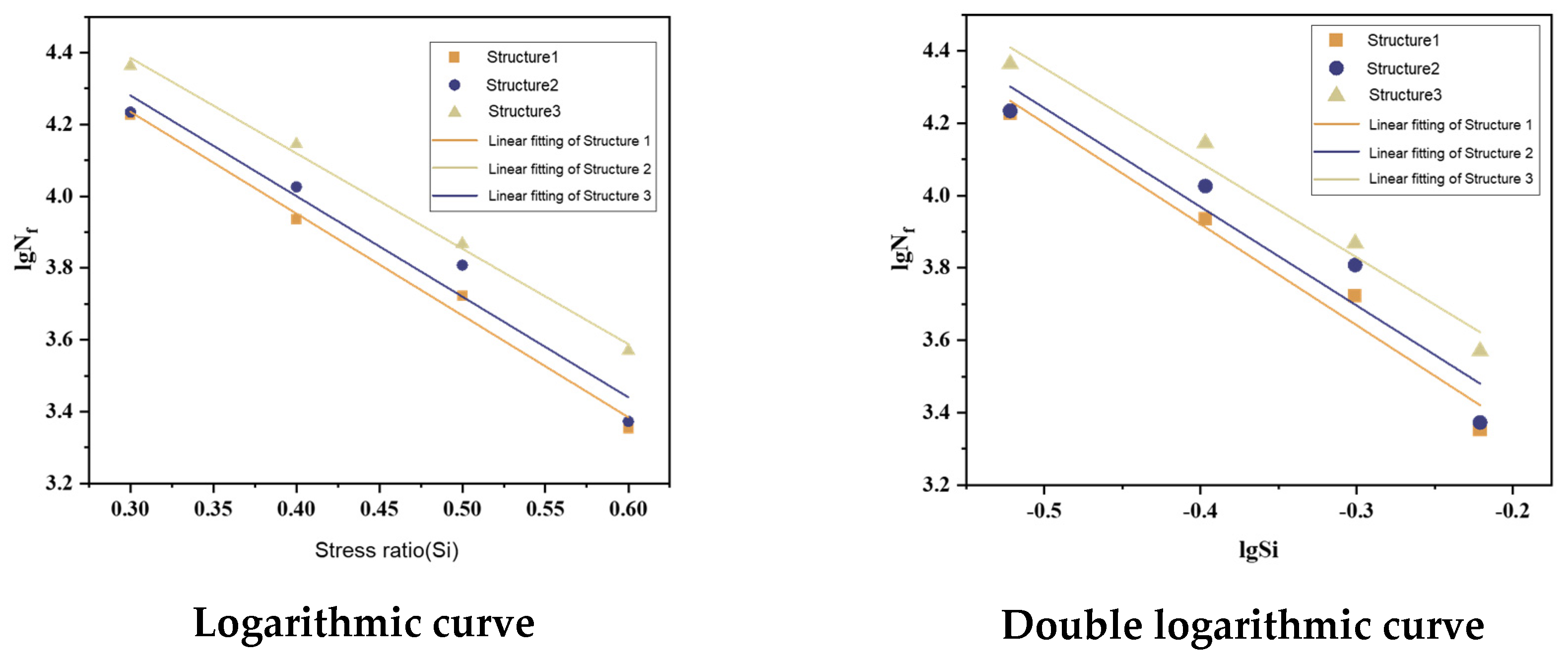
3.3. Fatigue Test Results and Analysis for High-Performance Composite Structures

In this section, four-point fatigue tests were conducted under stress control conditions with stress ratios of 0.3, 0.4, 0.5, and 0.6. Fatigue tests were performed on composite structures of SMA-13, AC-20, and SMA-10 asphalt mixtures using a four-point bending fatigue test setup. The results of the fatigue tests for different stress ratios and fatigue lives are presented in

Table 17. Fatigue life of three composite structures.

Structure Type	Stress Ratio	Fatigue Life
		1	2	3	Average Value
Structure 1	0.3	16,524	17,532	16,562	16,873
	0.4	9152	8250	8528	8643
	0.5	5652	5012	5186	5283
	0.6	1896	2521	2350	2256
Structure 2	0.3	17,128	16,925	17,367	17,140
	0.4	10,547	9654	11,683	10,628
	0.5	6781	6149	6368	6432
	0.6	1987	2645	2460	2364
Structure 3	0.3	22,679	23,025	23,529	23,078
	0.4	14,456	13,856	13,552	13,988
	0.5	6925	7362	7856	7381
	0.6	4098	3625	3425	3716

, and the relationship is illustrated in Figure 17.

Fatigue lives (N_f) and stress ratios (S_i) exhibit a linear relationship in a logarithmic coordinate system. The fatigue life under stress control conditions can be described by a logarithmic fatigue equation, as shown in Equation (16).

$$\lg N_f=K+n(\delta /S)$$

(16)

Equation definitions:

$N_f$—Fatigue life;

K, n—Regression coefficients, where k represents the intercept of the stress curve, and n is the slope of the fatigue curve;

$\delta /S$—Stress ratio.

Comparative analysis of the fatigue performance of the three different composite structures is presented by plotting fatigue life curves and single–double logarithmic curves for stress ratios, as depicted in Figure 18.

Summarizing the fitted fatigue life curves for the three different composite pavement structures, the fatigue equations are obtained and detailed in

Table 18. Fatigue life equations for three composite structures.

Composite Structure	Single Logarithmic Fatigue Life Equation	Double Logarithmic Fatigue Life
Structure 1	$\mathrm{l}\mathrm{g}\mathrm{N}\mathrm{f}=-2.83\mathrm{S}\mathrm{i}+5.08$	$\mathrm{lgNf}=-2.794\mathrm{lgSi}+2.8033$
Structure 2	$\mathrm{l}\mathrm{g}\mathrm{N}\mathrm{f}=-2.80\mathrm{S}\mathrm{i}+5.12$	$\mathrm{l}\mathrm{g}\mathrm{N}\mathrm{f}=-2.729\mathrm{g}\mathrm{S}\mathrm{i}+2.8777$
Structure 3	$\mathrm{l}\mathrm{g}\mathrm{N}\mathrm{f}=-2.66\mathrm{S}\mathrm{i}+5.18$	$\mathrm{l}\mathrm{g}\mathrm{N}\mathrm{f}=-2.613\mathrm{l}\mathrm{g}\mathrm{S}\mathrm{i}+3.0451$

.

Based on Table 18, under the same test conditions, the fatigue life equations for different stress ratios exhibit the following characteristics: In the double logarithmic equation for Structure 3, the k-value is the highest, indicating that Structure 3 has the highest fatigue life. Conversely, in the single logarithmic equation for Structure 1, the k-value is the lowest, suggesting the poorest fatigue resistance. Therefore, relative to Structures 1 and 2, the fatigue performance of composite Structure 3 is slightly better. Additionally, the fatigue performance under different stress ratios follows the order: Structure 3 > Structure 2 > Structure 1.

3.4. Rutting Test Results and Analysis for High-Performance Composite Structures

Following the method in this section, rutting test specimens were formed for three composite structures: 3 + 3, 4 + 4, and 6 + 4. The thicknesses of the rutting test specimens were set at 60 mm, 80 mm, and 100 mm. The specimens were coated with bonding oil and subjected to rutting tests at 60 °C using a wheel tracking device. The test results are presented in

Table 19. Rutting test results of composite structures.

Structural Type	Dynamic Stability (times/mm)	Standard Deviation
3 + 3	5951	256
4 + 4	6186	245
6 + 4	7881	334

, and the data are graphically depicted in Figure 19.

From Figure 19, it is observed that, for the three different composite structures (3 + 3, 4 + 4, 6 + 4), their dynamic stability shows a decreasing trend. However, compared to the other two composite structures, the dynamic stability of the 3 + 3 composite structure is superior. This implies that in a double-layer SMA composite structure, dynamic stability of the composite pavement structure can be effectively improved. This is consistent with the results of SMA rutting indicators discussed in this paper. Therefore, for the selection of high-temperature performance of composite structures, the 3 + 3 structure is the optimal choice.

4. Conclusions

Based on the detailed analysis and experimental results presented in this study, the following conclusions can be drawn:

(1)

The interlayer shear strength of composite pavement structures is influenced by the asphalt mixture used and the presence of a bonding layer. Among the tested structures, the 4 + 4 combination (4 cm SMA-13 on top + 4 cm SMA-10 below) exhibited the highest shear strength, indicating better interlayer bonding and resistance to shear failure.

(2)

The bonding energy evaluation using peak relative displacement as an indicator was found to be an effective method for assessing interlayer shear performance. This approach provided a strong correlation between bonding energy and shear strength, allowing for a more accurate evaluation of interlayer bond strength.

(3)

The dynamic modulus tests revealed that the 6 + 4 composite structure (6 cm SMA-13 on top + 4 cm AC-20 below) exhibited superior high-temperature performance compared to the other tested structures. This structure maintained a higher modulus at elevated temperatures, indicating better resistance to deformation and rutting.

(4)

The fatigue test results indicated that the 6 + 4 composite structure also performed best in terms of fatigue life. This structure demonstrated the highest fatigue resistance under different stress ratios, making it a favorable choice for applications requiring high durability.

(5)

While the 3 + 3 composite structure (3 cm SMA-10 on top + 3 cm SMA-10 below) exhibited the highest dynamic stability in the rutting tests, all tested structures met the minimum requirements for rutting resistance. However, the 6 + 4 structure, with its superior high-temperature performance, is still recommended for applications where high-temperature rutting is a concern.

(6)

Limitations and future goals: The tests were conducted under a specific set of conditions (e.g., temperatures, loading frequencies). Expanding the range of conditions tested would provide a more comprehensive understanding of the material’s behavior. Conducting additional tests with a wider range of temperatures, loading frequencies, and asphalt mixture compositions would provide a more robust evaluation of the material’s performance.

References

1. Zhang, K.; Liu, Y.; Nassiri, S.; Li, H.; Englund, K. Performance evaluation of porous asphalt mixture enhanced with high dosages of cured carbon fiber composite materials. Constr. Build. Mater. 2021, 274, 122066. [Google Scholar] [CrossRef]
2. Tian, Y.; Sun, L.; Li, H.; Zhang, H.; Harvey, J.; Yang, B.; Zhu, Y.; Yu, B.; Fu, K. Laboratory investigation on effects of solid waste filler on mechanical properties of porous asphalt mixture. Constr. Build. Mater. 2021, 279, 122436. [Google Scholar] [CrossRef]
3. Al-Qadi, I.L.; Said, I.M.; Ali, U.M.; Kaddo, J.R. Cracking prediction of asphalt concrete using fracture and strength tests. Int. J. Pavement Eng. 2022, 23, 3333–3345. [Google Scholar] [CrossRef]
4. Wang, W.; Duan, S.; Zhu, H. Research on improving the durability of bridge pavement using a high-modulus asphalt mixture. Materials 2021, 14, 1449. [Google Scholar] [CrossRef] [PubMed]
5. Ouyang, W.; Yu, G.F.; Zhu, F.F. Research on anti-rutting performance of high modulus asphalt concrete pavement. Adv. Mater. Res. 2011, 163, 4474–4477. [Google Scholar]
6. Qian, G.; Yao, D.; Gong, X.; Yu, H.; Li, N. Performance evaluation and field application of hard asphalt concrete under heavy traffic conditions. Constr. Build. Mater. 2019, 228, 116729. [Google Scholar] [CrossRef]
7. Si, C.; Zhou, X.; You, Z.; He, Y.; Chen, E.; Zhang, R. Micro-mechanical analysis of high modulus asphalt concrete pavement. Constr. Build. Mater. 2019, 220, 128–141. [Google Scholar] [CrossRef]
8. Geng, L.-T.; Xu, Q.; Ren, R.-B.; Wang, L.-Z.; Yang, X.-L.; Wang, X.-Y. Performance research of high-viscosity asphalt mixture as deck-paving materials for steel bridges. Road Mater. Pavement Des. 2017, 18, 208–220. [Google Scholar] [CrossRef]
9. Qin, X.; Zhu, S.; He, X.; Jiang, Y. High temperature properties of high viscosity asphalt based on rheological methods. Constr. Build. Mater. 2018, 186, 476–483. [Google Scholar] [CrossRef]
10. Zhou, Z.; Chen, G. Preparation, Performance, and modification mechanism of high viscosity modified asphalt. Constr. Build. Mater. 2021, 310, 125007. [Google Scholar] [CrossRef]
11. Arnold, G.; Darcy, R.; Hall, S.; Mudgway, G. High modulus asphalt to prevent rutting at intersections. In Proceedings of the 17th AAPA International Flexible Pavements Conference, Melbourne, Victoria, Australia, 13–16 August 2017; pp. 13–16. [Google Scholar]
12. Espersson, M. Effect in the high modulus asphalt concrete with the temperature. Constr. Build. Mater. 2014, 71, 638–643. [Google Scholar] [CrossRef]
13. Jin, D.; Boateng, K.A.; Chen, S.; Xin, K.; You, Z. Comparison of rubber asphalt with polymer asphalt under long-term aging conditions in Michigan. Sustainability 2022, 14, 10987. [Google Scholar] [CrossRef]
14. Jin, D.; Yin, L.; Xin, K.; You, Z. Comparison of asphalt emulsion-based chip seal and hot rubber asphalt-based chip seal. Case Stud. Constr. Mater. 2023, 18, e02175. [Google Scholar] [CrossRef]
15. Jin, D.; Yin, L.; Malburg, L.; You, Z. Laboratory evaluation and field demonstration of cold in-place recycling asphalt mixture in Michigan low-volume road. Case Stud. Constr. Mater. 2024, 20, e02923. [Google Scholar] [CrossRef]
16. Zeng, G.; Wu, W.; Li, J.; Xu, Q.; Li, X.; Yan, X.; Han, Y.; Wei, J. Comparative study on road performance of low-grade hard asphalt and mixture in China and France. Coatings 2022, 12, 270. [Google Scholar] [CrossRef]
17. Vaitkus, A.; Čygas, D.; Kleizienė, R.; Žiliūtė, L. New solutions for distressed pavement rehabilitation of Vilnius city streets. In Proceedings of the Road and Rail Infrastructure III, Split, Croatia, 28–30 April 2014. [Google Scholar]
18. Li, J.; Chai, L. A Case Study of Asphalt Pavement Overlay for Beinjing West Chang’an Avenue Using Modified Bitumen of High Viscosity and Elasticity. In Proceedings of the 2015 4th International Conference on Sensors, Measurement and Intelligent Materials, Shenzhen, China, 27–28 December 2015; Atlantis Press: Amsterdam, The Netherlands, 2016; pp. 27–278. [Google Scholar]
19. Wang, T.; Dra, Y.A.S.S.; Cai, X.; Cheng, Z.; Zhang, D.; Lin, Y.; Yu, H. Advanced cold patching materials (CPMs) for asphalt pavement pothole rehabilitation: State of the art. J. Clean. Prod. 2022, 366, 133001. [Google Scholar] [CrossRef]
20. Lu, Z.; Feng, Z.-G.; Yao, D.; Li, X.; Jiao, X.; Zheng, K. Bonding performance between ultra-high performance concrete and asphalt pavement layer. Constr. Build. Mater. 2021, 312, 125375. [Google Scholar] [CrossRef]
21. Haslett, K.E.; Robinson, Z.; Wielinski, J. Comparison of Bond Strength Evaluation Methods between Pavement Layers; Transportation Research Record: Washington, DC, USA, 2022; p. 03611981221141434. [Google Scholar]
22. Bonaquist, R.F. Simple Performance Tester for Superpave Mix Design: First-Article Development and Evaluation; Transportation Research Board: Washington, DC, USA, 2003; Volume 513. [Google Scholar]
23. Wang, T.; Li, M.; Cai, X.; Cheng, Z.; Zhang, D.; Sun, G. Multi-objective design optimization of composite polymerized asphalt emulsions for cold patching of pavement potholes. Mater. Today Commun. 2023, 35, 105751. [Google Scholar] [CrossRef]
24. Boz, I.; Tavassoti-Kheiry, P.; Solaimanian, M. The advantages of using impact resonance test in dynamic modulus master curve construction through the abbreviated test protocol. Mater. Struct. 2017, 50, 176. [Google Scholar] [CrossRef]
25. Corrales-Azofeifa, J.; Archilla, A.R.; Miranda-Argüello, F.; Loria-Salazar, L. Effects of moisture damage and anti-stripping agents on hot mix asphalt dynamic modulus. Road Mater. Pavement Des. 2020, 21, 1135–1154. [Google Scholar] [CrossRef]
26. Yuan, D.; Jiang, W.; Hou, Y.; Xiao, J.; Ling, X.; Xing, C. Fractional derivative viscoelastic response of high-viscosity modified asphalt. Constr. Build. Mater. 2022, 350, 128915. [Google Scholar] [CrossRef]
27. Zeng, M.; Bahia, H.U.; Zhai, H.; Anderson, M.R.; Turner, P. Rheological modeling of modified asphalt binders and mixtures (with discussion). J. Assoc. Asph. Paving Technol. 2001, 70, 403–441. [Google Scholar]
28. Xu, J.; Zheng, C. Random generation of asphalt mixture mesostructure and thermal–mechanical coupling analysis at low temperature. Constr. Build. Mater. 2021, 280, 122537. [Google Scholar] [CrossRef]
29. Chehab, G.; Kim, Y.; Schapery, R.; Witczak, M.; Bonaquist, R. Time-temperature superposition principle for asphalt concrete with growing damage in tension state. J. Assoc. Asph. Paving Technol. 2002, 71, 559–593. [Google Scholar]
30. Dondi, G.; Pettinari, M.; Sangiorgi, C.; Zoorob, S.E. Traditional and Dissipated Energy approaches to compare the 2PB and 4PB flexural methodologies on a Warm Mix Asphalt. Constr. Build. Mater. 2013, 47, 833–839. [Google Scholar] [CrossRef]
31. Shafabakhsh, G.; Rajabi, M. The fatigue behavior of SBS/nanosilica composite modified asphalt binder and mixture. Constr. Build. Mater. 2019, 229, 116796. [Google Scholar] [CrossRef]
32. JTG E20-2011; Specifications and Test Methods of Bitumen and Bituminous Mixtures for Highway Engineering. China Communication Press: Beijing, China, 2011.
Figure 1. Schematic diagram of bond energy calculation.
Buildings 14 01885 g001
Figure 2. Dynamic modulus test.
Buildings 14 01885 g002
Figure 3. Four-point fatigue test device.
Buildings 14 01885 g003
Figure 4. Composite beam specimen.
Buildings 14 01885 g004
Figure 5. Relationship between shear strength and pavement structure.
Buildings 14 01885 g005
Figure 6. Shear–relative displacement curves of four asphalt mixtures.
Buildings 14 01885 g006
Figure 7. Shear strength–bond energy relationship curve.
Buildings 14 01885 g007
Figure 8. Shear–displacement curve of composite structure.
Buildings 14 01885 g008
Figure 9. Shear strength–bonding energy relationship curve.
Buildings 14 01885 g009
Figure 10. Dynamic modulus of composite pavements at 10 Hz.
Buildings 14 01885 g010
Figure 11. Shift factor at 21.1 °C, (a) 3 + 3; (b) 4 + 4; (c) 6 + 4.
Buildings 14 01885 g011
Figure 12. Master curves of dynamic modulus of asphalt with three composite structures, (a) 3 + 3 dynamic modulus master curve; (b) 4 + 4 dynamic modulus master curve; (c) 6 + 4 dynamic modulus master curve.
Buildings 14 01885 g012
Figure 13. Main curve of phase angle of asphalt for three composite structures, (a) 3 + 3 phase angle master curve; (b) 4 + 4 phase angle master curve; (c) 6 + 4 phase angle master curve.
Buildings 14 01885 g013
Figure 14. Master curves of dynamic modulus of three composite structures.
Buildings 14 01885 g014
Figure 15. Phase angle master curve of three composite structures.
Buildings 14 01885 g015
Figure 16. Modulus master curve of CAM model.
Buildings 14 01885 g016
Figure 17. Relationship between stress ratios and fatigue life of different composite structures.
Buildings 14 01885 g017
Figure 18. Logarithmic curves for different composite structures.
Buildings 14 01885 g018
Figure 19. Dynamic stability of composite structures.
Buildings 14 01885 g019