Derivation and Application of Analytical Coupling Loss Coefficient by Transfer Function in Soil–Building Vibration

Abstract

Vibrations generated by railways may undergo amplification or reduction while traversing the foundations, floors, and spans of adjacent structures. This fluctuation in the vibration intensity, identified as a building’s coupling loss, is commonly considered in vibration forecasts through the utilization of universal frequency-independent adjustment parameters. This article employs a theoretical analytical approach to investigate the propagation characteristics of Rayleigh waves in elastic foundation soil, as well as the variations at the contact surface of buildings’ foundations. Analytical expressions for the coupling loss coefficient are derived to explore the displacement transfer relationship in the soil–structure interaction. To accurately and efficiently analyze the proposed buildings and site, the entire vibration propagation system is decoupled into substructure systems for independent analytical calculations. Theoretical analytical methods are utilized to obtain the displacement transfer functions between the soil and the structures through the refraction and transmission of waves. From a theoretical perspective, a thorough understanding of the interaction between soil and buildings is achieved. The influence of various variables related to railways and foundations on the building responses is analyzed. By comparing with measured data, the correctness of the analytical form of the coupling loss coefficient is validated, filling a gap in the literature due to the lack of analytical research on displacement transfer losses in soil–structure interactions.

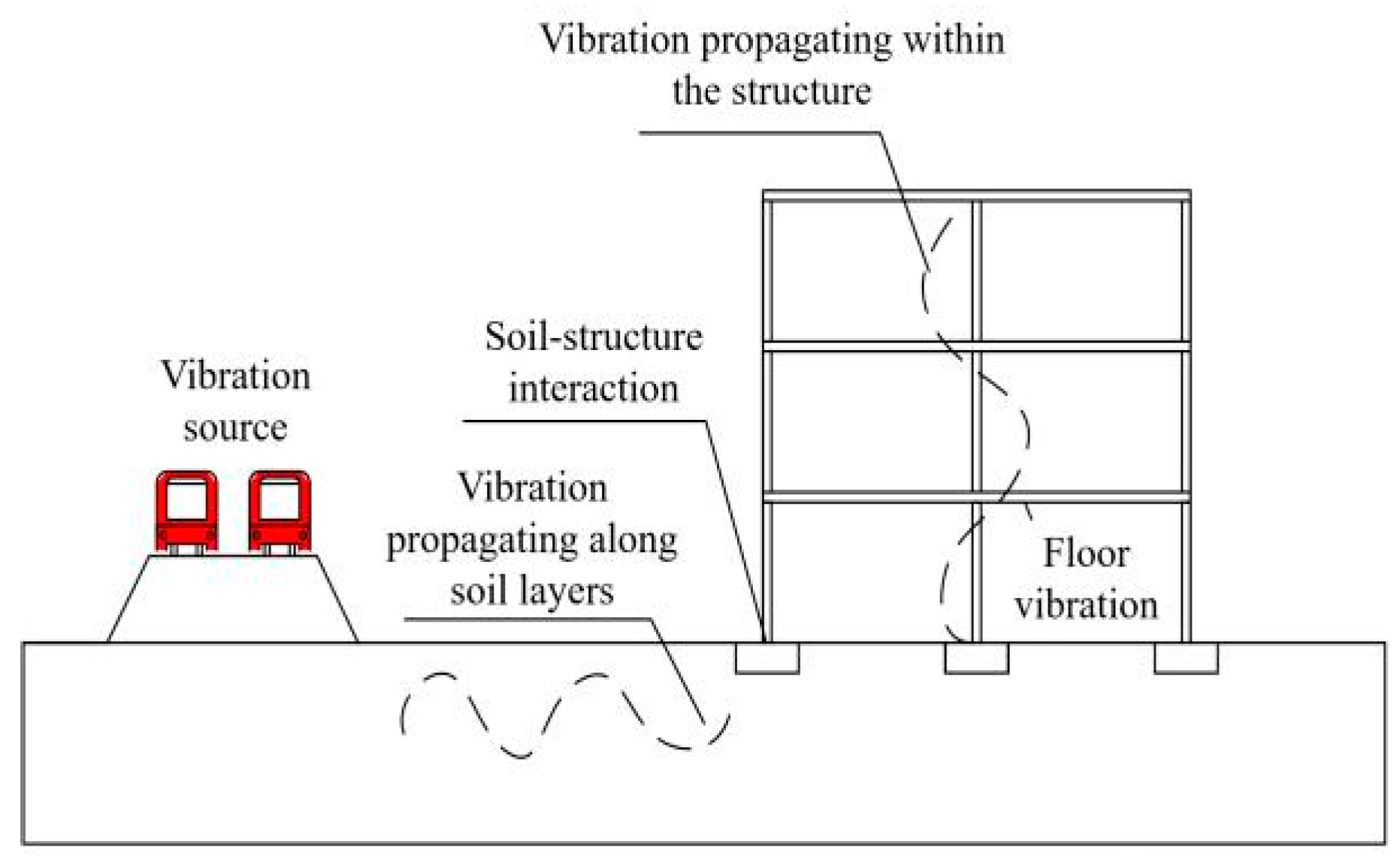
1. Introduction

The propagation of vibrations generated by railway systems can significantly impact the structural integrity and comfort levels of adjacent buildings. These vibrations, which may amplify or attenuate as they travel through soil and building foundations, are quantified by the coupling loss coefficient, a critical factor when predicting and managing building responses to environmental vibrations.

In the 1960s and 1970s, the gradual development of high-speed railways emerged as a convenient and efficient transportation infrastructure in developed countries. A significant focus of scholarly inquiry during this period involved the examination of the environmental vibration responses induced by rail transit. In 1850, Professor Krylov et al. [1,2,3] in the United Kingdom pioneered the establishment of a ground vibration prediction model, basing it on the dynamic loads derived from vehicle loads. Utilizing the classical Green function equation, their work delved into the study of ground vibration responses resulting from rail transit. In 1970, Lang and Kurzweil [4] contributed a predictive Equation for train-induced vibrations through extensive research, correlating the vibration levels and distances with low-frequency vibrations. In 1988, Takemiya Hirokazu [5] employed a quasi-static method to analyze the vibration response of the Shinkansen track system caused by high-speed trains. This comprehensive analysis included the examination of viaduct and pile foundation vibrations. Takemiya studied the resistance surrounding the vibration source and the influence of layered soil on elastic wave propagation in the foundation soil, and then proposed a damping scheme. By comparing three different arrangements encompassing diverse materials, damping effects, and wave damping zones, the optimal damping effect was determined.

In 2020, Yue Jianyong et al. [6] employed a test method to measure the tunnel and surrounding building accelerations before and after subway vibration reduction. This facilitated the analysis and evaluation of subway vibration reduction effects. Building on this, a finite element and infinite element coupling numerical simulation method was employed to simulate the vibration response of surrounding buildings during subway operations. The resulting vibration characteristics were then compared with measured data. Fang Lei’s work in 2020 [7] involved simulating soil–structure interaction through the derivation of the stiffness coefficients between soil and building. Additionally, an enhancement to the prediction model’s accuracy was achieved through the application of the random forest algorithm. In 2021, Colaco et al. [8,9,10] predicted the vibration generation and propagation in the track–ground–building system using the 2.5DFEM-MFS method for tracks and the 3DFEM method for buildings. In the same year, Sadeghi et al. [11,12,13] established and verified a vibration acoustic model for buildings based on field test results. The building parameters were categorized based on the structural and non-structural characteristics, and a model parameter analysis was conducted to study the influence of the building structural and acoustic parameters on structural noise. The derived prediction model facilitated establishing the functional relationship between train-induced vibration acceleration and buildings. In 2021, Yasser E. Ibrahim et al. [14] conducted a detailed three-dimensional finite element analysis of a 10-story reinforced concrete frame structure based on a raft, utilizing ABAQUS 2020. The study, employing a moving point load to simplify the train load, investigated the effects of the train speed and the distance between the train and the building on the vibration response of the foundation structure. The research concluded that the use of open ditches and filled foam ditches mitigated the vibration response induced by trains.

Presently, the numerical simulation method necessitates simplifications and assumptions within the overall finite element model, compromising the accuracy of the calculation results. Although the test methods yield accurate and reliable results, they are time-consuming and expensive. The test method is also susceptible to external factors, such as the environmental conditions, sensor instability, and background noise, introducing interference to the test data and thereby imposing limitations on the derived prediction equations. In light of these considerations, this study derives the coupling loss coefficient of an elastic soil foundation through theoretical analysis.

2. Theoretical Study of the Transfer Function Method

During the operation of a high-speed train, the vibrations generated by the interaction between the train and the track propagate through the roadbed to the surrounding soil and buildings, giving rise to a vibration transmission system involving the train, subgrade, foundation soil, building foundation, and the building itself, as depicted in Figure 1. The ISO14837-1 standard [15] defines the frequency domain function expression A(f) for building vibration, consisting of the source term S(f), the propagation term P(f), and the receiving term R(f). The magnitude of the building vibration A(f) is mathematically represented as A(f) = S(f)P(f)R(f). Consequently, employing the transfer function method, the entire vibration propagation system is decomposed into sub-structural systems for independent analysis and calculation (Equation (1)). These sub-structural systems include the train–track–site soil system (refer to Figure 2), soil–structure dynamic interaction system (refer to Figure 3), and building structural system (refer to Figure 4).

$$U_b\left(f\right)={U_0}^{soil}\left(f\right)\cdot C_l\left(f\right)\cdot F_a\left(f\right)$$

(1)

Equation (1) represents the calculation equation for the transfer function method. Examining the equation, it becomes evident that the vibration response, U₀^soil, of the free field comprises the vibration source term, S(f), and the propagation term, P(f). Simultaneously, the receiving term, R(f), comprises the coupling loss coefficient, C_l, and the floor amplification coefficient, F_a. Notably, the floor amplification factor is solely determined by the structural form and material characteristics of the building. To elaborate, once the inherent properties, such as the structural form of the building, are established, the floor amplification factor is determined accordingly. Consequently, the acceptance term, R(f), is solely dependent on the coupling loss coefficient, C_l. This paper focuses on the investigation of the reflection and transmission law of Rayleigh waves propagating through the building foundation. The relationship between incident waves, reflected waves, and transmitted waves is thoroughly analyzed. Subsequently, the coupling loss coefficient of the soil–structure transfer function is derived at the contact surface between the soil and the structure. This approach eliminates the need for a complex modeling process and measurement methods, ensuring both efficiency and accuracy in the calculation process.

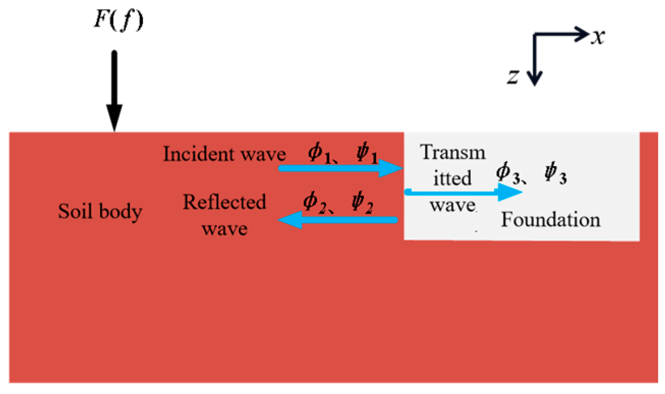
2.1. Propagation Law of Rayleigh Waves

The propagation of waves through elastic materials is subject to geometric damping, where, following the principle of the conservation of energy, the amplitude of the wave gradually decreases with increasing wave intensity and diffusion. Miller [16] was the first to characterize the wave field under a concentrated load. Importantly, the acceptance term, R(f), is exclusively determined by the coupling loss coefficient, C_l [17].

Consequently, in incorporating the soil–structure interaction into the process of resolving the vibration response of a building, the floor amplification factor is determined subsequent to establishing the building’s form. The determination of the floor amplification factor is integral to comprehensively understanding and applying the soil–structure interaction in the context of solving building vibration responses. On the free interface, when the incidence angle of the SV wave is substantial, a Rayleigh surface waveform manifests on the free interface, propagating along it with its amplitude diminishing as the distance from the interface increases. While there are alternative methods for generating Rayleigh surface waves, in a half space containing layered media, considering the free surface boundary conditions, interlayer continuity, and amplitude limits of an infinite domain, two distinct types of special solutions to waves emerge. One is confined solely within the half space containing layered media, while the other extends beyond the plane. Both categories of special solutions propagate along the free surface, with their amplitudes gradually decreasing to zero at greater depths. These special solutions are identified as Rayleigh surface waves and Love surface waves.

The decay of the vibration is influenced by the properties of the medium and increases with the vertical distance. When the vertical distance is infinite, the displacement tends toward zero, indicating that Rayleigh waves exclusively propagate on the soil surface [18]. While surface waves propagate along the free surface, the energy of body waves not only travels along the free surface but also diffuses deeply within the medium. Consequently, the amplitude of surface waves decays at a much slower rate than that of body waves. Given that Rayleigh waves contribute to over two-thirds of environmental vibration during the propagation process, an examination of the attenuation characteristics of Rayleigh waves aids in understanding the laws governing vibration propagation. Consequently, this paper exclusively focuses on studying the propagation and attenuation of Rayleigh waves.

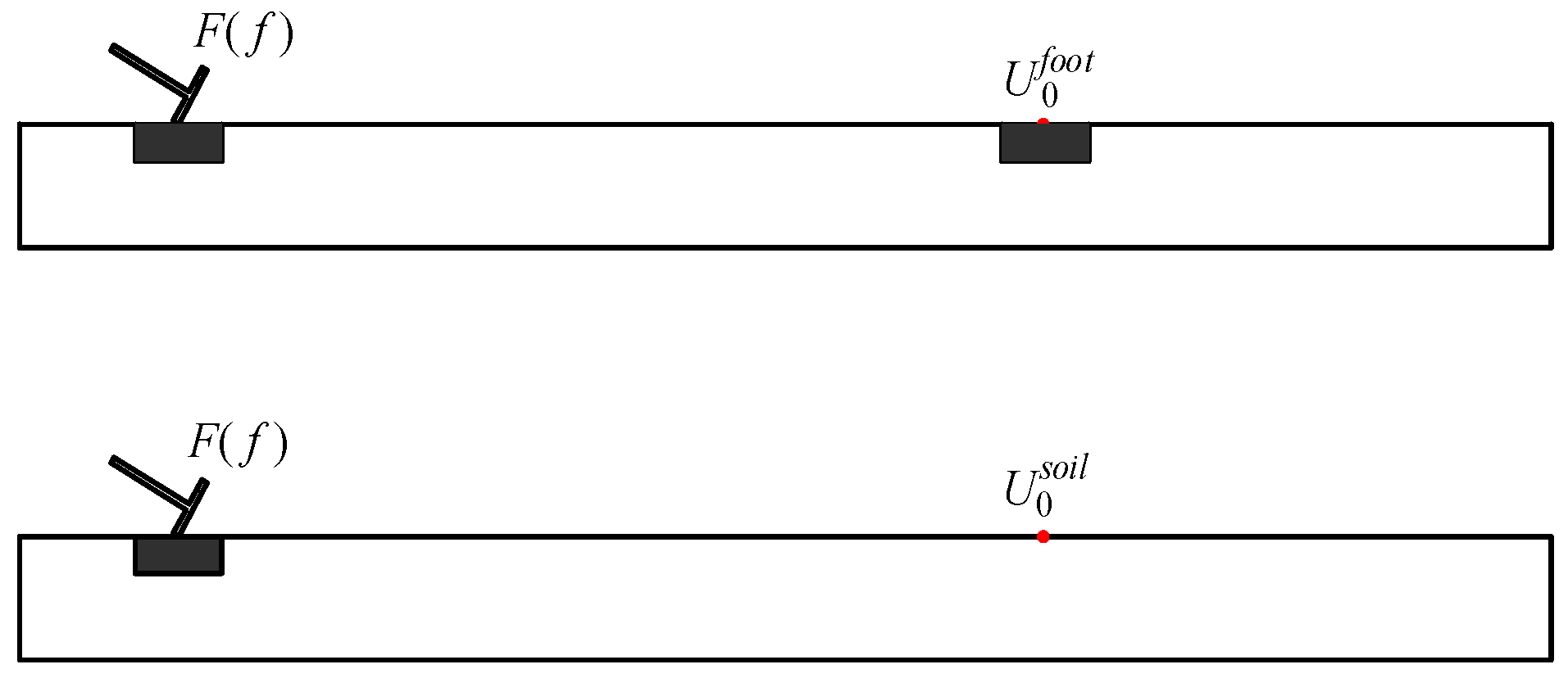
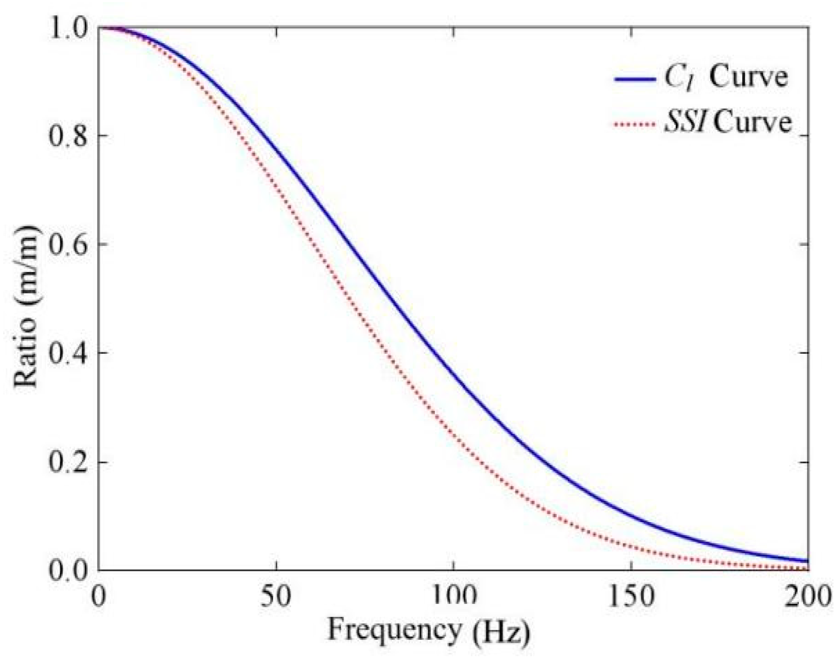
2.2. Equation Derivation of Coupling Loss Coefficients

Currently, there is a deficiency in the theoretical research on the propagation of Rayleigh waves in discontinuous media, both domestically and internationally. Previous efforts have predominantly relied on numerical methods, yielding specific outcomes. The determination of the amplitude and angle of reflected and refracted waves generated by P-waves and S-waves at the discontinuities of two media is achieved through precise consideration of six boundary conditions at these interfaces.

However, owing to the unique nature of Rayleigh waves, the amplitude of the wave mode transition from surface wave to body wave is also contingent upon the angle formed by the interface of the medium. Simply addressing the reflection and refraction of Rayleigh waves does not fully satisfy the requisite boundary conditions. Consequently, whether it is a reflected or transmitted Rayleigh wave, the mathematical challenges are more intricate, and the analytical methods are more demanding.

In 1961, Lapwood [19] delved into the reflection and transmission of Rayleigh waves at specific angles, presenting theoretical conclusions. Building on these findings, Maurice James [20] conducted an in-depth study on the reflection and transmission of Rayleigh waves. The foundational concept in Maurice James’ work is that the residual difference between the corresponding stress and displacement on either side of the contact surface should be zero. Given the intricate waveform transformations of Rayleigh waves at interfaces, including their potential transformation into Love waves or Stoneley waves, achieving this residual condition is challenging. Jafar, Zarastvand and Zhou [21] developed an analytical model to determine the sound transmission loss of a doubly curved sandwich shell with various truss core configurations.

Recent studies on building vibrations from train operations highlight key advancements. Qiu et al. [22] and Hu et al. [23] developed models for predicting and mitigating vibrations in elevated metro depots and over-track buildings, validated by field measurements. He and Tao [24] created a prediction method for urban environments, considering soil–structure interactions. Ma et al. [25] proposed a semi-analytical model for underground train-induced vibrations, validated in the Hefei metro. These studies underscore the importance of predictive modeling and validation in designing effective vibration mitigation strategies for improved urban living conditions.

While the residual cannot feasibly reach zero if Rayleigh waves only assume transmission or reflection forms, Maurice James proposed the selection of suitable transmission and reflection coefficients to minimize the relevant equation. This approach aims to bring the residual as close as possible to the zero condition, acknowledging the complexity of Rayleigh wave transformations and providing a pragmatic solution to enhance the accuracy of theoretical considerations.

$$\begin{array}{l}{I}_0=\frac{1}{I_1}{\displaystyle {\int }_0^{\infty }\left\{{\left|{\sigma }_{xx}-{\sigma }_{xx}^{\prime }\right|}^2+{\left|{\tau }_{xx}-{\tau }_{xx}^{\prime }\right|}^2\right\}}dz\\ \hspace{1em}\hspace{0.17em}\hspace{0.17em}\hspace{0.17em}+\frac{1}{I_2}{\displaystyle {\int }_0^{\infty }\left\{{\left|u-u^{\prime }\right|}^2+{\left|w-w^{\prime }\right|}^2\right\}}dz=0\end{array}$$

(2)

In Equation (2), σ_xx, σ′_xx, τ_xz, τ_xz′, u, u′, and w, w′ are the normal stresses, shear stresses, vertical displacements and horizontal displacements in the two different media, respectively. The residual I₀ represents the disparity between stress and displacement at the interface, while I₁ and I₂ denote integral expressions of stress and displacement, respectively. These expressions in Equation (3) specifically account for the contributions solely arising from the incident Rayleigh waves at the medium’s discontinuity.

$$\begin{array}{l}{I}_1={\displaystyle {\int }_0^{\infty }\left\{{\left|{\sigma }_{xx0}\right|}^2+{\left|{\tau }_{xz0}\right|}^2\right\}}dz\\ I_2={\displaystyle {\int }_0^{\infty }\left\{{\left|u_0\right|}^2+{\left|w_0\right|}^2\right\}}dz=0\end{array}$$

(3)

where σ_xxo, τ_xzo, u_o, and w_o are the normal stresses, shear stresses, vertical displacements and horizontal displacements at the interface position, respectively.

The illustration in Figure 5 depicts the propagation of Rayleigh waves on the discontinuous surface of a quarter-space medium.

After simplification, the expression for I₀ is obtained:

$$\begin{array}{l}{I}_0=\left(A+J\right){\left(1+R\right)}^2+\left(B+G\right){\left(1-R\right)}^2+\left(F+I\right)T\left(1-R\right)\\ \hspace{1em}+\left(C+E+H+K\right)T^2+\left(D+L\right)T\left(1+R\right)\end{array}$$

(4)

In Equation (4), the functions designated by the letters A to L are solely dependent on two media parameters, which can be computed to fixed values. Consequently, within the equation, only R and T remain as the two unknowns.

To minimize the value of I₀, the reflection coefficient R and transmission coefficient T can finally be calculated and determined by $\frac{\partial I_0}{\partial R}=0,\frac{\partial I_0}{\partial C}=0$.

During the simplification of the equation, the wave circular frequency ω is factored out, and as a result, the widely used transmission coefficient R and reflection coefficient T are only affected by the elastic modulus on both sides of the medium. This is significant because the expression for these coefficients is not limited to simple harmonic waves but can be extended to non-periodic waveforms as well. Any wave, through the Fourier transform, can be decomposed into the superposition of several simple harmonic waves. Each of these simple harmonic waves possesses reflection and transmission coefficients that are independent of the circular frequency. Consequently, the integrals of these simple harmonic waves also have reflection and transmission coefficients that are irrelevant to the circular frequency.

When Rayleigh waves interact with a quarter space, the primary outcomes include the generation of reflected Rayleigh waves (ψ₂, φ₂) and refracted Rayleigh waves (ψ₃, φ₃). Specifically, ψ₁ and φ₁ represent vertically incident waves originating from the positive direction of the x-axis toward the interface between the building foundation and the soil mass (at x = 0). Relevant expressions can be listed from Equations (5) to (7):

$${\psi }_1=A{{}_{1}e}^{-rz}{e}^{i(wt-k_{r}x)},{\phi }_1=B{{}_{1}e}^{-sz}{e}^{i(wt-k_{r}x)}$$

(5)

$${\psi }_2=A{{}_{2}e}^{-rz}{e}^{i(wt+k_{r}x)},{\phi }_2=B{{}_{2}e}^{-sz}{e}^{i(wt+k_{r}x)}$$

(6)

$${\psi }_3=A{{}_{3}e}^{-r^{\prime }z}{e}^{i(wt-{k_r}^{\prime }x)},{\phi }_3=B{{}_{3}e}^{-s^{\prime }z}{e}^{i(wt-{k_r}^{\prime }x)}$$

(7)

where A₁~A₃ and B₁~B₃ are constants, while φ₁, φ₂, φ₃ and Ψ₁, Ψ₂, Ψ₃ are the wave potential functions of incident wave, reflected wave and transmitted wave in two different medias, respectively.

According to the boundary conditions, the left-travelling wave B_i = −b·A_i/(2ik_rs) and the right-travelling wave B_i = b·A_i/(2ik_rs), where (i = 1, 2, 3).

The stress and displacement on the left side of the axis x = 0 can be expressed in the following Equations from (8) to (11):

$$u=\frac{\partial \phi }{\partial x}-\frac{\partial \varphi }{\partial \mathrm{z}}=i{k}_r\left(A_1-A_2\right)\left(\frac{2sr}{b}{e}^{-sz}-e^{-rz}\right)$$

(8)

$$w=\frac{\partial \phi }{\partial z}+\frac{\partial \varphi }{\partial \mathrm{x}}=-r\left(A_1+A_2\right)\left(-\frac{2k_r^2}{b}{e}^{-sz}+e^{-rz}\right)$$

(9)

$$\begin{array}{l}{\sigma }_{xx}=\lambda \left(\frac{\partial w}{\partial x}+\frac{\partial u}{\partial \mathrm{z}}\right)+\mu \frac{\partial u}{\partial x}\\ \hspace{1em}\hspace{0.17em}\hspace{0.17em}=-\mu \left(A_1+A_2\right)\left(-b{e}^{-sz}+a{e}^{-rz}\right)\end{array}$$

(10)

$$\begin{array}{l}{\tau }_{xz}=\mu \left(\frac{\partial w}{\partial x}+\frac{\partial u}{\partial \mathrm{z}}\right)\\ \hspace{1em}\hspace{0.17em}=2\mu ir{k}_r\left(A_1-A_2\right)\left(-e^{-sz}+e^{-rz}\right)\end{array}$$

(11)

where λ and μ are the Lame constants of elastic medium one.

The stress and displacement on the right side of the axis x=0 can be expressed in the following Equations from (12) to (15):

$$u^{\prime }=i{k}_r^{\prime }\left(A_3-A_4\right)\left(\frac{2s^{\prime }{r}^{\prime }}{b}{e}^{-s^{\prime }z}-e^{-r^{\prime }z}\right)$$

(12)

$$w^{\prime }=-r^{\prime }\left(A_3+A_4\right)\left(-\frac{2k_r^{\prime 2}}{b}{e}^{-s^{\prime }z}+e^{-r^{\prime }z}\right)$$

(13)

$${\sigma }_{xx}^{\prime }=-{\mu }^{\prime }\left(A_3+A_4\right)\left(-b^{\prime }{e}^{-s^{\prime }z}+a^{\prime }{e}^{-r^{\prime }z}\right)$$

(14)

$${\tau }_{xz}^{\prime }=2\mu ir{k}_r\left(A_3-A_4\right)\left(-e^{-s^{\prime }z}+e^{-r^{\prime }z}\right)$$

(15)

where the parameters with the superscript symbol ′ represent the parameters of medium two, which have the same meaning as the parameters in medium one.

The residual expression of stress and displacement caused by incident Rayleigh waves on both sides of the interface x = 0 are:

$$\begin{array}{l}{u}_0=i{k}_r{A}_1(\frac{2sr}{b}{e}^{-sz}-e^{-rz})\\ w_0=-r{A}_1(-\frac{2{k_r}^2}{b}{e}^{-sz}+e^{-rz})\\ {\sigma }_{xx0}=-\mu A_1(-b{e}^{-sz}+a{e}^{-rz})\\ {\tau }_{xz0}=2\mu ir{k}_r{A}_1(e^{-sz}-e^{-rz})\end{array}$$

(16)

Among them,

$$\begin{array}{l}{s}^2={k_r}^2-{k_{\beta }}^2,b^2=2r^2+{k_{\beta }}^2\\ k_{\alpha }=\frac{w}{c_p},k_{\beta }=\frac{w}{c_s},k_r=\frac{w}{c_R}\end{array}$$

(17)

The above equations are put into Equations (2)–(8), and in order to minimize I₀, $\frac{\partial I_0}{\partial R}=0,\frac{\partial I_0}{\partial T}=0$ is defined. The reflection coefficient R and transmission coefficient T can be expressed as:

$$R=\frac{A_2}{A_1}=\frac{X-U}{V-Y}$$

(18)

$$T=X+YR$$

(19)

Among them,

$$\begin{array}{l}X=\frac{-(D+L+F+I)}{(C+E+H+K)},Y=\frac{-(D-L+F+I)}{2(C+E+H+K)}\\ U=\frac{-(A+J-B-G)}{(F+I-D-L)},V=\frac{2(A+J+B+G)}{(F+I-D-L)}\end{array}$$

(20)

The expressions from A to L are deduced in the following Equations from (21) to (34).

$$A=\frac{{\left(c-b\right)}^2}{{\alpha }_0}$$

(21)

$$B=\frac{1}{{\alpha }_0}\frac{b^{2}r}{s}\left[\frac{1}{2r}+\frac{1}{2s}-\frac{2}{r+s}\right]$$

(22)

$$C=\frac{1}{{\alpha }_0}{\left(\frac{{\mu }^{\prime }}{\mu }\right)}^2\left[\frac{a^{\prime 2}}{2r^{\prime }}+\frac{b^{\prime 2}}{2s^{\prime }}-\frac{2a^{\prime }{b}^{\prime }}{r+s}\right]$$

(23)

$$D=-\frac{2}{{\alpha }_0}\left(\frac{{\mu }^{\prime }}{\mu }\right)\left[\frac{a^{\prime }a}{r+r^{\prime }}+\frac{b^{\prime }b}{s+s^{\prime }}-\frac{a^{\prime }b}{r^{\prime }+s}-\frac{a{b}^{\prime }}{r+s^{\prime }}\right]$$

(24)

$$E=\frac{1}{{\alpha }_0}{\left(\frac{{\mu }^{\prime }}{\mu }\right)}^2\frac{b^{2}r}{s}\left[\frac{1}{2r^{\prime }}+\frac{1}{2s^{\prime }}-\frac{2}{r^{\prime }+s^{\prime }}\right]$$

(25)

$$F=-\frac{8}{{\alpha }_0}\left(\frac{{\mu }^{\prime }}{\mu }\right)k_r^{\prime }{k}_r{r}^{\prime }r\left[\frac{1}{r+r^{\prime }}+\frac{1}{s+s^{\prime }}-\frac{1}{r^{\prime }+s}-\frac{1}{r+s^{\prime }}\right]$$

(26)

$$G=\frac{{k_r}^2}{{\beta }_0}\left[\frac{1}{2r}+\frac{2s{r}^2}{b^2}-\frac{4sr}{b(r+s)}\right]$$

(27)

$$H=\frac{-2{k_r}^{\prime }{k}_r}{{\beta }_0}\left[\frac{1}{2r^{\prime }}+\frac{2s{r}^2}{{b^{\prime }}^2}-\frac{4s^{\prime }{r}^{\prime }}{b^{\prime }(r^{\prime }+s^{\prime })}\right]$$

(28)

$$\begin{array}{l}I=\frac{-2{k_r}^{\prime }{k}_r}{{\beta }_0}[\frac{1}{r+r^{\prime }}+\frac{4s{s}^{\prime }r{r}^{\prime }}{b{b}^{\prime }\left(s+s^{\prime }\right)}\\ \hspace{1em}\hspace{0.17em}-\frac{2sr}{b(r^{\prime }+s)}-\frac{2s^{\prime }{r}^{\prime }}{b^{\prime }(r+s^{\prime })}]\end{array}$$

(29)

$$J=\frac{r^2}{{\beta }_0}\left[\frac{1}{2r}+\frac{2{k_r}^4}{b^{2}s}-\frac{4{k_r}^2}{b(r+s)}\right]$$

(30)

$$M=\frac{{r^{\prime }}^2}{{\beta }_0}\left[\frac{1}{2r^{\prime }}+\frac{2{{k^{\prime }}_r}^4}{{b^{\prime }}^2{s}^{\prime }}-\frac{4{{k^{\prime }}_r}^2}{b^{\prime }(r^{\prime }+s^{\prime })}\right]$$

(31)

$$\begin{array}{l}L=\frac{-2r^{\prime }r}{{\beta }_0}[\frac{1}{r+r^{\prime }}+\frac{4{k^{{\prime }^2}}_r{k^2}_r}{b{b}^{\prime }\left(s+s^{\prime }\right)}\\ \hspace{1em}\hspace{0.17em}-\frac{2{k^2}_r}{b(r^{\prime }+s)}-\frac{2{{k^{\prime }}^2}_r}{b^{\prime }(r+s^{\prime })}]\end{array}$$

(32)

$${\alpha }_0=\frac{a^{2}s+b^{2}r}{2rs}+\frac{s^{2}b+b^{2}r}{2s^2}-\frac{2abs+2b^{2}r}{s(r+s)}$$

(33)

$${\beta }_0=\frac{{k^2}_r+r^2}{2r}+\frac{br}{2s^2}-\frac{b}{s}$$

(34)

Given the considerable distance between the building foundation and the point of the vibration source, along with the substantial magnitude difference between the soil and the stiffness value of the building foundation, it is assumed that after the incidence of Rayleigh waves on the building foundation, the foundation undergoes rigid motion, resulting in equal vertical displacements everywhere. Therefore, the vertical displacements are denoted as U₀^foot = A₃ and U₀^soil = A₁. With these considerations, the relational expression for the coupling loss coefficient (C_l) is as follows:

$$C_l=\frac{U_0^{foot}}{U_0^{soil}}=\frac{A_3}{A_1}=T=X+YR,R=\frac{A_2}{A_1}=\frac{X-U}{V-Y}$$

(35)

U₀^foot represents the vertical vibration response of the building foundation surface when a building is present on-site, and U₀^soil denotes the vertical response value of the free field in the absence of a building foundation, as illustrated in Figure 6.

3. Verification of the Derived Results for the Coupling Loss Coefficient

To validate the accuracy of the derived coupling loss coefficient in the soil–structure transfer function, as derived from the Rayleigh wave reflection and transmission theory on the dielectric discontinuity, and to enhance the effectiveness of subsequent calculations of the building vibration responses, a comparative analysis is employed. This method involves comparing the derived results with references in this section. This validation process helps ensure the reliability and correctness of the theoretical framework developed for predicting the coupling loss coefficient in the soil–structure interaction, thereby enhancing confidence in the subsequent calculations related to the building vibration responses.

The data from Colaco et al. [10] are utilized for the soil and building foundation parameters in this study. The selected parameters for the soil medium are as follows:

• Shear wave velocity: C_s1 = 150 m/s
• Poisson’s ratio: ν = 0.35
• Density: ρ = 1900 kg/m³
• Shear modulus: G₁ = 42.75 MPa
• Elastic modulus: E = 115.425 MPa

For the building foundation:

• Shear wave velocity: C_s2 = 2236.08 m/s
• Poisson’s ratio: ν′ = 0.2
• Density: ρ′ = 2500 kg/m³
• Shear modulus: G₂ = 125 GPa
• Elastic modulus: E′ = 30 GPa
• Building foundation side length: B_f = 1.5 m
• Thickness: h = 0.6 m

These parameters will be used for the comparative analysis and validation of the derived coupling loss coefficient in the soil–structure transfer function.

Colaco et al. [26,27,28,29,30] utilized the semi-analytic soil medium model introduced by Bucinskas. In their work, they obtained the soil–structure interaction (SSI) curve based on the Green function in the frequency–wave number domain. This approach effectively captured the relationship between the vibration response of the free field at the building foundation and the vibration response at the center of the building foundation in the presence of a building foundation. In this study, to streamline the calculation process, the soil medium and building parameters are input into a pre-designed table. The coupling loss coefficient is then determined using the Rayleigh wave refraction and transmission theory at various media contact surfaces. Subsequently, the coupling loss coefficient C_l(f) obtained through the reflection and transmission theory of Rayleigh waves on media discontinuities is compared with the SSI(ω) curve data obtained by. This comparison is conducted through the fitting of the Isqnonlin function, and the results are illustrated in Figure 7. This comparative analysis aims to validate and assess the accuracy of the derived coupling loss coefficient in relation to the SSI curve data obtained.

The average ratio between the coupling loss coefficient and the SSI curve, as indicated by the data, is approximately 1.088, and it remains below 1.1. This suggests that the error is below 10%. Moreover, from the observation in Figure 7, it is evident that the coupling loss coefficient and SSI curves are of the same order of magnitude, and their values are closely aligned. The maximum value tends toward 1, and the minimum value tends toward 0. Therefore, the results of the coupling loss coefficient derivation appear reasonable and consistent with the SSI curve data, further supporting the validity of the proposed method.

3.1. Effect of Different Parameters on Coupling Loss Coefficient

The expression for the coupling loss coefficient in the soil–structure transfer function, as derived in Section 2.2 of this paper, is indeed intricate. The expression reveals that alterations in parameters such as the width (B_f), height (h), material properties, and others of the building foundation, as well as variations in the soil mass parameters, can impact the value of the coupling loss coefficient. To investigate the influence of these parameters on the coupling loss coefficient, a control variable method is employed. This method allows for the systematic analysis of how changes in the parameters of the soil mass and the building foundation affect the coupling loss coefficient. This comprehensive analysis aims to discern the laws governing the impact of these parameters on the coupling loss coefficient, providing valuable insights into the behavior of the soil–structure interaction system.

Under standard conditions, the parameters for the soil mass and building foundation are as follows:

For the soil mass:

• Shear wave velocity: C_s1 = 150 m/s
• Poisson’s ratio: ν = 0.35
• Density: ρ = 1900 kg/m³
• Shear modulus: G₁ = 42.75 MPa
• Elastic modulus: E = 115.425 MPa

For the building foundation:

• Shear wave velocity: C_s2 = 2236.08 m/s
• Poisson’s ratio: ν′ = 0.2
• Density: ρ′ = 2500 kg/m³
• Shear modulus: G₂ = 125 GPa
• Elastic modulus: E′ = 30 GPa
• Building foundation side length: B_f = 1.5 m
• Thickness: h = 0.6 m

Additionally, the horizontal distance from the Ricker pulse-hammering point to the building foundation is specified as 10 m. Refer to Figure 8 and Figure 9 for a visual representation of the setup.

The expression of the Ricker pulse is:

$$F(t)=\left[2{\left(\frac{\pi (t-t_s)}{T_R}\right)}^2-1\right]e^{-{\left(\frac{\pi (t-t_s)}{T_R}\right)}^2}\hspace{0.17em}\hspace{0.17em}(3-1)$$

(36)

where t_s = 0.1 s, T_R = 0.01 s. The time domain and frequency domain of the Ricker pulse are shown in Figure 10 and Figure 11.

3.2. Angle Effect on Coupling Loss Coefficient

In the analysis, the horizontal projection point O of the hammering point is kept at a fixed distance L_OA = 10m from the center A of the building foundation. The damping distance of the Rayleigh wave in front of the building foundation varies with the change in the included angle θ, impacting the dynamic interaction. The analytical diagram considering the angle effect on the coupling loss coefficient is depicted in Figure 12. Additionally, Figure 13 illustrates the influence of different angles on the coupling loss coefficient. These figures provide visual representations of how the included angle θ affects the coupling loss coefficient and help in understanding the dynamic interaction under varying conditions.

From Figure 13, when the incidence angle θ is within the range of 0 to 45 degrees, assuming no change in the distance L_OA (10m) between the horizontal projection point O and the building foundation center A, the propagation distance of the wave in front of the building foundation gradually increases with the rise of the included angle θ. Consequently, the wave damping leads to a gradual reduction in the soil–foundation interaction. As a result, the coupling loss coefficient will progressively increase. Conversely, when the incidence angle θ is in the range of 45 to 90 degrees, the change in the rule is the opposite, leading to different trends in the coupling loss coefficient.

3.3. Effect of Building Foundation Parameters on Coupling Loss Coefficient

3.3.1. Effect of Building Foundation Size

The variation in the building foundation parameters induces changes in the stiffness of the foundation, subsequently impacting the coupling loss coefficient in the soil–structure interaction. Different building foundation sizes are considered, represented by Q₁ = 1.5 m × 1.5 m × 0.6 m, Q₂ = 2.0 m × 2.0 m × 0.8 m, and Q₃ = 2.5 m × 2.5 m × 1.0 m. By applying the expression of the coupling loss coefficient derived in Section 2.2, the coupling loss coefficient in the soil–structure transfer function of foundation S₃ is observed to change with the building foundation size under the influence of different sizes Q, as illustrated in Figure 14. This analysis provides insights into how alterations in the building foundation size can affect the soil–structure interaction dynamics.

In Figure 14, it is evident that as the building foundation size increases, the value of the coupling loss coefficient decreases. This implies that the displacement ratio between the building foundation and the free field soil diminishes, resulting in an increased interaction force between the soil and the building. The increase in size corresponds to an increase in the stiffness of the building foundation, and consequently, a larger disparity in the effective stiffness between the soil mass and the foundation. This intensifies the interaction between the soil mass surrounding the foundation and the building foundation, making the interaction more pronounced.

3.3.2. Effect of Building Foundation Density

Under three working conditions, where the density of the building foundation is ρ′1 = 2400 kg/m³, ρ′2 = 2500 kg/m³, and ρ′3 = 2600 kg/m³, with the other parameters unchanged, the calculation equation for the coupling loss coefficient is applied. The resulting variations in the coupling loss coefficient of the soil–structure transfer function with different building foundation densities are illustrated in Figure 15. This analysis provides insights into how changes in the building foundation density affect the coupling loss coefficient and, consequently, the soil–structure interaction dynamics.

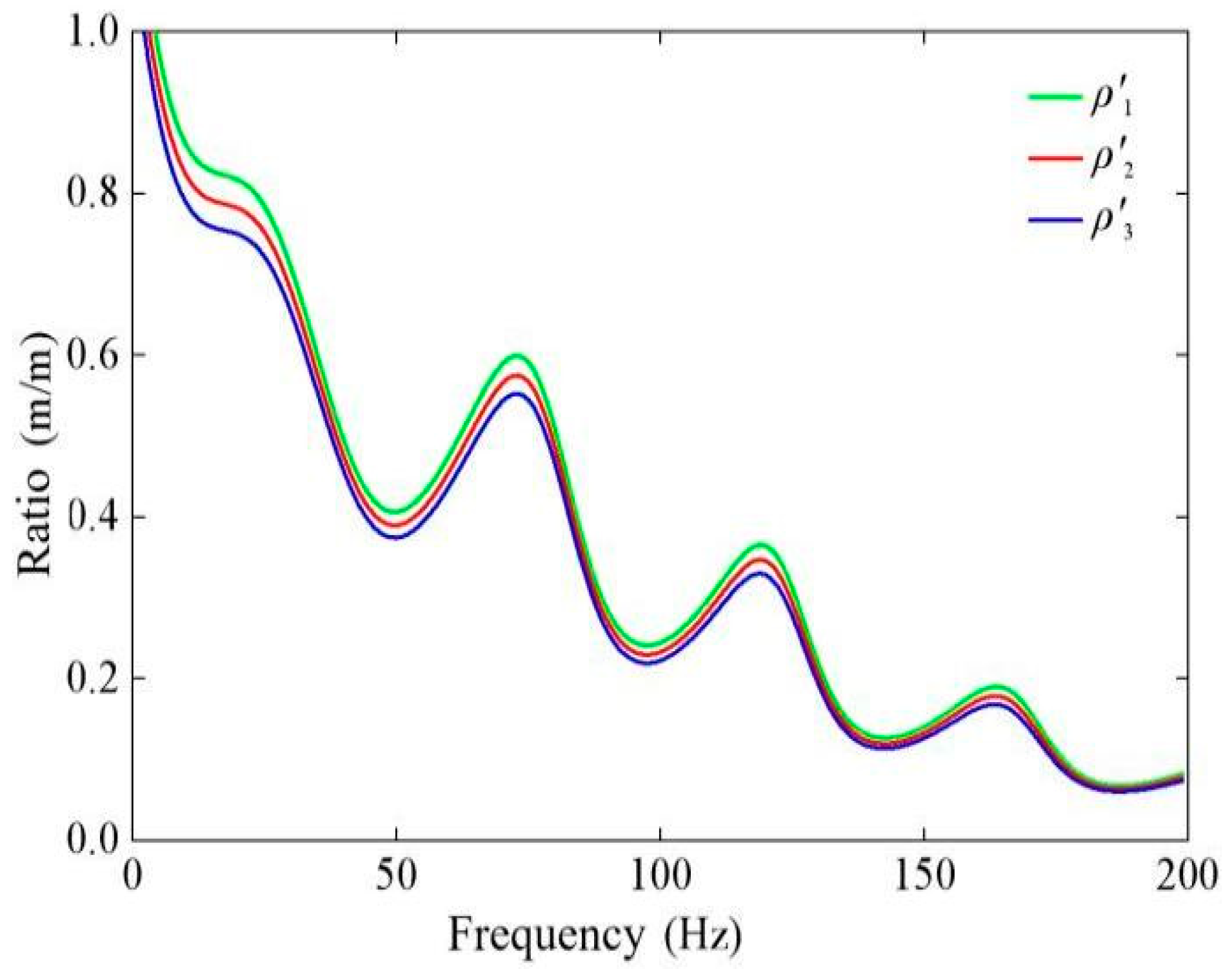
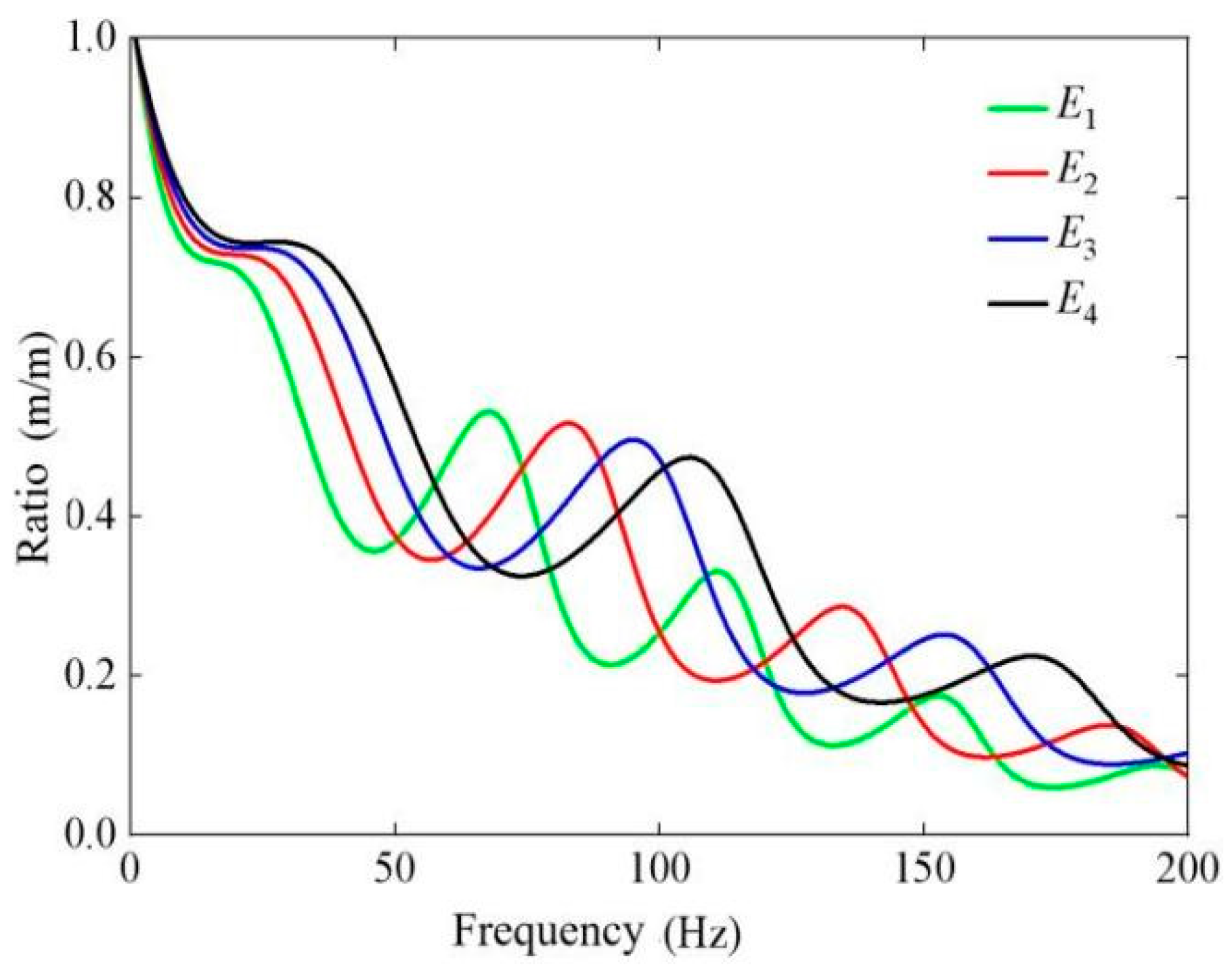
3.3.3. Effect of Elastic Modulus of Building Foundation

Under three different working conditions, where the elastic modulus of the building foundation is selected as E′₁ = 28.0 GPa, E′₂ = 30.0 GPa, and E′₃ = 32.5 GPa, with the other parameters unchanged, the calculation equation for the coupling loss coefficient is applied. The resulting variations in the coupling loss coefficient of the soil–structure transfer function with different building foundation elastic moduli are illustrated in Figure 16. This analysis provides insights into how changes in the elastic modulus of the building foundation affect the coupling loss coefficient and, consequently, the soil–structure interaction dynamics.

When the elastic modulus of the building foundation (E’) changes from 28.0 GPa to 32.5 GPa, the coupling loss coefficient gradually decreases in the frequency band from 10 to 30 Hz. This suggests that the displacement ratio between the building foundation and the free field soil mass decreases gradually within this specific frequency range. However, there is no significant effect on the coupling loss coefficient when there are changes in the elastic modulus of the building foundation in other frequency bands. This observation indicates that the impact of the elastic modulus on the coupling loss coefficient is frequency-dependent and more pronounced within the specified frequency range.

3.4. Effect of Soil Parameter Variation on Coupling Loss Coefficient

3.4.1. Effect of Soil Mass Elastic Modulus E on Coupling Loss Coefficient

To explore the impact of changes in the elastic modulus of the soil mass on the coupling loss coefficient in the soil-–structure transfer function, different values for the soil elastic modulus (E) were considered: E₁ = 100 MPa, E₂ = 150 MPa, E₃ = 200 MPa, and E₄ = 250 MPa. By utilizing the expression of the coupling loss coefficient introduced in Section 2.2, the resulting variations in the coupling loss coefficient of the soil–structure transfer function with different soil mass elastic moduli are illustrated in Figure 17. This analysis sheds light on how alterations in the soil elastic modulus influence the coupling loss coefficient and, consequently, the soil–structure interaction dynamics.

From Figure 17, it is apparent that as the soil elastic modulus (E) changes from 100 MPa to 250 MPa, the coupling loss coefficient gradually increases. This implies that the displacement ratio between the building foundation and the soil in the free field increases gradually. With the increase in the soil elastic modulus (E), the stiffness of the soil mass becomes larger, resulting in a smaller stiffness ratio between the soil and the building foundation. Consequently, the interaction between the soil mass and the building foundation becomes less pronounced, leading to an increase in the coupling loss coefficient.

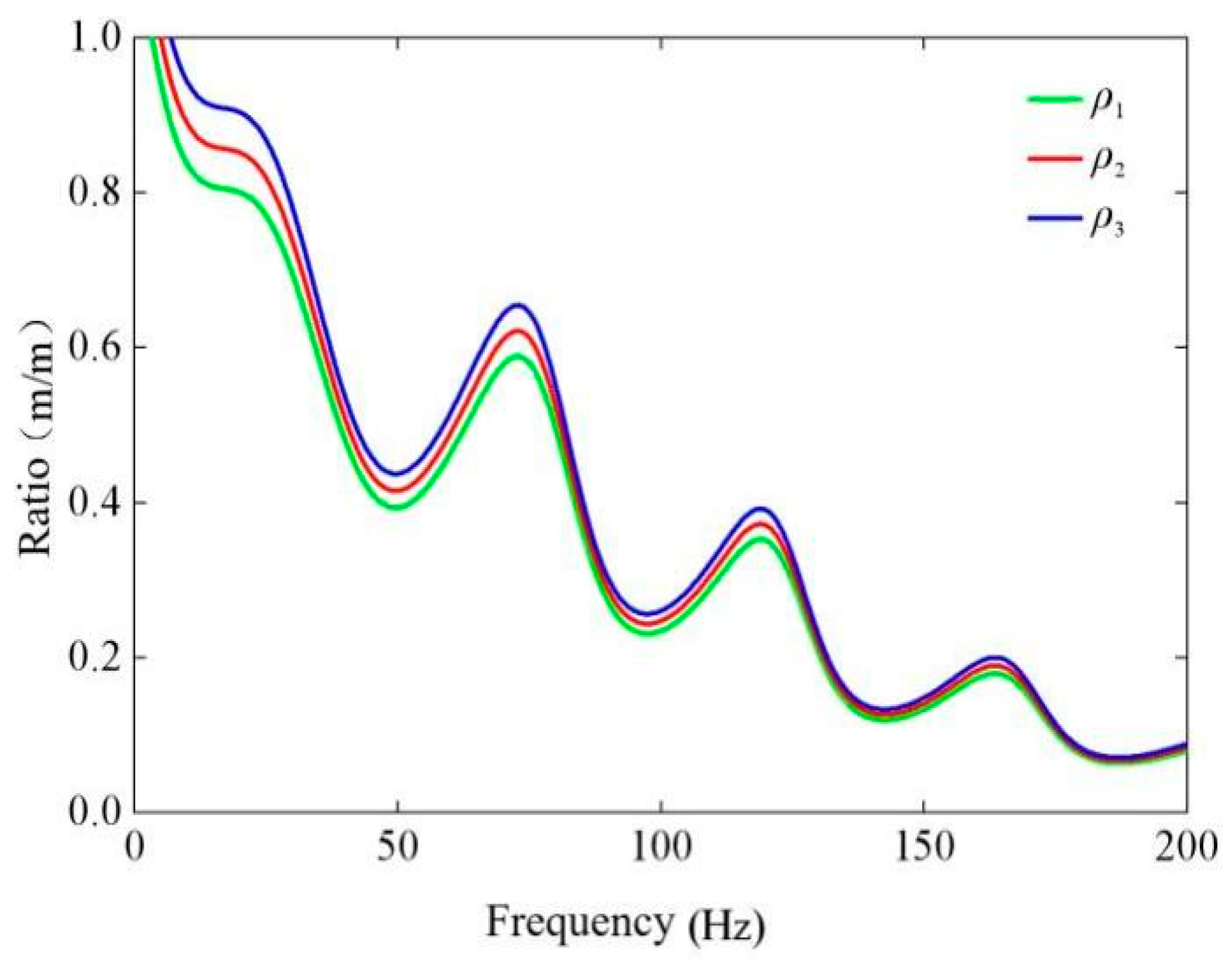
3.4.2. Effect of Soil Mass Density on Coupling Loss Coefficient

For three different working conditions, where the soil density is selected as ρ₁ = 1900 kg/m³, ρ₂ = 2000 kg/m³, and ρ₃ = 2100 kg/m³, with the other parameters unchanged, the calculation equation for the coupling loss coefficient is applied. The resulting variations in the coupling loss coefficient of the soil–structure transfer function with different soil mass densities are illustrated in Figure 18. This analysis provides insights into how changes in the soil density affect the coupling loss coefficient and, consequently, the soil–structure interaction dynamics.

From Figure 18, it is evident that as the density ρ of the soil mass changes from 1900 kg/m³ to 2100 kg/m³, the coupling loss coefficient gradually increases. This indicates a gradual increase in the displacement ratio between the building foundation and the free field soil mass. The increase in the coupling loss coefficient is attributed to the increasing density of the soil mass. As the soil density increases, the contact area between the soil particles per unit volume also increases, enhancing the overall stiffness of the soil mass. This, in turn, results in a gradual increase in the stiffness ratio between the soil and the concrete foundation, making the interaction between the soil mass and the concrete foundation less pronounced.

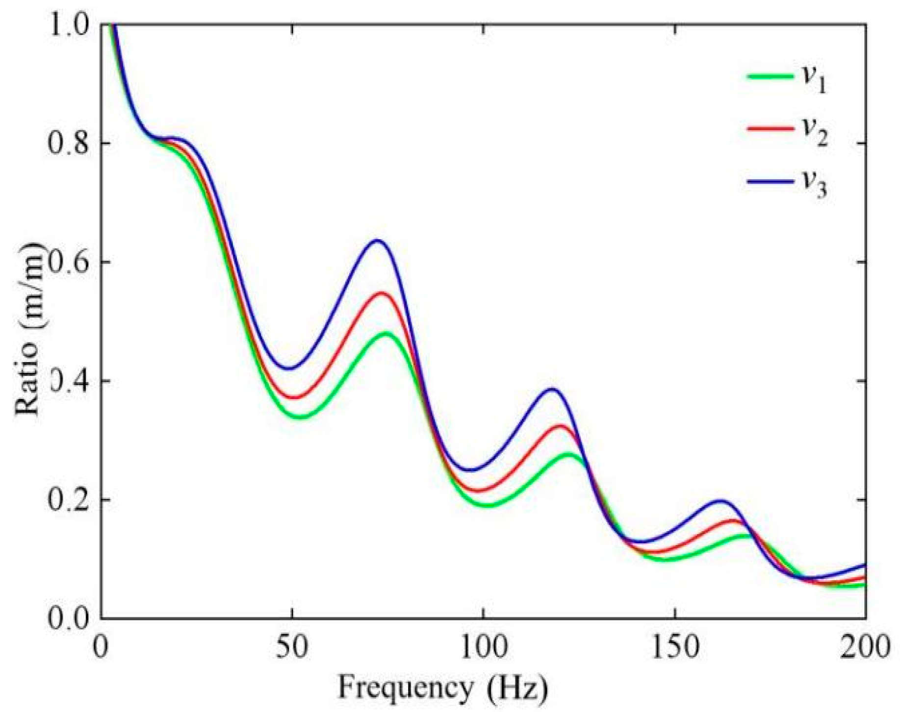
3.4.3. Effect of Soil Poisson’s Ratio on Coupling Loss Coefficient

For three different working conditions, where the Poisson’s ratio of the soil is selected as ν₁ = 0.2, ν₂ = 0.3, and ν₃ = 0.4, with the other parameters unchanged, the calculation equation for the coupling loss coefficient is applied. The resulting variations in the coupling loss coefficient of the soil–structure transfer function with different Poisson’s ratios of the soil mass are illustrated in Figure 19. This analysis provides insights into how changes in the Poisson’s ratio of the soil affect the coupling loss coefficient and, consequently, the soil–structure interaction dynamics.

From Figure 19, it is apparent that as the Poisson’s ratio (ν) of the soil mass changes from 0.2 to 0.4, the coupling loss coefficient in the soil–structure transfer function increases gradually. This implies a gradual increase in the displacement ratio between the building foundation and the soil mass. Moreover, the interaction force between the soil mass and the building foundation decreases gradually. The observed trends suggest that changes in the Poisson’s ratio of the soil affect the soil–structure interaction dynamics, influencing the coupling loss coefficient accordingly.

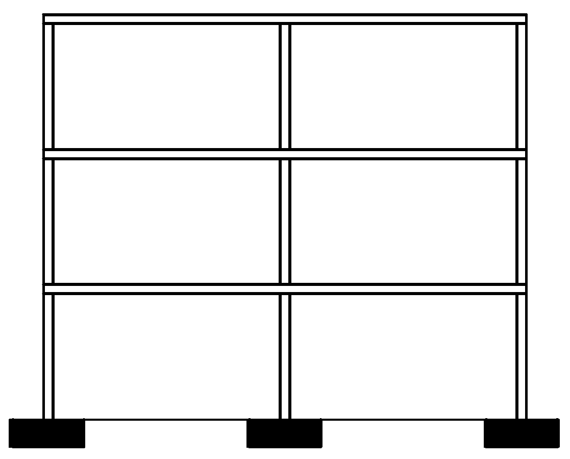
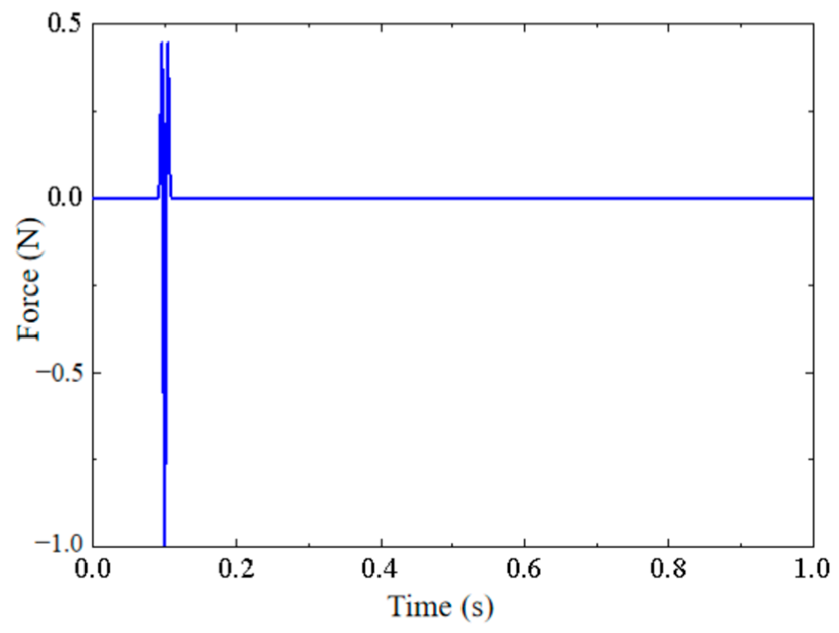
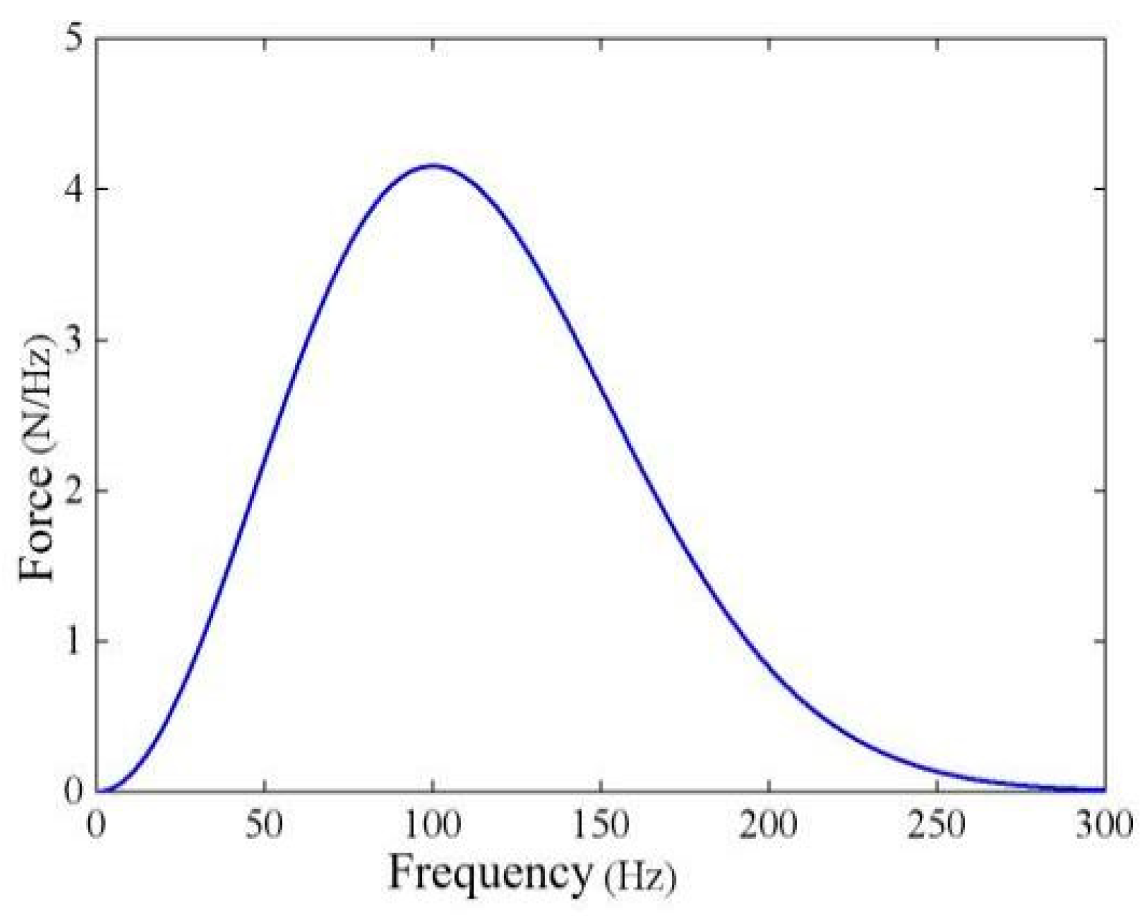
4. Case Study: Building Foundation Response under Ricker Pulse

The vertical displacement expression of the building foundation is:

$$U_0^{foot}(f)=U_0^{soil}(f)\cdot C_l(f)$$

(37)

The expression for the coupling loss coefficient C_l(f) has been derived in Section 2.2. Consequently, the vertical free field displacement of the building foundation under the action of a Ricker pulse can be denoted as U₀^soil (as shown in Figure 20). The vertical displacement U₀^foot of the building foundation under the action of a Ricker pulse can then be determined using this expression.

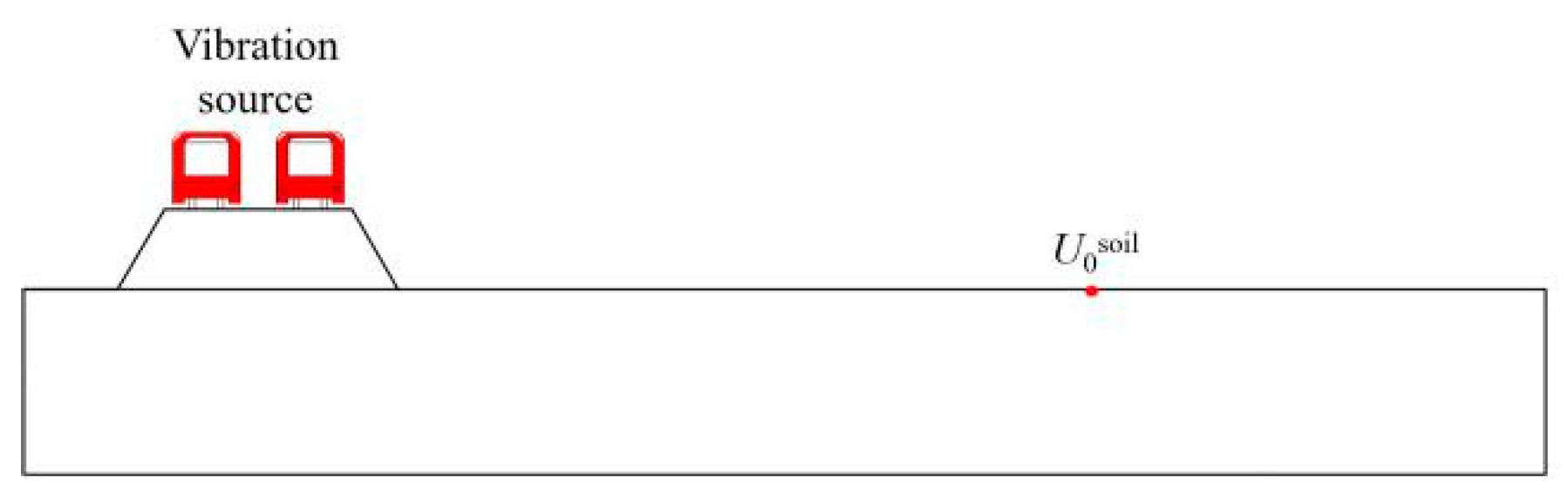
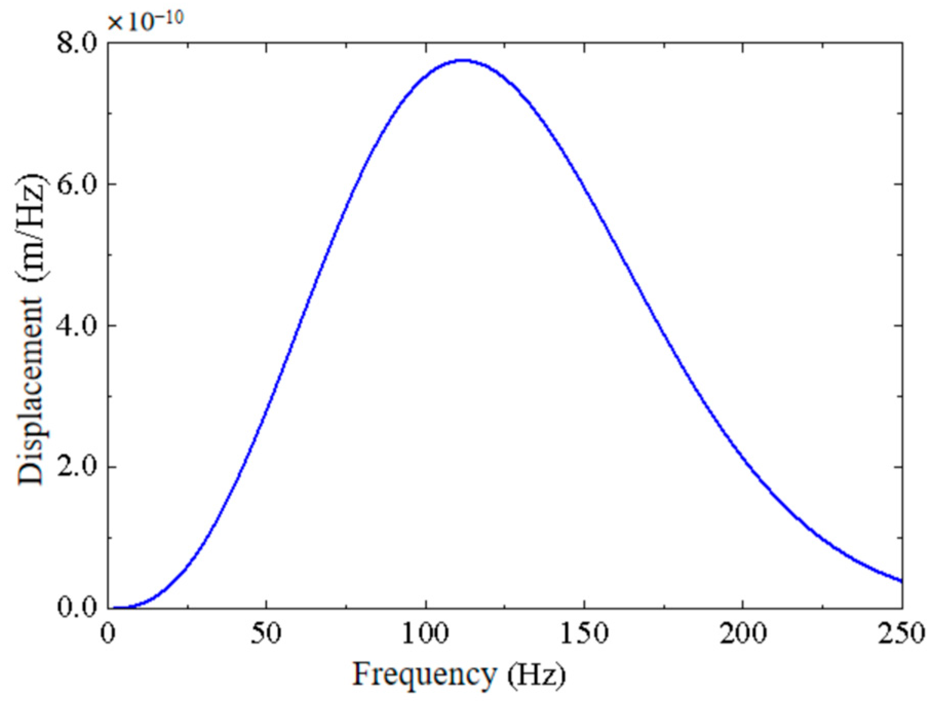
4.1. Solution of Vertical Displacement Response of Free Field under Ricker Pulse

In Equation (38), the expression for the vertical displacement of the free field particle at the building foundation under a simple harmonic load F(t) = Pe^iωt is as follows:

$$U_0^{soil}=\frac{p}{\mu }\overline{\xi }\sqrt{\frac{1}{r{\lambda }_r}}\cos \left(\omega t-k_{r}r-\frac{\pi }{4}\right)$$

(38)

The data of the case in Section 3.1 are input into the above equation, and the free field displacement U₀^soil curve at S₃ of the building foundation under a Ricker pulse is obtained as follows.

From Figure 21, it can be observed that the frequency corresponding to the peak vertical displacement is approximately 120 Hz. This aligns with the peak of the Ricker pulse excitation frequency spectrum curve.

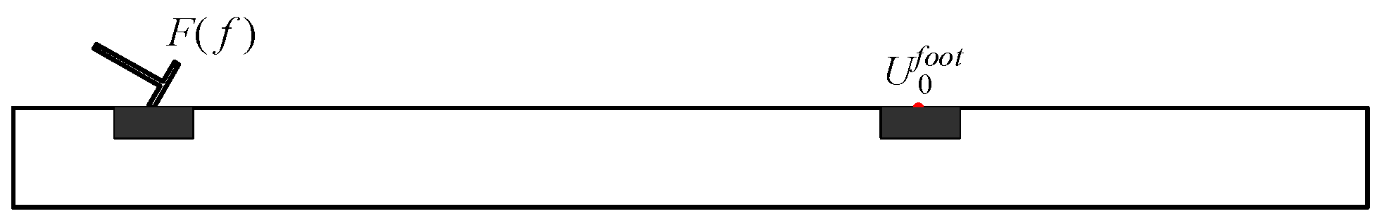
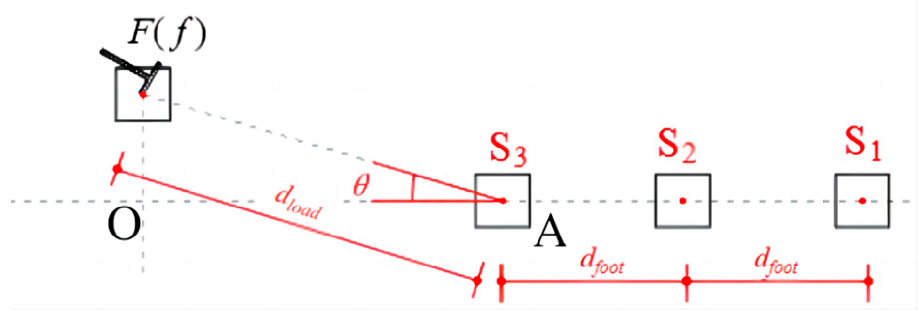
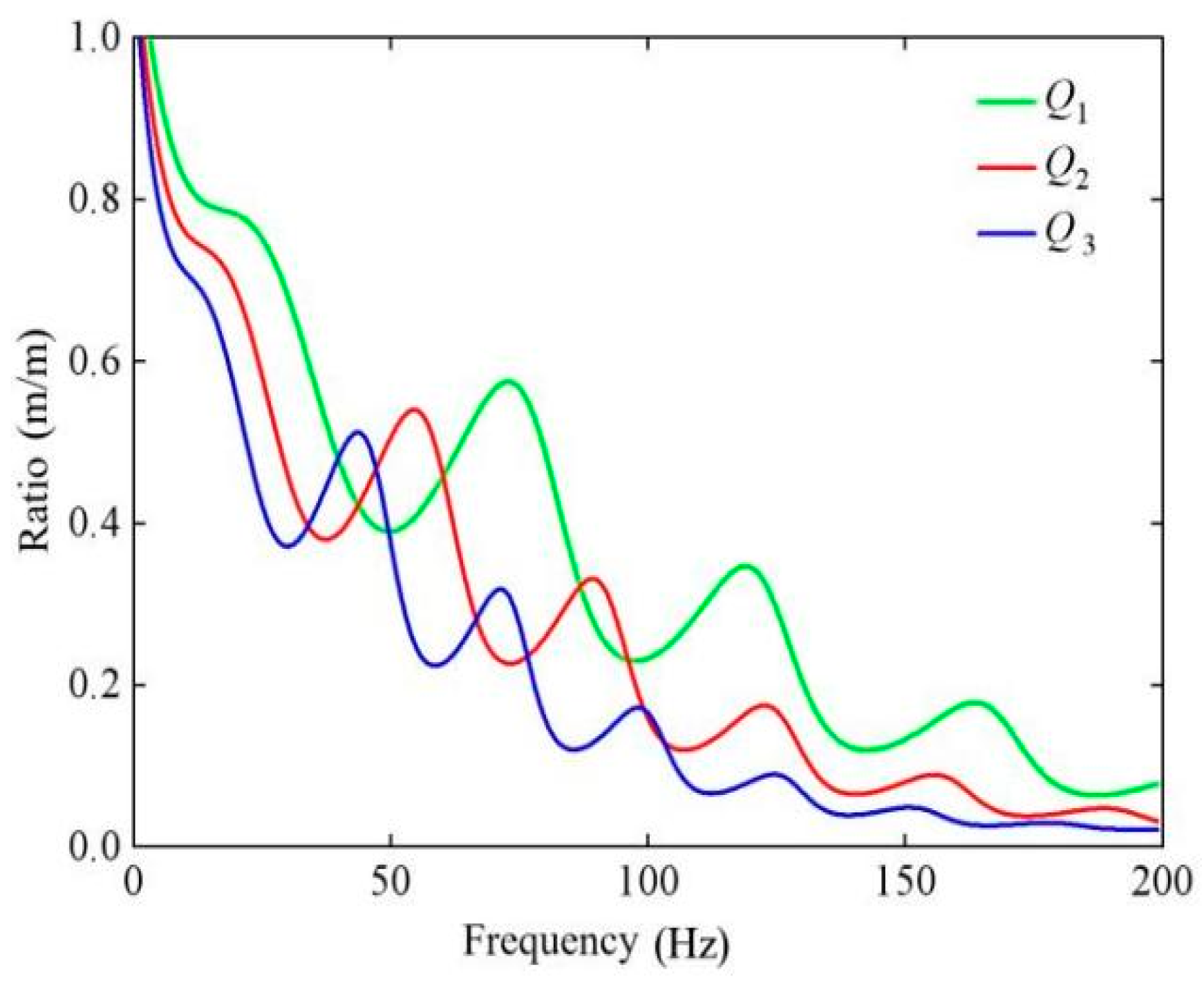
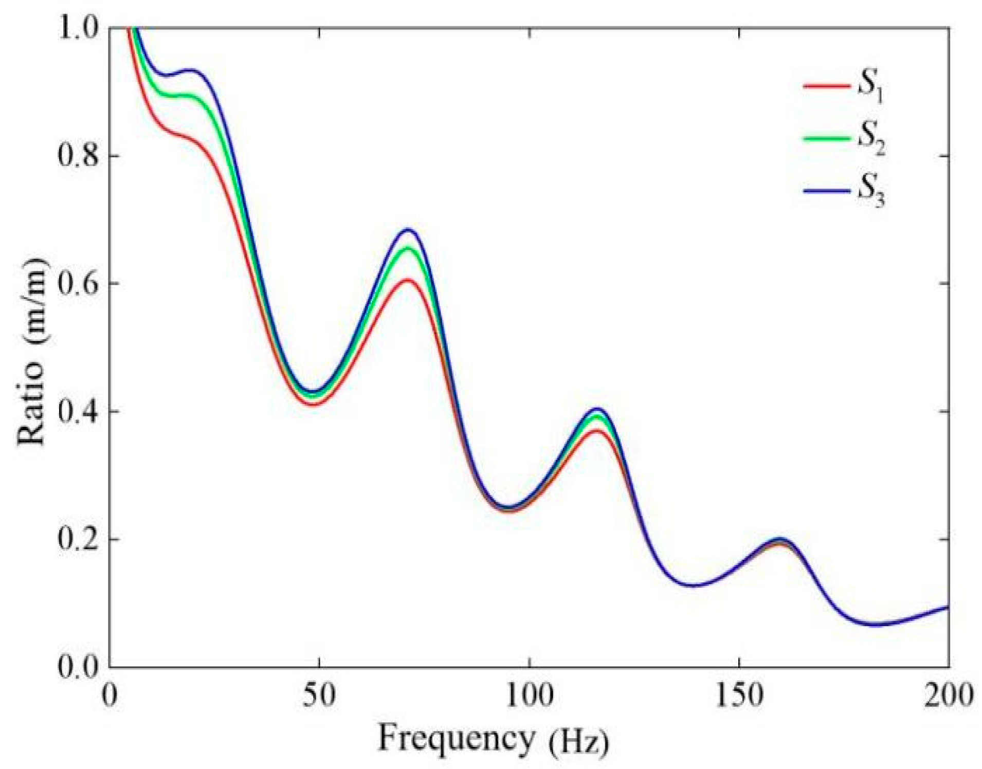
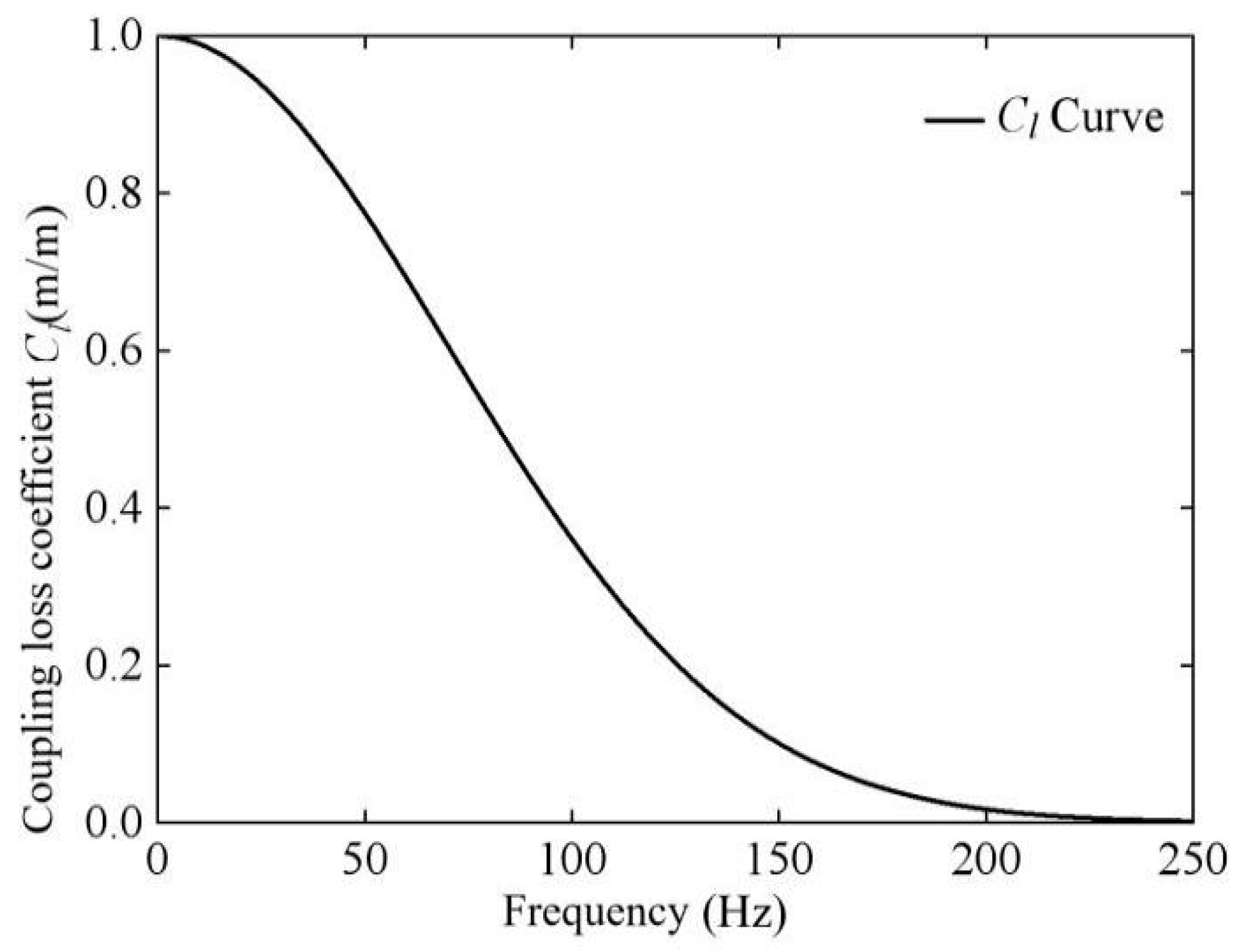
4.2. Solution for the Coupling Loss Coefficient of Building Foundation

According to the expression C_l of the coupling loss coefficient in Section 2.2, the coupling loss coefficient curves of S₁, S₂, S₃ of the building foundation can be drawn in Figure 22.

Recognizing the proximity of the coupling loss coefficient curves for different foundations, a Gaussian curve is contemplated for fitting to derive the coupling loss coefficient for the entire building. The expression is:

$$G\left({\gamma }_R\right)={\exp }^{-\frac{{({\gamma }_R)}^2}{2c^2}},{\gamma }_R=\frac{\omega B_f}{4\pi C_s}$$

(39)

The variable c serves as a real constant, representing the standard deviation. The determination of the standard deviation c value is achieved through fitting the coupling loss coefficient curves of the building foundations S₁, S₂, and S₃ using the Isqnonlin function in MATLAB. The resulting coupling loss coefficient curves, denoted as C_l, fitted to the building foundations S₁, S₂, and S₃, are depicted in Figure 23.

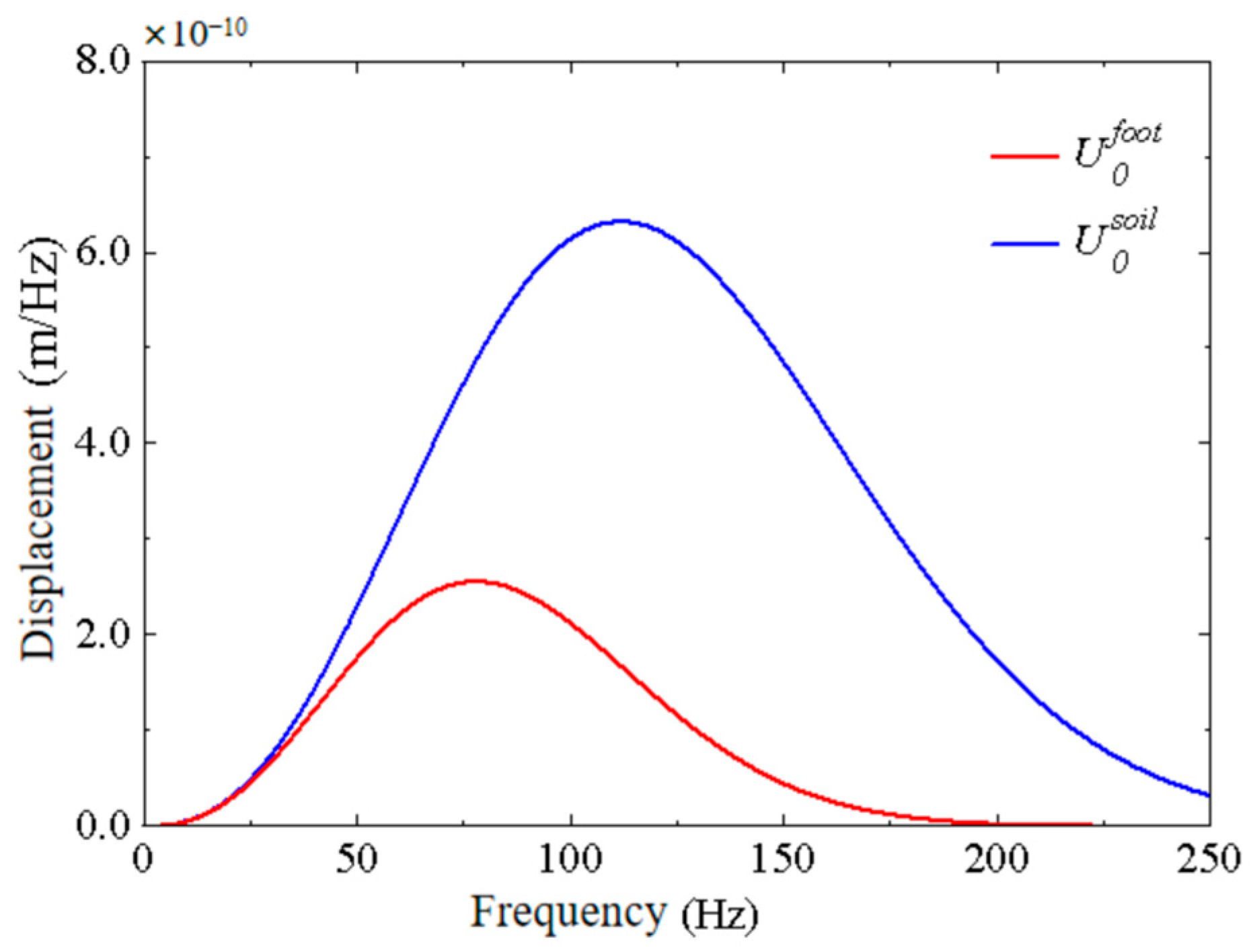
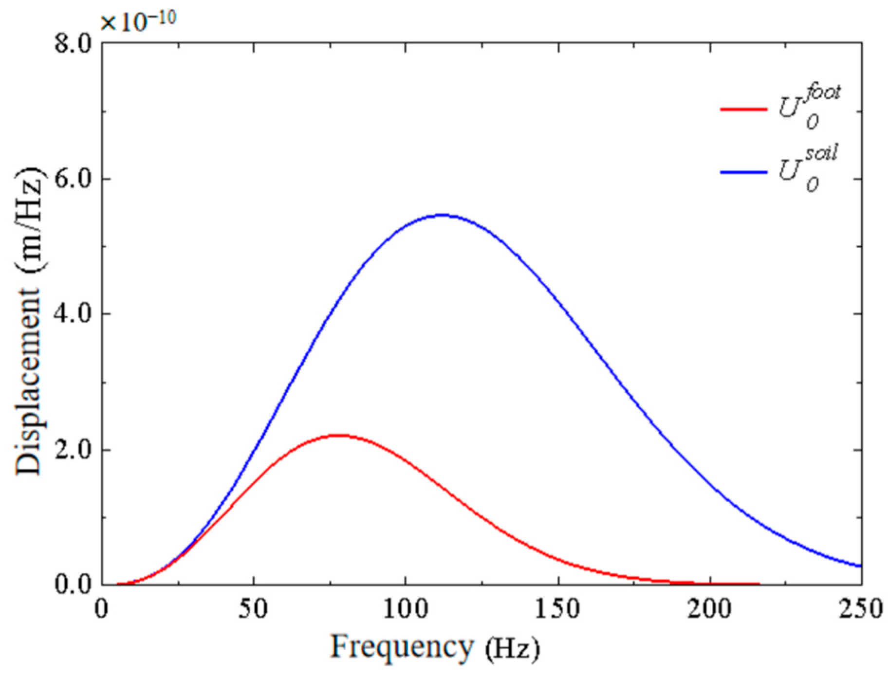
4.3. Solution of Vertical Displacement of Building Foundation

Considering that the vibration response of the building foundation is given by U₀^foot(f) = U₀^soil(f)⋅C_l(f), the vertical displacement curve of the free field at the building foundation S3 under Ricker pulse action (Figure 21) is multiplied by the fitting coupling loss coefficient, as illustrated in Figure 24. Consequently, the vertical displacement values U₀^foot(f) of the building foundation S₃ under a Ricker pulse are obtained, as depicted in Figure 25.

Likewise, the vertical displacement values U₀^foot(f) and free field displacement values U₀^soil(f) of the building foundation S₂ under a Ricker pulse are illustrated in Figure 26.

It is evident from the figure that the frequency corresponding to the peak vibration response of the building foundation is higher than that corresponding to the peak vibration response of the soil mass. This discrepancy can be attributed to the significant differences in the elastic modulus and density between the concrete foundation and the soil mass. Accounting for the coupling loss coefficient helps mitigate the response of the high-frequency vibration component. The vertical displacement value U₀^foot(f) and free field displacement value U₀^soil(f) of the building foundation Sb under a Ricker pulse are presented in Figure 27.

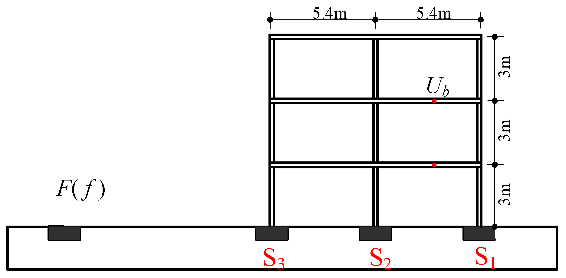
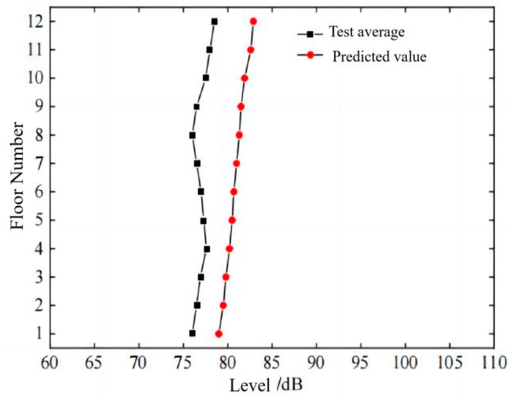
5. Application Case: Prediction of High-Speed Train-Induced Soil–Structure Vibration

To validate the accuracy of the soil–structure transfer function method in predicting the vibrations induced by high-speed trains on a proposed building, a comparison was performed with actual measurement data. The experimental building is a 12-story reinforced concrete structure with a total height of 36.6 m above ground. The first floor has a height of 3.6 m, while the remaining floors are each 3 m high. The total length is 45 m, comprising 10 rooms, with each bay measuring 4.5 m. The spans are 6 m + 2.4 m + 6 m. The distance between the centerline of the railway track and the building is 12 m, as illustrated in Figure 28. The soil parameters of the experimental site are shown in

Table 1. Soil parameters at the test site.

Type	Elastic Modulus E/MPa	Poisson	Density (kg/m3)	Thickness (m)
Backfill	29	0.4	1700	1
Sand clay	127	0.33	1880	3
Coarse sand	150	0.33	1918	4
Gravel sand	430	0.29	1211	40

.

The measured values of the maximum vertical vibration acceleration are selected for the analysis. The soil and building parameters at the test site are then substituted into the soil–structure transfer function to calculate the building’s vibration response. The vibration response of each floor is analyzed using the vibration acceleration level (VAL) as an indicator.

The measured values are to be compared with the calculated results from the analytical coupling loss coefficient, as illustrated in Figure 29. It can be observed that the test values of the building vibrations generally show an increasing trend with the number of floors, although it is not consistently monotonic. The results obtained using the soil–structure transfer function method exhibit a monotonic increase and slightly surpass the measured average value. Both numerical trends demonstrate an overall increase with the number of floors, and the values are relatively close, indicating the feasibility of the soil–structure transfer function method in predicting the vibrational response of buildings induced by train activity.

6. Conclusions

This paper successfully derives the calculation equation for the transfer function coupling loss coefficient and thoroughly analyzes the factors influencing the coupling loss coefficient, such as the angle, soil mass parameters, and building foundation parameters. Furthermore, the obtained vertical displacement values of the building foundation under a Ricker pulse are compared with references, providing a solid foundation for calculating the building’s vibration response.

(1) Advantages of the Coupling Loss Coefficient in the Soil–Structure Transfer Function:

The coupling loss coefficient streamlines the calculation process, eliminating the need for testing and extensive modeling. Theoretical analysis allows for a quick and accurate determination of the displacement transfer relationship between the soil and the building, effectively illustrating their interaction.

(2) Complexity and Parameter Dependencies of the Coupling Loss Coefficient:

The coupling loss coefficient exhibits complexity and dependencies on the building foundation and soil mass parameters. The analysis reveals that increasing the building foundation size results in an increased coupling loss coefficient, indicating a reduction in the displacement ratio between the building foundation and the free field soil mass, leading to decreased interaction force. Moreover, the coupling loss coefficient is influenced by changes in the elastic modulus, density, and Poisson’s ratio of the building foundation and soil mass.

(3) Insights from the Coupling Loss Coefficient Curve:

The coupling loss coefficient curve demonstrates values ranging from 0 to 1, signifying that in the presence of a building foundation, Rayleigh wave transmission and reflection occur, mitigating the vibration induced by incident Rayleigh waves.

In summary, the findings of this study offer valuable insights into the coupling loss coefficient, its dependencies, and its role in reducing the vibrations induced by Rayleigh waves. Utilizing the soil–structure transfer function, this research efficiently forecasts the building vibrations induced by train activities. This method, after determining the coupling loss and floor amplification coefficients, integrates with a broad range of free field vibration data. It simplifies and enhances the predictions for structures influenced by various factors, such as construction, seismic events, road traffic, and explosions. By providing a versatile tool, the approach aids in swiftly and accurately anticipating vibrations, especially for prospective buildings near high-speed rail tracks.

References

- Krylov, V.V. On the Theory of Railway-Induced Ground Vibrations. J. De Phys. IV 1994, 4, 769–772. [Google Scholar] [CrossRef]
- Krylov, V.V. Generation of Ground Vibrations by Superfast Trains. Appl. Acoust. 1995, 44, 149–164. [Google Scholar] [CrossRef]
- Krylov, V.V. Effects of Track Properties on Ground Vibrations Generated by High-Speed Trains. Acust.-Acta Acust. 1998, 84, 78–90. [Google Scholar]
- Kurzweil, L.; Cobb, W.; Dinning, M. Urban Rail Noise Abatement Program: A Description; Urban Mass Transportation Administration: Washington, DC, USA, 1980. [Google Scholar]
- Hirokazu, T.; Taro, U.; Satoshi, F. Component modal synthesis method for 3D seismic response analysis of subground-foundation-superstructure systems. World Earthq. Eng. 1988, 4, 43–47. [Google Scholar]
- Yue, J. Measurement and Numerical Simulation Analysis of building vibration caused by subway traffic. J. Petrol. Geophys. 2020, 41, 2756–2764. [Google Scholar]
- Lei, F. Research on Prediction Method of Environmental Vibration Caused by High-Speed Train Based on Random Forest Algorithm; Beijing Jiaotong University: Beijing, China, 2020. [Google Scholar]
- Colaço, A.; Costa, P.A.; Amado-Mendes, P.; Calçada, R. Vibrations induced by railway traffic in buildings: Experimental validation of a sub-structuring methodology based on 2.5D FEM-MFS and 3D FEM. Eng. Struct. 2021, 240, 112381. [Google Scholar] [CrossRef]
- Colaço, A.; Costa, P.A.; Castanheira-Pinto, A.; Amado-Mendes, P.; Calçada, R. Experimental Validation of a simplified soil-structure interaction approach for the prediction of vibrations in buildings due to railway traffic. Soil Dyn. Earthq. Eng. 2021, 141, 106499. [Google Scholar] [CrossRef]
- Colaço, A.; Barbosa, D.; Costa, P.A. Hybrid soil-structure interaction approach for the assessment of vibrations in buildings due to railway traffic. Transp. Geotech. 2022, 32, 100691. [Google Scholar] [CrossRef]
- Sadeghi, J.; Vasheghani, M. Safety of buildings against train induced structure borne noise. Build. Environ. 2021, 197, 107784. [Google Scholar] [CrossRef]
- Farahani, M.V.; Sadeghi, J.; Jahromi, S.G.; Sahebi, M.M. Modal based method to predict subway train-induced vibration in buildings. Structures 2023, 47, 557–572. [Google Scholar] [CrossRef]
- Sadeghi, J.; Vasheghani, M. Improvement of current codes in design of concrete frame buildings: Incorporating train-induced structure borne noise. J. Build. Eng. 2022, 58, 104955. [Google Scholar] [CrossRef]
- Ibrahim, Y.E.; Nabil, M. Finite element analysis of multistory structures subjected to train induced vibrations considering soil-structure in-teraction. Case Stud. Constr. Mater. 2021, 15, 100592. [Google Scholar]
- ISO 14837-1; Mechanical Vibration–Groundborne Noise and Vibration Arising from Rail Systems—Part 1: General Guidance. International Organization for Standardization: Geneva, Switzerland, 2005.
- Richart, F.E., Jr.; Hall, J.R., Jr.; Woods, R.D. Vibration of Soil and Foundation; Prentice-Hall: Saddle River, NJ, USA, 1970. [Google Scholar]
- Zhao, R. Theoretical Research and Numerical Analysis of Effects of Filling Ditch on Environmental Vibration Caused by Running Trains; Beijing Jiaotong University: Beijing, China, 2017. [Google Scholar]
- Du, X.-L. Theories and Methods of Wave Motion for Engineering; Science Press: Beijing, China, 2009. (In Chinese) [Google Scholar]
- Maurice, J.Y. The reflection and transmission of Rayleigh waves. Univ. Appl. Phys. 2012, 112, 103520. [Google Scholar]
- Lapwood, E.R. The Transmission of a Rayleigh Pulse round a corner. Geophys. J. R. Astron. Soc. 1961, 4, 174–196. [Google Scholar] [CrossRef]
- Asadi Jafari, M.H.; Zarastvand, M.; Zhou, J. Doubly curved truss core composite shell system for broadband diffuse acoustic insulation. J. Vib. Control 2023. [Google Scholar] [CrossRef]
- Qiu, Y.; Zou, C.; Hu, J.; Chen, J. Prediction and mitigation of building vibrations caused by train operations on concrete floors. Appl. Acoust. 2024, 219, 109941. [Google Scholar] [CrossRef]
- Hu, J.; Zou, C.; Liu, Q.; Li, X.; Tao, Z. Floor vibration predictions based on train-track-building coupling model. J. Build. Eng. 2024, 89, 109340. [Google Scholar] [CrossRef]
- He, L.; Tao, Z. Building Vibration Measurement and Prediction during Train Operations. Buildings 2024, 14, 142. [Google Scholar] [CrossRef]
- Ma, M.; Xu, L.H.; Liu, W.F.; Tan, X. Semi-analytical solution of a coupled tunnel-soil periodic model with a track slab under a moving train load. Appl. Math. Model. 2024, 128, 588–608. [Google Scholar] [CrossRef]
- Bucinskas, P.; Andersen, L.V. Semi-analytical approach to modelling the dynamic behaviour of soil excited by embedded foundations. Procedia Eng. 2017, 199, 2621–2626. [Google Scholar] [CrossRef]
- Bucinskas, P.; Andersen, L.V. Dynamic response of vehicle–bridge–soil system using lumped parameter models for structure–soil interaction. Comput. Struct. 2020, 238, 106270. [Google Scholar] [CrossRef]
- Persson, P.; Andersen, L.; Persson, K.; Bucinskas, P. Effect of structural design on traffic-induced building vibrations. Procedia Eng. 2017, 199, 2711–2716. [Google Scholar] [CrossRef]
- Bucinskas, P.; Ntotsios, E.; Thompson, D.J.; Andersen, L.V. Modelling train-induced vibration of structures using a mixed-frame-of-reference approach. J. Sound Vib. 2021, 491, 115575. [Google Scholar] [CrossRef]
- Bucinskas, P.; Persson, K. Numerical modelling of ground vibration caused by elevated high-speed railway lines considering structure-soil-structure interaction. Inst. Noise Control Eng. 2016, 253, 7017–7028. [Google Scholar]