Probabilistic Analysis of Strength in Retrofitted X-Joints under Tensile Loading and Fire Conditions

Abstract

In the present study, a total of 360 FE analyses were carried out on tubular X-joints strengthened with collar plates under brace tension under laboratory testing conditions (20 °C) and various fire conditions. The generated FE models were validated based on 31 tests. The FE analyses produced a comprehensive dataset that encapsulated resistance metrics, with detailed simulations of welds, contacts, and the incorporation of non-linear geometrical and material attributes. Twelve theoretical probability density functions (PDFs) were matched to the constructed histograms, with the maximum likelihood (ML) technique utilized to assess the parameters of these fitted PDFs. The theoretical PDFs, rigorously evaluated against the Anderson–Darling, Kolmogorov–Smirnov, and Chi-squared tests, identified the Generalized Petrov distribution as the optimal model for capturing the resistance behaviors of X-joints under tensile load and varying fire conditions. The findings have led to the proposition of five detailed theoretical PDFs and cumulative distribution functions (CDFs), introducing a novel perspective for assessing and reinforcing the structural resilience of strengthened CHS X-joints in engineering practices.

1. Introduction

In offshore circular hollow section (CHS) structures, like jacket-type platforms, fire represents a critical design scenario due to the degradation of steel’s mechanical properties with increasing temperature. Understanding the behavior of CHS structures under high temperatures is crucial. Typically, CHS members are used as the primary elements in these structures, interconnected to create a CHS joint, and ensuring the overall integrity and performance of the structure in challenging conditions [1,2].

Static and dynamic deterministic analyses often result in conservative designs due to their reliance on limiting assumptions about the input parameters, many of which exhibit significant variability. This underscores the importance of reliability-based analysis and design methods, which treat key parameters as random variables.

Tubular nodes are pivotal to the structural integrity of jacket-type platforms, with failures frequently occurring at these critical nodes. Therefore, evaluating the reliability of such structures requires considering the potential failures of connections under diverse loading conditions.

Reliability analysis serves as a crucial technique for determining the likelihood of simultaneous failures by examining if the limit state function has been surpassed. The limit state function, defined as g = S − L, is integral to this evaluation. In this context, S signifies the nod’s capacity, and L represents the forces acting on the braces. A negative g value indicates a failure of the node under the given loading conditions. In structural reliability assessments, both the capacity S and the forces L acting on the braces are generally considered stochastic variables, each described by their PDFs. These PDFs encapsulate the inherent uncertainties associated with the variables. The PDF of the capacity illustrates the probability of the node enduring specific load levels, offering insights into its robustness. Similarly, the PDF of the forces in the braces outlines the likelihoods of various force levels encountered by the braces. X-connections are commonly used in jacket-type platforms, requiring rigorous design strategies to improve their structural reliability. Nonetheless, there is a notable absence of a PDF specifically characterizing the ultimate capacity of the stiffened X-connections. This study aimed to develop the PDF for the capacity of X-connections with collar plates under both laboratory testing conditions (20 °C) and elevated temperatures. Establishing this PDF will enable engineers to make well-informed decisions about the safety and reliability of these essential structural components.

To date, various strategies have been developed to bolster the static resistance of CHS joints under both standard and elevated temperature conditions. While many reinforcing techniques, including the use of doubler plates, racks/ribs, and internal rings, are designed to be integrated into the construction phase of structures, only a select few methods, such as the application of collar plates and outer rings, provide the versatility for deployment and sustained effectiveness throughout the design and ongoing operational phases of a structure. These methods present effective solutions for the reinforcement and repair of joints within both existing and newly constructed frameworks. The process of reinforcing a CHS joint involves affixing plates externally to the chord (primary) component, thereby creating what is known as a collar plate-reinforced joint (refer to Figure 1). In Figure 1, the parameter β, which is the ratio of the brace diameter to the chord diameter, increases the brace diameter when the chord diameter is held constant. The parameter γ, defined as the ratio of the chord radius to its thickness, results in a thinner chord when γ increases while keeping the chord diameter constant. For the parameter τ, representing the ratio of brace thickness to chord thickness, an increase in τ leads to a thicker brace in models where the γ ratio remains unchanged. The parameter α is the ratio of the chord length to its radius. The parameter η, which measures the collar plate length relative to the brace diameter, results in a longer collar plate when η increases and the brace diameter is fixed. Finally, the parameter τ_c, which is the ratio of the collar plate thickness to chord thickness, leads to a thicker collar plate when τ_c increases in models with a constant γ value.

Nassiraei et al. [3] examined how the addition of retrofit plates influences both the peak load-bearing capacity and the patterns of failure in CHS X-joints when exposed to axial loading. They suggested a formula to predict the resistance of X-joints with the plate in compression. Additionally, some experimental tests were tested by Shao [4] to evaluate the role of the plate thickness and length on the load–displacement behavior of CHS T-joints. In addition, Choo et al. [5,6] and Van der Vegte [7] evaluated the resistance and failure modes of X-, T-, and Y-joints with the plate under axial and in-plane bending loads. They suggested some formulae for determining the resistance under laboratory testing conditions (20 °C). Gao et al. [8] determined the threshold temperature for connections equipped with a collar plate. Three unstrengthened CHS T-joints under compression and fire conditions were tested by Tan et al. [9]. They obtained the resistance of the joints at high temperatures. Ozyurt et al. [10] and Ozyurt and Wang [11] assessed how exposure to fire affects the load-bearing capacity of non-reinforced CHS joints under axial and bending forces. They suggested reduction factors for determining the ultimate resistance. Azari-Dodaran and Ahmadi [12] numerically explored TT-joints under fire conditions. Additionally, they suggested some formulae to calculate the resistance. Pandey and Young [13] evaluated the static behavior of high-strength X-joints following exposure to fire. Nassiraei [14] explored the best probabilistic model for the resistance of the strengthened T-/Y-joints under a compressive load. Zhao et al. [15] explored the random distribution of the resistance in a corrosion environment. Also, the cold-formed elliptical and cold-formed semi-oval sections in hollow steel section joints are studied in Refs. [16,17,18,19,20,21,22]. The use of 3D printing technology and structural optimization [23,24,25,26] on tubular nodes is a good way to improve the performance of the joint.

According to the findings presented, there is an absence of research on how joints, when fitted with collars, behave in terms of resistance probability distributions under laboratory testing conditions (20 °C) and fire conditions. On the contrary, this retrofitting choice can remarkably improve the performance of joints at the time of both design and operation.

The investigation presents an analysis of the likelihood distributions for the load resistance of X-configured joints fitted with retrofit plates, subjected to tensile forces under normal and multiple fire conditions. To achieve this aim, the data produced from 360 FE models (FEMs) (Figure 1), confirmed via 31 tests, were applied. The attributes related to non-linear geometry and materials were established within the FEMs. The welding joints that attach the stiffener plates to the primary element were represented (indicated in blue in Figure 1). Additionally, a meticulous depiction was made of the engagement between the main structure’s exterior surfaces and the interior sides of the strengthening plates. The outcomes from finite element (FE) analyses were employed to recommend the probabilistic models for the maximum load capacity of X-joints strengthened with retrofitting plates under axial tension at various temperatures. Through a detailed parametric study, five robust datasets were generated. To identify the most accurate probabilistic distribution models for this application, twelve distinct distributions were applied to the data, with their efficacy assessed via Anderson–Darling, Chi-squared, and Kolmogorov–Smirnov tests for goodness-of-fit. Subsequently, to appraise the fit quality, the three tests were used for 60 cases (12 diverse PDFs for five samples). Finally, the best distributions were suggested and defined for the ultimate resistance in X-joints strengthened with the retrofitting plates at all temperatures.

2. Generation of the Databases

Using ANSYS version 19, 360 FEMs were created to develop databases detailing the resistance characteristics of retrofitted X-joints. This section outlines the methodology used in conducting the FE modeling and analysis of strengthened X-joints, with the ANSYS software version 19, serving as the platform for the simulations.

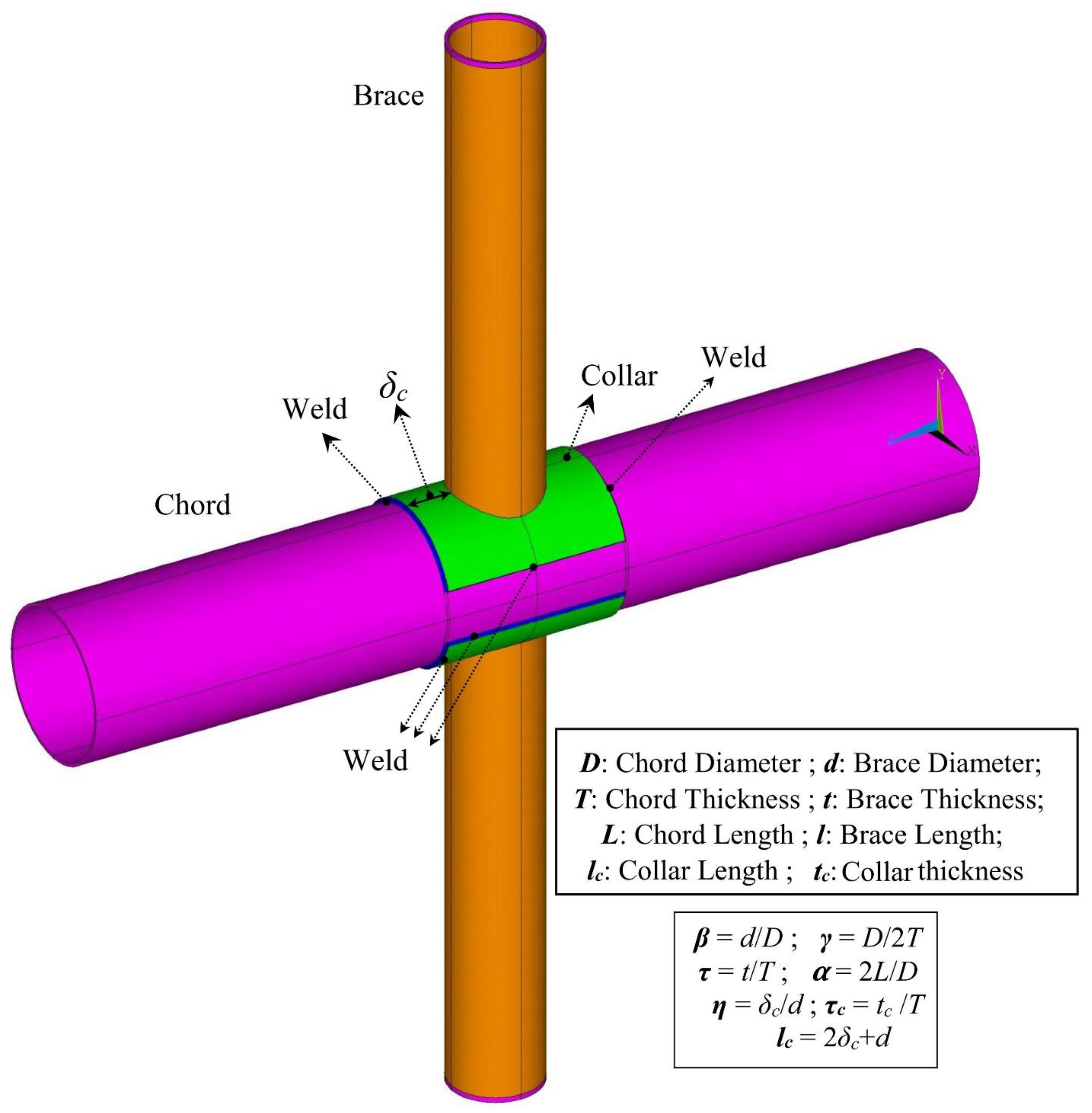
2.1. Finite Element (FE) Modeling

2.1.1. Weld Modeling

Fung et al. [27] examined how weld modeling affects the strength, discovering a nearly 10% difference in the strength between welded and non-welded joints. Meanwhile, Azari-Dodaran and Ahmadi [12] found that for tubular TT-joints at high temperatures, the strength discrepancy due to welds was under 5%, indicating that weld profile inclusion might be unnecessary. In contrast, this study incorporated welds in the FE model to achieve more precise results [28]. The American Welding Society (AWS) [29] provides specifications for welding tubular nodes, highlighted in blue in Figure 1. These guidelines dictate the end preparation, fit-up or root opening, the angle included in the joint, and the dimensions of the finished weld, all of which are dependent on the specific dihedral angle of the joint. Equation (1) specifies the weld’s horizontal dimension at critical points such as the crown and saddle, determined by the corresponding dihedral angle.

$$\psi (\mathrm{deg}.)=\left\{\begin{array}{c}Crown:\\ Saddle:\end{array}\right.\begin{array}{c}90\\ 180-{\cos }^{-1}\left(\beta \right)\hspace{0.17em}\end{array}\to W_h\hspace{0.17em}(mm)=0.5t\left[\frac{{135}^{\circ }-\psi (\mathrm{deg}.)}{{45}^{\circ }}\right]$$

(1)

2.1.2. Material Properties

The assessment made use of the von Mises yield criterion. The yield stress, Young’s module, and Poisson of the members are 330 MPa, 208 GPa, and 0.3. The material characteristics of the steel members (main, braces, retrofitting plates, and welds) under conditions of fire were specified as Equations (2)–(9) (EN 1993-1-2 [30]).

$$\mathrm{for} \epsilon \le {\epsilon }_{p,T\hspace{1em}\hspace{1em}\hspace{1em}\hspace{1em}}\sigma =\epsilon E_{a,T\hspace{1em}\hspace{1em}\hspace{1em}\hspace{1em}\hspace{1em}\hspace{1em}\hspace{1em}\hspace{1em}}\mathrm{Tan}\mathrm{mod}=E_{a,T\hspace{0.17em}\hspace{0.17em}}$$

(2)

$$\mathrm{for} {\epsilon }_{p,T\hspace{0.17em}\hspace{0.17em}}\le \epsilon \le {\epsilon }_{y,T\hspace{1em}\hspace{1em}\hspace{1em}}\hspace{0.17em}\sigma =f_{p,T}-c+(\raisebox{1ex}{$b$}\!\left/ \!\raisebox{-1ex}{$a$}\right.){[a^2-{({\epsilon }_{y,T\hspace{0.17em}\hspace{0.17em}}-\epsilon )}^2]}^{0.5}\hspace{0.17em}\hspace{0.17em}\hspace{1em}\hspace{1em}\mathrm{Tan}\mathrm{mod}=\hspace{0.17em}\frac{b({\epsilon }_{y,T\hspace{0.17em}\hspace{0.17em}}-\epsilon )}{a{[a^2-{({\epsilon }_{y,T\hspace{0.17em}\hspace{0.17em}}-\epsilon )}^2]}^{0.5}}$$

(3)

$$\mathrm{for} {\epsilon }_{y,T\hspace{0.17em}\hspace{0.17em}}\le \epsilon \le {\epsilon }_{t,T\hspace{1em}\hspace{1em}\hspace{1em}}\hspace{0.17em}\sigma =\hspace{0.17em}{f}_{y,T}\hspace{1em}\hspace{1em}\hspace{1em}\hspace{1em}\hspace{1em}\hspace{1em}\hspace{1em}\hspace{1em}\mathrm{Tan}\mathrm{mod}=0$$

(4)

$$\mathrm{for} {\epsilon }_{t,T\hspace{0.17em}\hspace{0.17em}}\le \epsilon \le {\epsilon }_{u,T\hspace{1em}\hspace{1em}\hspace{1em}}\hspace{0.17em}\sigma =f_{y,T}[1-(\epsilon -{\epsilon }_{t,T})/\hspace{0.17em}({\epsilon }_{u,\theta }-{\epsilon }_{t,T})]\hspace{1em}\hspace{1em}\hspace{1em}\hspace{1em}\hspace{1em}\hspace{1em}-$$

(5)

$$\mathrm{for} \epsilon ={\epsilon }_{u,\theta \hspace{1em}\hspace{1em}\hspace{1em}\hspace{1em}}\sigma =\hspace{0.17em}0.00\hspace{1em}\hspace{1em}\hspace{1em}\hspace{1em}\hspace{1em}\hspace{1em}\hspace{1em}\hspace{1em}-$$

(6)

$$a^2=({\epsilon }_{y,T}-{\epsilon }_{p,T})({\epsilon }_{y,T}-{\epsilon }_{p,T}+\raisebox{1ex}{$c$}\!\left/ \!\raisebox{-1ex}{$E_{a,T}$}\right.)\hspace{0.17em}$$

(7)

$$b^2=c({\epsilon }_{y,T}-{\epsilon }_{p,T})E_{a,T}+c^2$$

(8)

$$c=\frac{{(f_{y,T}-f_{p,T})}^2}{({\epsilon }_{y,T}-{\epsilon }_{p,T})E_{a,T}-2(f_{y,T}-f_{p,T})}\hspace{0.17em}\hspace{0.17em}\hspace{0.17em}\hspace{0.17em}$$

(9)

where ${\epsilon }_{p,T\hspace{0.17em}\hspace{0.17em}}$ is equal to $f_{p,T\hspace{0.17em}\hspace{0.17em}}/E_{a,T\hspace{0.17em}\hspace{0.17em}}$. Also, $\hspace{0.17em}{\epsilon }_{y,T\hspace{0.17em}\hspace{0.17em}},\hspace{0.17em}{\epsilon }_{t,T\hspace{0.17em}\hspace{0.17em}},\hspace{0.17em}{\epsilon }_{u,T\hspace{0.17em}\hspace{0.17em}}$ are 0.02, 0.15, and 0.2, sequentially. Furthermore, the stress–strain behavior was reshaped to true stress–strain behavior (Equations (10) and (11)). Additionally, the weld material was the same as the brace material [31].

ε_T = ln (1 + ε)

(10)

σ_T = σ (1 + ε)

(11)

The symbols σ and σ_T represent the engineering and true stresses, respectively, while ε and ε_T denote the engineering and true strains, in that order.

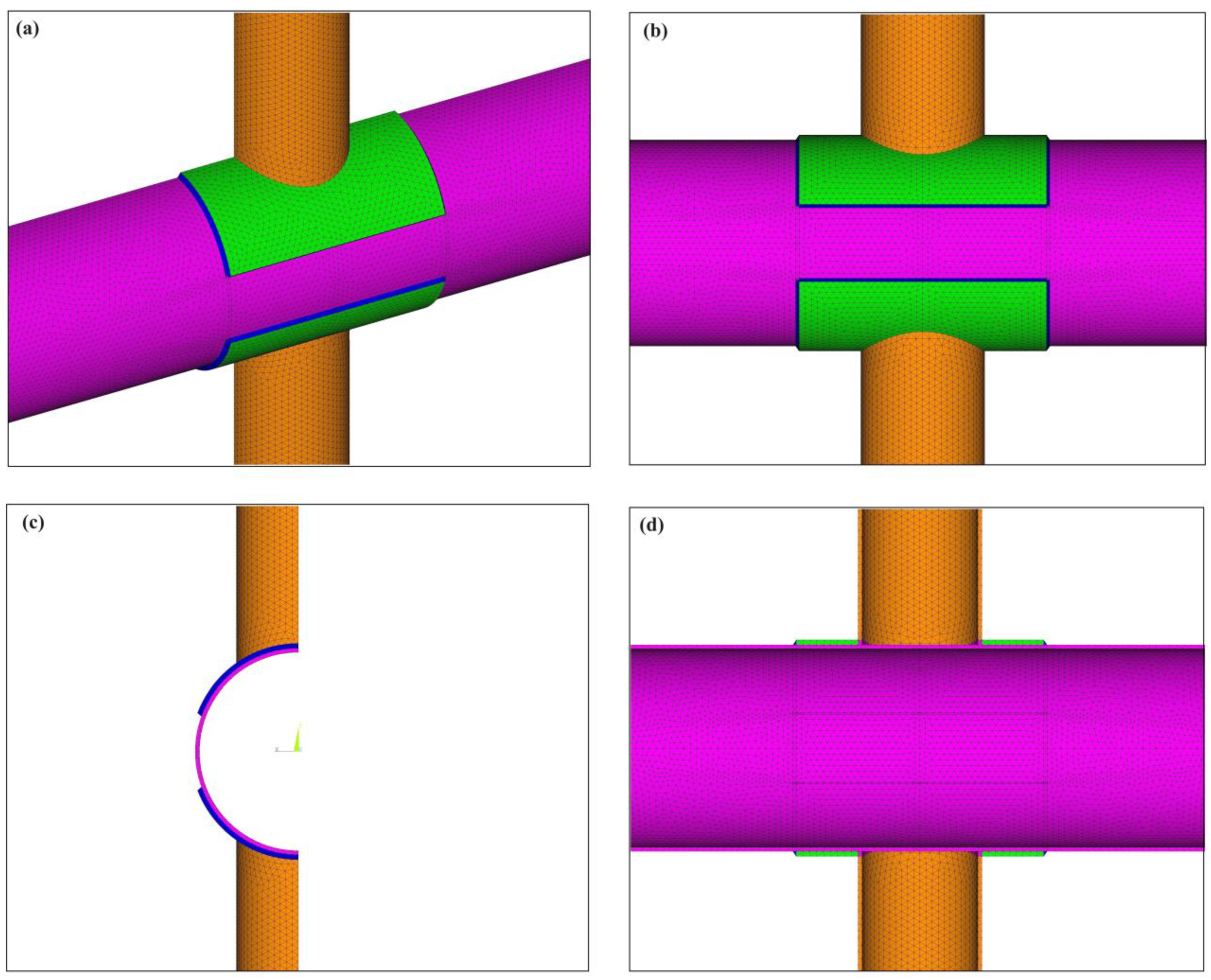
2.1.3. Meshing in ANSYS

The specimens were modeled using the ANSYS SOLID186 element. This element was applied in both unstrengthened and collar plate-reinforced joints during the validation and parametric analyses. The accuracy of the numerical simulations in the validation phase was ensured through the use of tetrahedral elements for FE modeling. Consistent with prior studies investigating the ultimate strength of strengthened tubular nodes under fire conditions [3,12,14], this study opted for tetrahedral elements (SOLID 186) to mesh the joints. Figure 2a–d show the detailed mesh configurations around the collar plate-reinforced section of a tubular X-joint. This approach balances the computational efficiency with the need for accurate simulations. A convergence analysis employing various mesh densities was performed prior to the creation of the 360 FE models designated for the comprehensive parametric study. Regarding the boundary conditions, the displacements at the ends of the main component were restricted in all three axes.

2.1.4. Contact Modeling

In the present study, the technique to facilitate the interaction between the retrofit plates and the tubular node involved the strategic placement of the contact elements. These elements bridged the space between the intended target area, symbolizing the retrofit plate, and the contact zones that encompass the outer planes of the joint. The configuration was distinguished by face-to-face and pliable-to-pliable engagements, preserving a continuous attachment to accurately reflect the interactions between the plates and the joints. This technique guaranteed an authentic representation of the interaction mechanics, achieving a dependable bond between the collars and the joint’s components for the entirety of the modeling process.

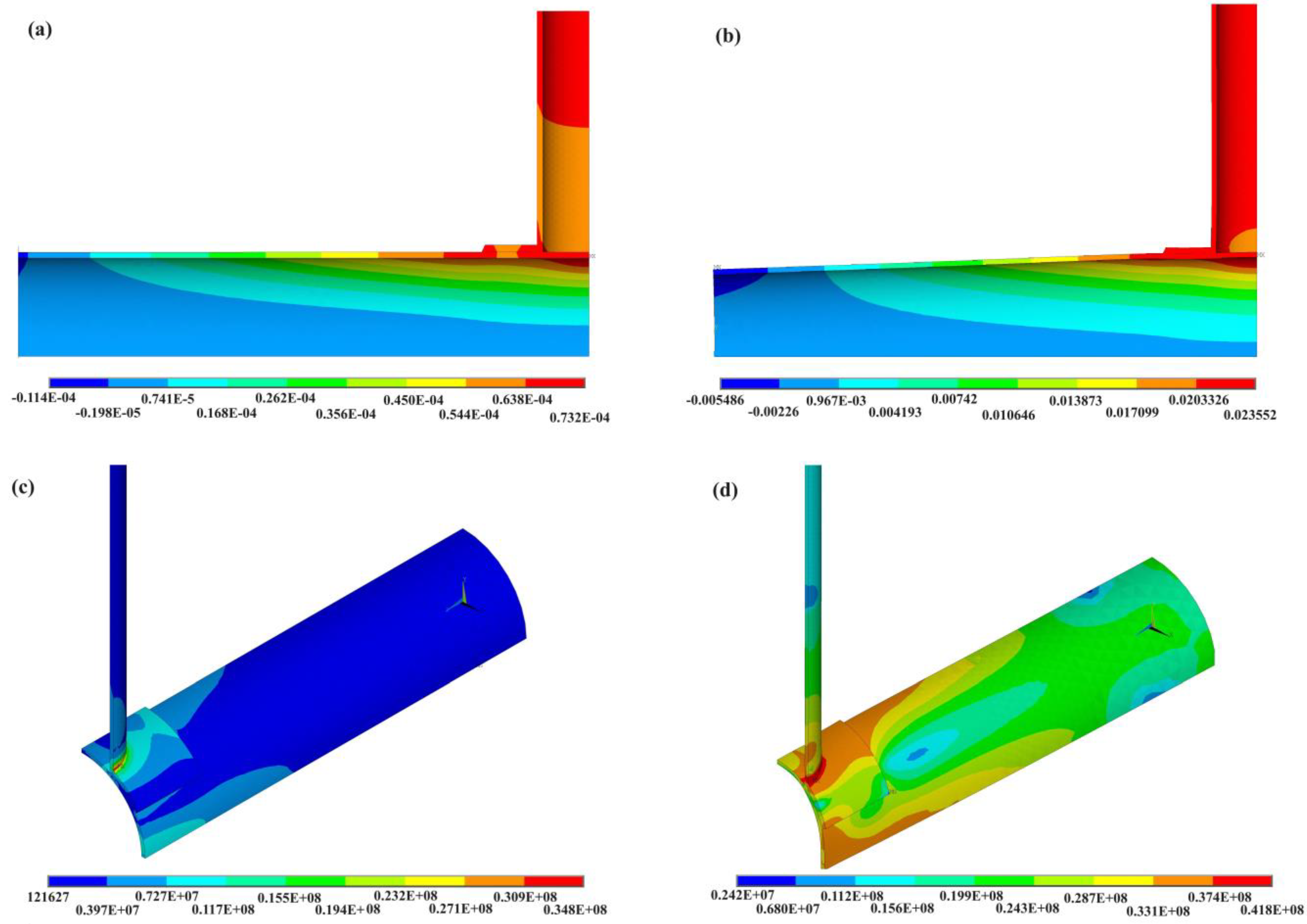
2.1.5. Analysis Method

In this study, the approach to determine the joint capacity under fire conditions involved employing a steady-state analysis. This method entailed subjecting the joint to a load until failure occurred. This methodology aligns with previous research on evaluating the ultimate strength of tubular nodes under fire conditions (references [9,10,12,14]). Additionally, nonlinear material properties and geometric considerations were incorporated into the simulations.

Figure 2. Produced mesh in the strengthened joint intersection. (a,b,d) joint intersection (c) View along the chord’s longitudinal axis. Green color shows the collar plates.

Figure 2. Produced mesh in the strengthened joint intersection. (a,b,d) joint intersection (c) View along the chord’s longitudinal axis. Green color shows the collar plates.

2.2. Resistance Definition

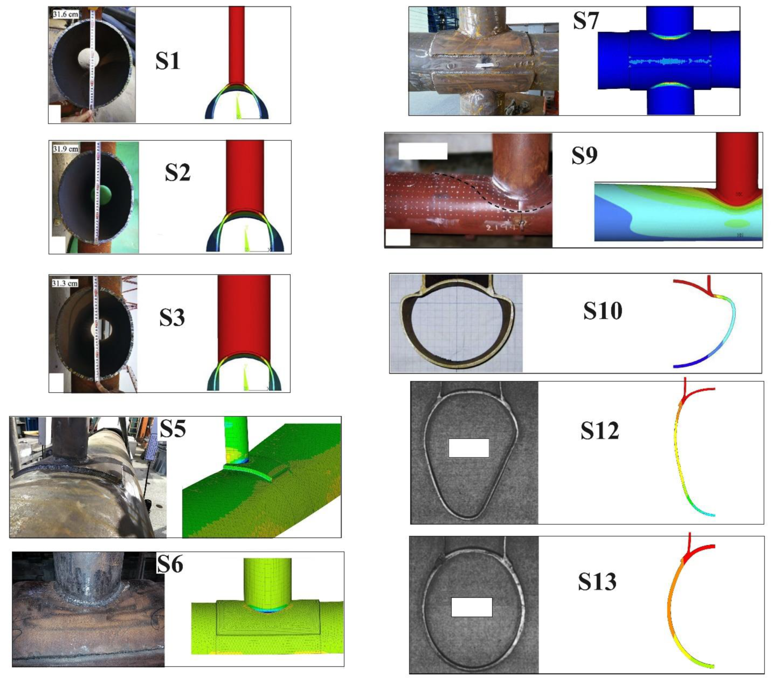
The peak load in load–displacement graphs is considered the ultimate resistance of the joint. However, if the peak occurred after 0.06D (D is the chord diameter), the load on the displacement equal to 0.06D was taken as the ultimate resistance (Choo et al. [6]). It should be noted that generally in the strengthened joints under tension, the displacement limitation occurs before the first peak point.

2.3. FEM Validation

To ensure the fidelity of the FE models, a detailed assessment was conducted by comparing the FE analysis results with those from the relevant experimental studies. Accordingly, the analysis included 31 tests (as detailed in

Table 1. Geometrical variables of the joints for the validation.

Specimen	Researchers	D (m)	d (m)	T (m)	t (m)	tc (m)	δc (m)	Load Type	Temperature
S1	Ding et al. [32]	300	76	7.75	5.87	-	-	Tension	20 °C
S2		300	151	8.11	8.75	-	-
S3		300	219	7.95	8.45	-	-
S4	Shao [4]	0.203	0.5	0.006	0.006	0.006	0.0125	Axial	20 °C
S5	Nassiraei et al. [3]	297.66	160.02	8.63	7.98	8.46	91	Compression	20 °C
S6		297.66	160.02	8.63	7.98	8.46	91
S7		299.95	220.03	8.68	8.19	8.18	77
S8	Tan et al. [9]	0.2445	0.1683	0.0063	0.0063	-	-	Compression	20 °C
S9		0.2445	0.1683	0.0063	0.0063	-	-		550 °C
S10		0.2445	0.1683	0.0063	0.0063	-	-		700 °C
S11		0.2445	0.1956	0.0063	0.0063	-	-		550 °C
S12	Choo et al. [6]	0.4095	0.2219	0.0081	0.0068	0.0064	0.4415	Compression	20 °C
S13		0.4095	0.2214	0.0128	0.0084	0.0083	0.0418
S14		0.4095	0.2219	0.0085	0.0068	0.0064	0.4415	Tension
S15		0.4095	0.2214	0.0128	0.0084	0.0083	0.0418
S16–S23	Ozyurt et al. [10]	0.3239	193.7	0.01	0.01	-	-	Tension	20, 200, 300, 400, 500, 600, 700, 800 °C
S24–S31 *		0.3239	193.7	0.01	0.01	-	-	Tension	20, 200, 300, 400, 500, 600, 700, 800 °C

Note: t_c and δ_c are the collar plate thickness and length, sequentially (see Figure 1) Note: * Brace angle equal to 60°.

and

Table 2. Material parameters.

Specimen	E0 (GPa)	E1 (GPa)	Ec (GPa)	fyo (MPa)	fy1 (MPa)			fyc (MPa)	fuo (MPa)	fu1 (MPa)	fuc (MPa)
S1	200.3	222.3	-	267.7	313.3			-	-	-	-
S2	200.3	240	-	267.7	295			-	-	-	-
S3	200.3	244.3	-	267.7	317.7			-	-	-	-
S4	200	200	200	321	389			348	480	576	516
S5	206	218	213.3	270	358			285	460	470	474
S6	206	209	213.3	270	280			285	460	457	474
S7	206	203	213.3	270	298			285	460	469	474
S8	201	201	-	380.3	380.3			-	519.1	519.1	-
S9	The specifications for the material properties under high-temperature conditions are delineated following Equations (2)–(9) as outlined in EN 1993-1-2 [30].
S10
S11
S12	205	205	205	285		300	461		-	-	-
S13	205	205	205	276		275	464		-	-	-
S14	205	205	205	276		300	461		-	-	-
S15	205	205	205	276		275	464		-	-	-
S16	210	210	-	355		355	-		-	-	-
S17–S23	The specifications for the material properties under high-temperature conditions are delineated following Equations (2)–(9) as outlined in EN 1993-1-2 [30].
S24	210	210	-	355		355	-		-	-	-
S25–S31	The specifications for the material properties under high-temperature conditions are delineated following Equations (2)–(9) as outlined in EN 1993-1-2 [30].

): three experiments on CHS X-joints under tensile loading by Ding et al. [32], a single CHS T-joint strengthened with a retrofit plate conducted by Shao [4], three instances of CHS X-joints equipped with retrofit plates under compressive stress, undertaken by the author of this study [3], four T-joints under standard temperature conditions and various elevated temperatures as documented by Tan et al. [9], four T-joints with collar plates conducted by Choo et al. [6], and 16 tests of X-joints under tensile loading at different elevated temperatures carried out by Ozyurt et al. [10].

The load–displacement of the FEM and experimental tests are depicted in Figure 3. S1–S3 illustrate the finding of three unstrengthened CHS X-joints under brace tension. S4 reveals the findings for T-joints strengthened with the retrofitting plates under brace tension. Additionally, S5–S7 exhibit the findings for CHS X-joints with the retrofitting plates under brace compression. Finally, S8–S11 reveal the compression for T-joints under ambient and fire conditions.

The response patterns from S1 to S11 demonstrate the capability of the current finite element model (FEM) to accurately predict the performance of CHS joints, both with and without the addition of strengthening plates, under normal and elevated temperature conditions. A detailed comparison of the peak load capacities between the FEM predictions and actual experimental and numerical outcomes from all 31 tests is presented in

Table 3. Numerical versus empirical results: a comparative study.

Specimen	Fu,test (kN)	Fu,num (kN)	Fu,num/Fu,test
S1	188.2	183.8	0.98
S2	265.3	287.1	1.08
S3	418	436.4	1.04
S4	147.46	166.3	1.13
S5	272.2	258	0.95
S6	366.2	404	1.10
S7	529.1	572	1.08
S8	338	339	1.0
S9	175.2	171.7	0.98
S10	55	55.6	1.01
S11	216	218	1.0
S12	425.6	441.3	1.04
S13	780	812.2	1.04
S14	609.2	684.5	1.12
S15	1065.3	1111.3	1.04

and

Table 4. Comparison between F_{u,elevated temperature} and F_{u,20 °C}.

Specimen	Ozyurt et al. [10]	Present Study	Present Study/Ozyurt et al. [10]
S16	1	1	1
S17	0.97	0.98	1.01
S18	0.93	0.95	1.02
S19	0.91	0.95	1.04
S20	0.72	0.74	1.03
S21	0.43	0.45	1.05
S22	0.20	0.22	1.10
S23	0.10	0.10	1.0
S24	1.0	1.0	1.0
S25	1.0	1.0	1.0
S26	1.0	1.0	1.0
S27	1.0	1.0	1.0
S28	0.80	0.82	1.03
S29	0.48	0.51	1.06
S30	0.21	0.22	1.05
S31	0.11	0.12	1.09

. This comparison indicates a notable alignment between the FEM predictions and the other experimental and numerical data. Also, Figure 4 shows that the present FE model can predict the failure modes well. Consequently, the analysis derived from Figure 3 and Figure 4, and the data in Table 3 and Table 4 validate the effectiveness of the proposed model in precisely evaluating the ultimate resistance of CHS joints strengthened by retrofitting plates, across both ambient conditions and in the presence of fire.

2.4. Database Organization

According to Section 2.1, Section 2.2 and Section 2.3, 360 CHS X-joints with the retrofitting plates (

Table 5. Parameters for the dimensional and non-dimensional analysis in the parametric assessment.

Parameter	Expression	Value(s)
η	δc/d	0.25, 0.50, 0.75, 1.00
τc	tc/T	1.00, 1.25, 1.50, 1.75
β	d/D	0.2, 0.4, 0.5, 0.6, 0.8
γ	D/2T	10, 18, 20, 26
τ	t/T	0.7, 1.0
D	Chord diameter	0.3 m
T	Temperature	20 °C, 200 °C, 400 °C, 600 °C, 800 °C

) were modeled and analyzed. A database was created using the ultimate resistance values. This database included Datasets 1 through 5, which sequentially recorded the resistance values of X-joints featuring a tensioned plate at temperatures of 20, 200, 400, 600, and 800 degrees Celsius. Demonstrated in Figure 5 is the altered configuration of an X-joint that has been strengthened with a retrofitting plate at a temperature of 600 °C. Figure 6 shows the deformed shapes of a collar plate-strengthened X-joint with β = 0.5, γ = 18, τ = 1, η = 0.5, and τ_c = 1.25 at 400 and 800 °C. The same load was applied for both of the elevated temperatures. Figure 6a,b depict the vertical displacement in the joints at 400 and 800 °C, respectively. Also, Figure 6c,d show the von mises stress in the joints at 400 and 800 °C, respectively. As the temperature rises, the capacity of the steel structures decreases due to the reduced steel strength. This decrease in strength leads to a reduced stiffness in both the chord and plate components of the structure. Moreover, the connection capacity was notably affected by temperature increases, especially beyond 400 °C, because the strength of joints is closely tied to the yield stress (fy). According to Eurocode EN-1993-1-2 [30], as listed in Table 3.1, at temperatures exceeding 400 °C, the yield stress (fy) of steel members decreases significantly as a result of elevated temperature effects. Consequently, the overall capacity of the structure was significantly diminished at temperatures above 400 °C. Figure 6 illustrates that higher temperatures correspond to increased displacement and stress within the structure. The maximum displacement happened in the joints at 400 and 800 °C and was equal to 0.0007 and 0.0235 m. Moreover, at 800 °C (Figure 6d) almost the whole of the chord and collar was under high stress values. But, at 400 °C (Figure 6c) just the chord and collar in the joint’s intersection were under high stress values. Also, the maximum stress in the joints at 400 and 800 °C was equal to 34.8 and 41.8 MPa.

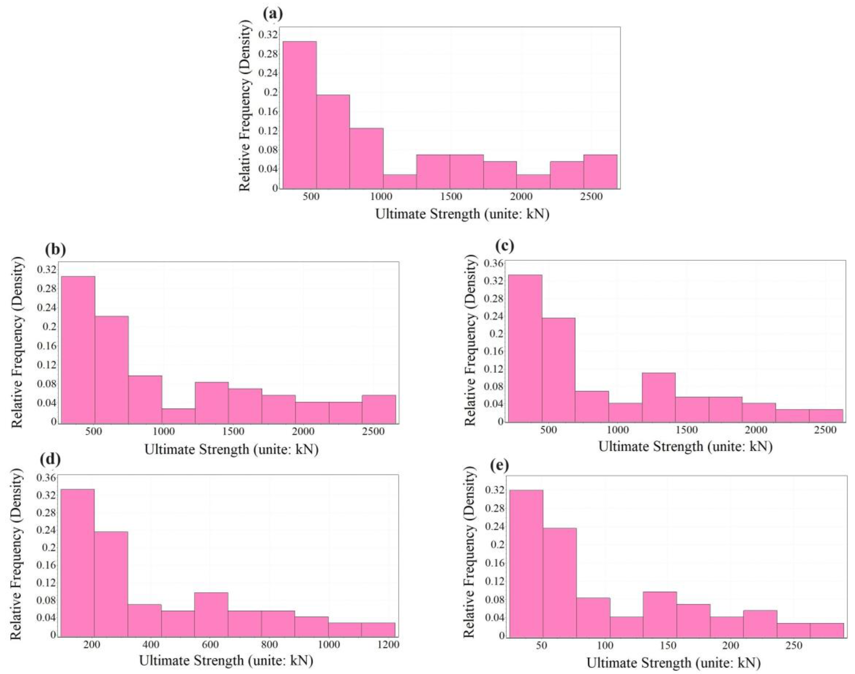
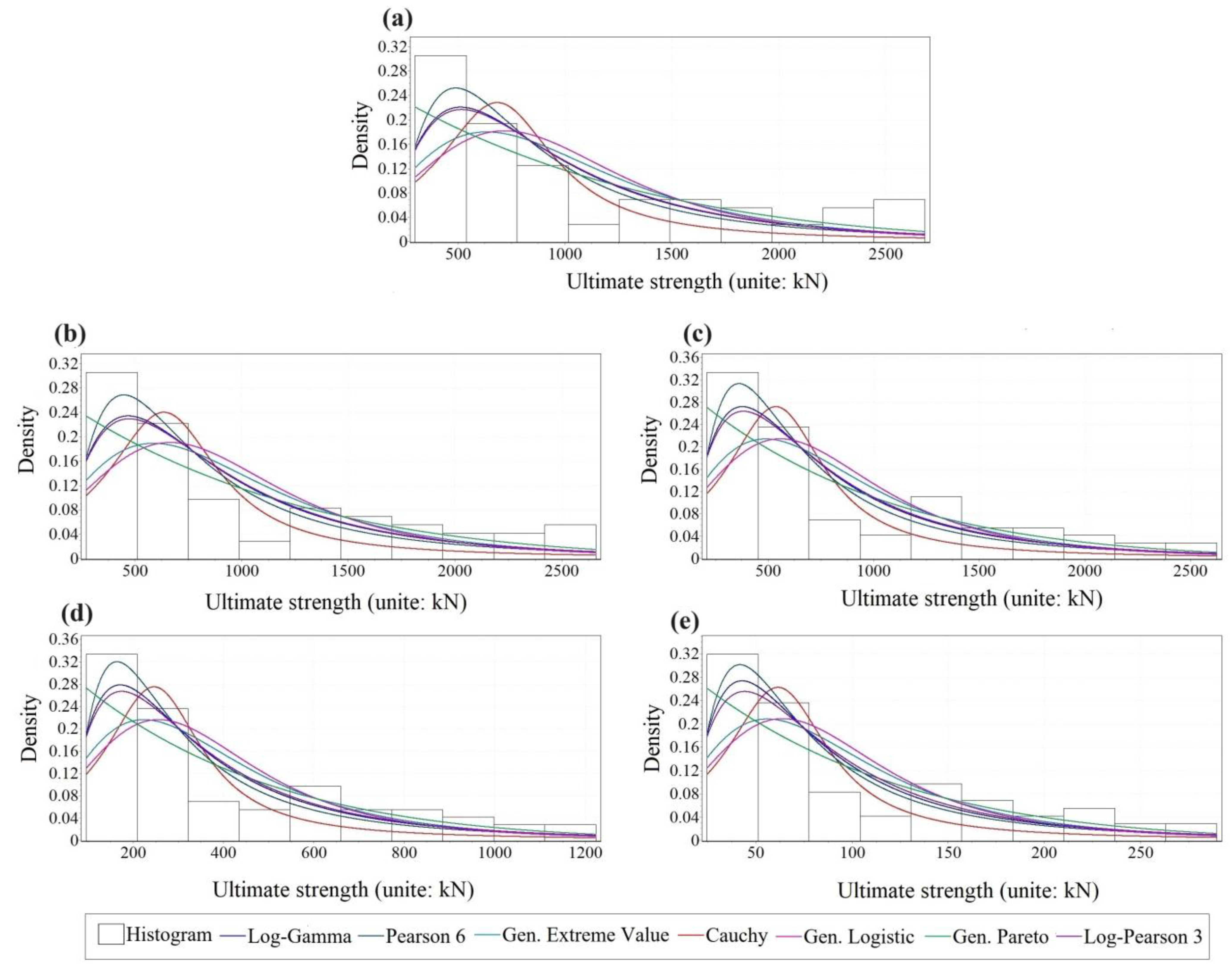
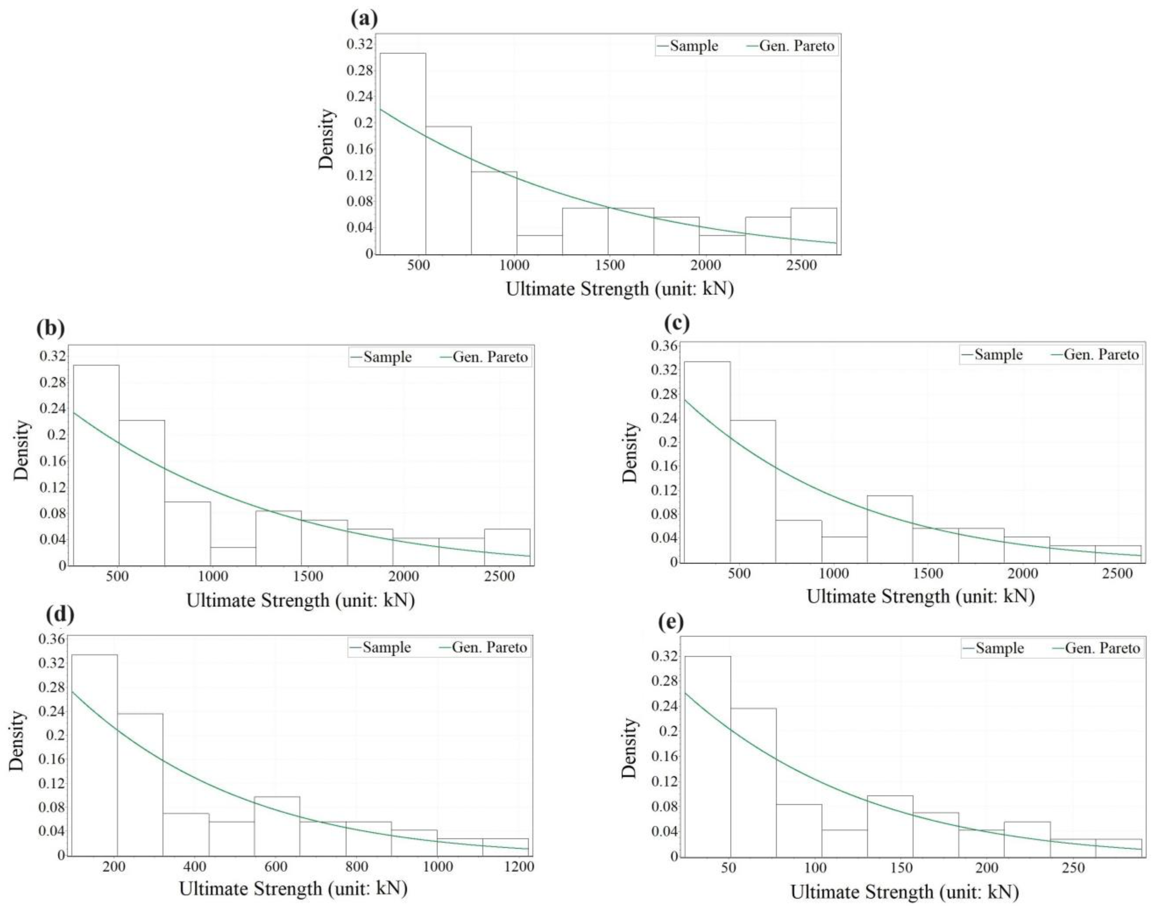
2.5. Density Histogram Generation

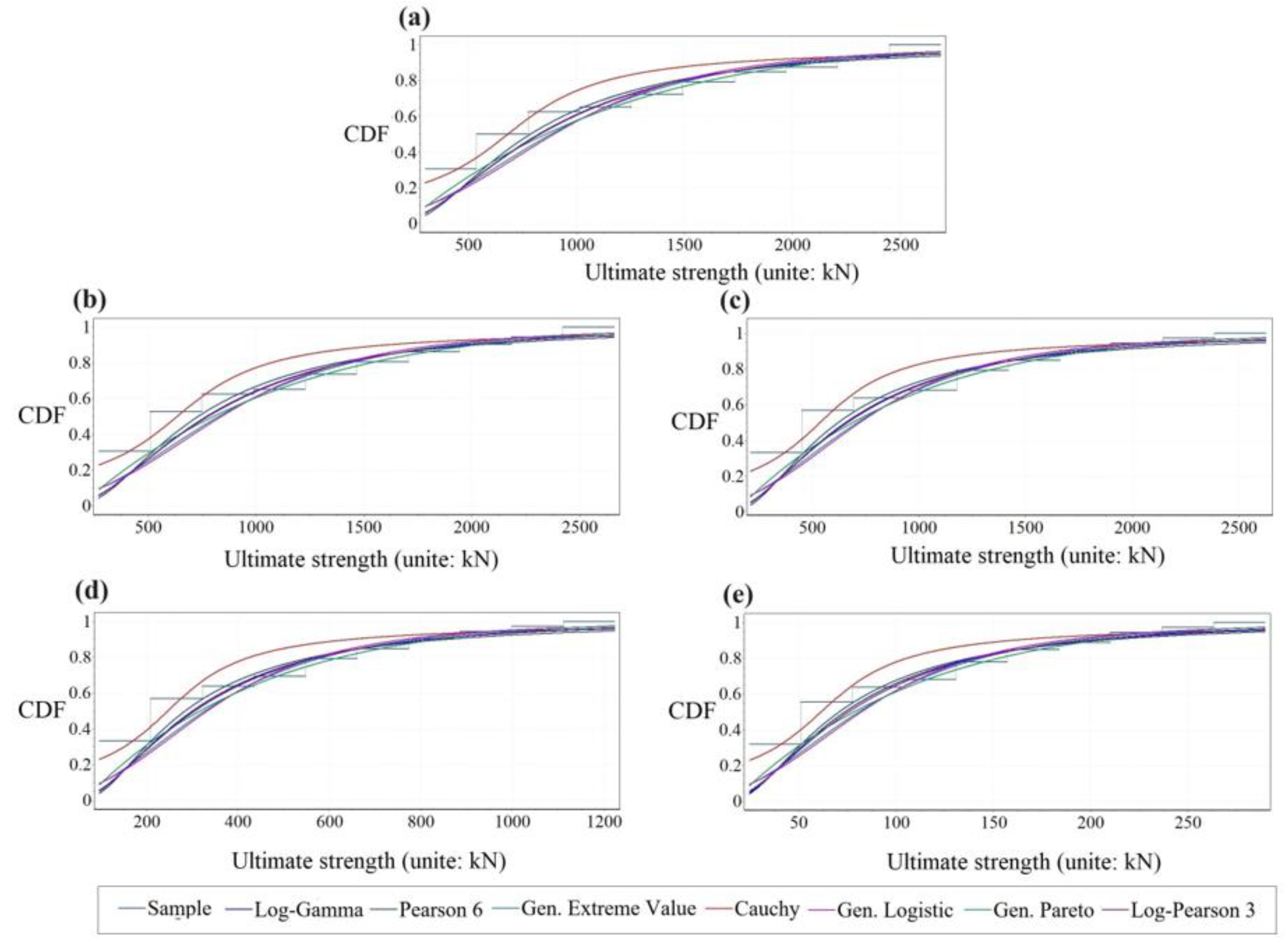
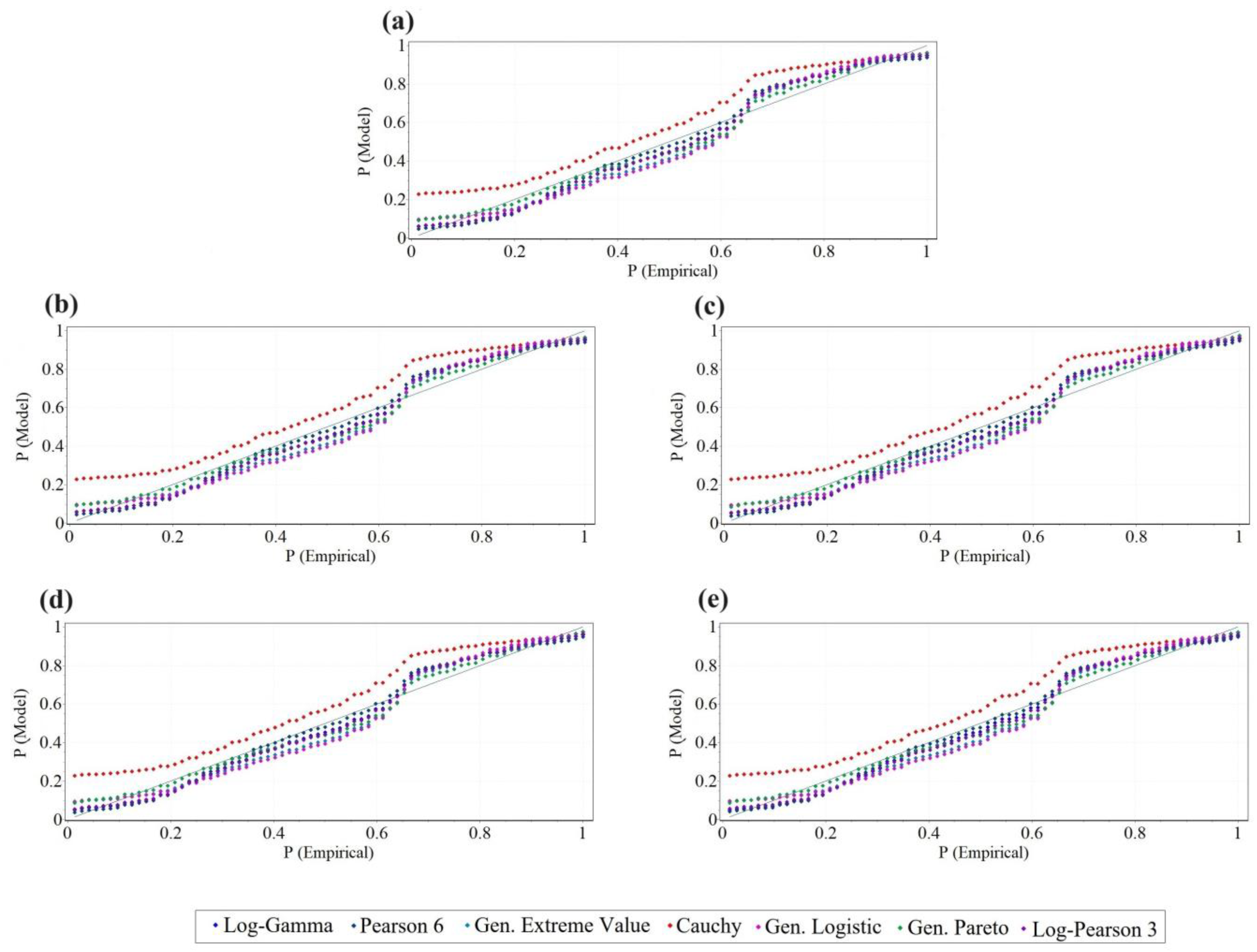
To exhibit the distribution of the databases, the histograms should be plotted. Therefore, the dataset range (ultimate resistance values) was segmented into several groups, n_g. Subsequently, the frequencies (the count of occurrences in each group) were identified. In the next stage, the relative frequency for each group was calculated. For more details, the reader can refer to Nassiraei [14]. Following this, the density for each group was established. Figure 7 showcases the density histograms for the five datasets. The statistical outcomes for the five generated samples are detailed in

Table 6. Statistical analysis of the sampled data for the joints.

	Statistical Measure	Symbol	Unit	Database 1	Database 2	Database 3	Database 4	Database 5
Sample size	-	n	-	72	72	72	72	72
Measures of central tendency	Mean	μ	kN	1061.4	1004.1	879.96	406.0	99.471
	Median	-	-	767.98	715.9	609.9	279.3	69.5
	Interquartile range	iqr	kN	1115.63	1072.95	971.63	452.42	108.6
	Std. Deviation	σ	kN	719.25	696.58	643.47	298.69	71.861
	Coef. of Variation	ν	-	0.67764	0.69374	0.73124	0.73569	0.72243

.

Figure 6. The effect of temperature on the deformed shape and stress: (a,b) displacement in vertical axis (unit: m); (c,d) von mises stress (unit: Pa).

Figure 6. The effect of temperature on the deformed shape and stress: (a,b) displacement in vertical axis (unit: m); (c,d) von mises stress (unit: Pa).

Figure 7. The histograms produced for the ultimate resistance of the joints: (a) 20, (b) 200, (c) 400, (d) 600, (e) 800 °C.

Figure 7. The histograms produced for the ultimate resistance of the joints: (a) 20, (b) 200, (c) 400, (d) 600, (e) 800 °C.

3. PDF Fitting

A lot of theoretical models were fitted to the results. After that, just 12 PDFs that most accurately reflected the histogram densities were listed. The PDFs were leveraged to analyze the data represented in the histograms. For visual clarity and effectiveness, Figure 8 selectively showcases only those PDFs that most accurately reflect the histogram densities. In contrast, Figure 9 portrays how the calculated continuous CDFs correspond with the empirical distribution functions (EDFs) derived from the data collection. Additionally, the relationship between the theoretical and observed CDFs is critically evaluated through probability–probability plots in Figure 10.

For parameter estimation within these twelve distributions, the strategy of Maximum Likelihood Estimation (MLE) was adopted. This technique is designed to identify the most probable parameters of a distribution, denoted as f_X(x), based on a set of empirical observations x₁, x₂, …, x_n from a test with n entries. It hinges on MLE that encapsulates the parameter θ:

$$L(\theta )=L(x_1,x_2,\dots ,x_n)={\displaystyle \prod }_{i=1}^{n}f(x_i;\theta )$$

(12)

In Equation (12), θ is the vector of unspecified variables. This approach was employed across various parametric models, encompassing the Gen. Extreme Value, Gen. Pareto, Cauchy, Log-Gamma, Frechet, Weibull, Gen. Logistic, Gumbel Max, Log-Logistic, Inv. Gaussian, Log-Pearson 3, and Pearson 6. By using the findings of the plate-retrofitted X-joint models,

Table 7. Estimated variables for the PDFs shaped to the density histograms of the samples for the joints.

#	Distribution	Continuous Variables	Estimated Values
			Database 1	Database 2	Database 3	Database 4	Database 5
1	Cauchy	μ	683.27	635.32	536.59	246.47	61.44
		σ	332.22	316.56	282.45	130.43	32.119
2	Frechet	α	1.701	1.6637	1.5813	1.5704	1.597
		β	600.66	557.52	466.87	214.11	53.282
3	Generalized Extreme Value	μ	698.45	651.47	552.87	254.14	62.986
		σ	491.45	469.48	420.47	194.6	47.416
		k	0.14147	0.15091	0.17037	0.17212	0.16434
4	Generalized Logistic	μ	895.47	840.1	722.58	332.71	82.097
		σ	351.47	337.55	305.62	141.59	34.348
		k	0.26413	0.27066	0.28421	0.28543	0.27999
5	Generalized Pareto	μ	205.87	183.72	139.06	62.824	16.143
		σ	996.03	941.78	825.93	381.54	93.746
		k	−0.16423	−0.14797	−0.11475	−0.11179	−0.12502
6	Gumbel Max	μ	737.7	690.6	590.37	271.57	67.13
		σ	560.8	543.13	501.71	232.89	56.03
7	Inv. Gaussian	μ	1061.4	1004.1	879.96	406.0	99.471
		λ	2311.4	2086.3	1645.7	750.13	190.59
8	Log-Gamma	α	97.239	90.818	77.628	59.407	35.213
		β	0.06932	0.07349	0.08394	0.09661	0.1233
9	Log-Logistic	α	2.4135	2.3612	2.2487	2.2332	2.2704
		β	832.39	778.29	663.16	304.88	75.425
10	Log-Pearson 3	α	186.22	192.3	230.62	237.83	246.75
		β	0.05009	0.0505	0.0487	0.04828	0.04658
		γ	−2.5874	−3.0377	−4.7152	−5.7441	−7.1517
11	Pearson 6	α1	166.55	114.75	112.32	351.6	54.099
		α2	2.5167	2.4283	2.187	2.1397	2.2693
		β	10.387	13.482	10.36	1.4734	2.5637
12	Weibull	α	1.6667	1.6307	1.5553	1.5446	1.5702
		β	1161.3	1093.8	947.53	436.69	107.4

lists the variables of the distributions.

4. Investigating the PDFs

4.1. Kolmogorov–Smirnov (K-S) Assessment

The Kolmogorov–Smirnov (K-S) test was utilized to determine the peak divergence in a vertical sense between the theoretical and the empirical CDFs. In relation to resistance data points x₁, x₂, …, x_n, the formulation for the empirical CDF is as outlined subsequently:

$$F_n(x)=\frac{1}{n}[n(i)]\hspace{0.17em}$$

(13)

In this context, n signifies the size of the dataset under consideration. The term n_(i) denotes the count of data points that are less than the value of x_i, with the x_i values arranged in ascending order. The calculation of the Kolmogorov–Smirnov (K–S) statistic, represented by D, was performed as follows:

$$D_n={\max }_{1\le i\le n}[F(x_i)-\frac{i-1}{n},\frac{i}{n}-F(x_i)]$$

(14)

For sample sizes n ≥ 40, the threshold of acceptability can be determined through Equation (15) (Kottegoda et al. [33]). ξ is the alpha risk. It demonstrates the level of significance.

$$\begin{array}{l}If \xi =0.01 \Rightarrow D_{n,\xi }=\frac{1.6276}{\sqrt{n}}\\ If \xi =0.05 \Rightarrow D_{n,\xi }= \frac{1.3581}{\sqrt{n}}\end{array}$$

(15)

The Kolmogorov–Smirnov (K–S) analysis was conducted to examine the load capacity of X-joint configurations with the plates, across a range of environmental temperatures. The results are compiled in

Table 8. Assessment of the models against the K-S test criteria for database 1.

#	Distribution	Statistic	α = 0.05		α = 0.01		Rank
			Critical Value	Finding	Critical Value	Finding
1	Cauchy	0.22733	0.15755	Fail	0.18903	Fail	12
2	Frechet	0.11633		OK		OK	9
3	Generalized Extreme Value	0.09585		OK		OK	4
4	Generalized Logistic	0.1087		OK		OK	8
5	Generalized Pareto	0.09085		OK		OK	1
6	Gumbel Max	0.12942		OK		OK	11
7	Inv. Gaussian	0.09703		OK		OK	5
8	Log-Gamma	0.09548		OK		OK	3
9	Log-Logistic	0.09937		OK		OK	6
10	Log-Pearson 3	0.09369		OK		OK	2
11	Pearson 6	0.10851		OK		OK	7
12	Weibull	0.12238		OK		OK	10

,

Table 9. Assessment of the models against the K-S test criteria for database 2.

#	Statistic	α = 0.05		α = 0.01		Rank
		Critical Value	Finding	Critical Value	Finding
1	0.22814	0.15755	Fail	0.18903	Fail	12
2	0.11606		OK		OK	9
3	0.09562		OK		OK	3
4	0.10839		OK		OK	7
5	0.09008		OK		OK	1
6	0.13215		OK		OK	11
7	0.09833		OK		OK	5
8	0.09588		OK		OK	4
9	0.10028		OK		OK	6
10	0.09432		OK		OK	2
11	0.1092		OK		OK	8
12	0.12215		OK		OK	10

,

Table 10. Assessment of the models against the K–S test criteria for Database 3.

#	Statistic	α = 0.05		α = 0.01		Rank
		Critical Value	Finding	Critical Value	Finding
1	0.22745	0.15755	Fail	0.18903	Fail	12
2	0.1168		OK		OK	9
3	0.09798		OK		OK	3
4	0.11068		OK		OK	8
5	0.08382		OK		OK	1
6	0.13453		OK		OK	11
7	0.09955		OK		OK	4
8	0.09957		OK		OK	5
9	0.10522		OK		OK	6
10	0.0974		OK		OK	2
11	0.10906		OK		OK	7
12	0.12021		OK		OK	10

,

Table 11. Assessment of the models against the K–S test criteria for database 4.

#	Statistic	α = 0.05		α = 0.01		Rank
		Critical Value	Finding	Critical Value	Finding
1	0.22796	0.15755	Fail	0.18903	Fail	12
2	0.11813		OK		OK	9
3	0.09893		OK		OK	3
4	0.11165		OK		OK	7
5	0.08512		OK		OK	1
6	0.13555		OK		OK	11
7	0.10123		OK		OK	4
8	0.10179		OK		OK	5
9	0.10652		OK		OK	6
10	0.09834		OK		OK	2
11	0.11212		OK		OK	8
12	0.12058		OK		OK	10

and

Table 12. Assessment of the models against the K–S test criteria for database 5.

#	Statistic	α = 0.05		α = 0.01		Rank
		Critical Value	Finding	Critical Value	Finding
1	0.22824	0.15755	Fail	0.18903	Fail	12
2	0.11578		OK		OK	9
3	0.09362		OK		OK	2
4	0.1073		OK		OK	7
5	0.08673		OK		OK	1
6	0.13288		OK		OK	11
7	0.10166		OK		OK	5
8	0.1011		OK		OK	4
9	0.1038		OK		OK	6
10	0.09618		OK		OK	3
11	0.10866		OK		OK	8
12	0.11777		OK		OK	10

. The insights from the K–S evaluation highlight that the Generalized Petro model demonstrates the minimal test statistical value for joints under tensile stress under varying thermal conditions (20, 200, 400, 600, and 800 °C), as detailed in Table 8, Table 9, Table 10, Table 11 and Table 12. Therefore, the analysis suggests that the Generalized Petro model consistently provides the most accurate predictive performance for the structural integrity at diverse temperature settings.

4.2. Anderson–Darling (A-D) Assessment

Critical values are available in the Handbook by Stephens [34]. The Anderson–Darling test’s statistic (Hu et al. [35]) is:

$$AD=-n-\frac{1}{n}{\displaystyle \sum _{i=1}^n(2i-1)[\ln F(X_i)+\ln (1-F(X_{n-i+1}))]}\hspace{0.17em}$$

(16)

In Equation (16), F is the CDF of the distribution. Additionally, X_i is the ordered data.

The shaped PDFs were evaluated according to the A–D trial. The findings are detailed in

Table 13. Assessment of the models against the A–D test criteria for database 1.

#	Distribution	Statistic	α = 0.05		α = 0.01		Rank
			Critical Value	Finding	Critical Value	Finding
1	Cauchy	5.9451	2.5018	Fail	3.9074	Fail	12
2	Frechet	1.1578		OK		OK	5
3	Generalized Extreme Value	1.5063		OK		OK	7
4	Generalized Logistic	1.9315		OK		OK	8
5	Generalized Pareto	0.8553		OK		OK	1
6	Gumbel Max	1.9739		OK		OK	10
7	Inv. Gaussian	1.9358		OK		OK	9
8	Log-Gamma	1.1054		OK		OK	3
9	Log-Logistic	1.2212		OK		OK	6
10	Log-Pearson 3	1.1215		OK		OK	4
11	Pearson 6	1.1052		OK		OK	2
12	Weibull	2.0589		OK		OK	11

,

Table 14. Assessment of the models against the A–D test criteria for database 2.

#	Statistic	α = 0.05		α = 0.01		Rank
		Critical Value	Finding	Critical Value	Finding
1	6.0555	2.5018	Fail	3.9074	Fail	12
2	1.1457		OK		OK	5
3	1.4833		OK		OK	7
4	1.905		OK		OK	8
5	0.82676		OK		OK	1
6	1.97		OK		OK	19
7	1.9464		OK		OK	9
8	1.0665		OK		OK	2
9	1.197		OK		OK	6
10	1.084		OK		OK	4
11	1.0829		OK		OK	3
12	2.0118		OK		OK	11

,

Table 15. Assessment of the models against the A–D test criteria for database 3.

#	Statistic	α = 0.05		α = 0.01		Rank
		Critical Value	Finding	Critical Value	Finding
1	6.2353	2.5018	Fail	3.9074	Fail	12
2	1.1133		OK		OK	5
3	1.4145		OK		OK	7
4	1.8219		OK		OK	8
5	0.75897		OK		OK	1
6	1.9492		OK		OK	10
7	1.9521		OK		OK	11
8	0.95889		OK		OK	2
9	1.1182		OK		OK	6
10	0.9794		OK		OK	3
11	0.98753		OK		OK	4
12	1.9005		OK		OK	9

,

Table 16. Assessment of the models against the A–D test criteria for database 4.

#	Statistic	α = 0.05		α = 0.01		Rank
		Critical Value	Finding	Critical Value	Finding
1	6.2595	2.5018	Fail	3.9074	Fail	12
2	1.1364		OK		OK	6
3	1.4229		OK		OK	7
4	1.8292		OK		OK	8
5	0.77009		OK		OK	1
6	1.9613		OK		OK	10
7	1.9884		OK		OK	11
8	0.96404		OK		OK	2
9	1.1215		OK		OK	5
10	0.98715		OK		OK	3
11	1.0092		OK		OK	4
12	1.8943		OK		OK	9

and

Table 17. Assessment of the models against the A–D test criteria for database 5.

#	Statistic	α = 0.05		α = 0.01		Rank
		Critical Value	Finding	Critical Value	Finding
1	6.0958	2.5018	Fail	3.9074	Fail	12
2	1.1436		OK		OK	6
3	1.4038		OK		OK	7
4	1.8102		OK		OK	8
5	0.75742		OK		OK	1
6	1.9126		OK		OK	10
7	1.9581		OK		OK	11
8	0.96931		OK		OK	2
9	1.1199		OK		OK	5
10	0.9923		OK		OK	3
11	1.0106		OK		OK	4
12	1.878		OK		OK	9

. This comparison shows that, for X-joints strengthened with retrofitting plates across various ambient and higher temperature conditions, the Generalized Petro distribution emerges as the superior model. This conclusion is drawn because its test statistical values are consistently the lowest across all temperature ranges, as documented in Table 13, Table 14, Table 15, Table 16 and Table 17.

4.3. Chi-Squared (C-S) Assessment

It is deemed safe to proceed when the test statistic follows a Cramer-von Mises distribution under the null hypothesis. Equation (16) is utilized to evaluate the disparity between theoretical and empirical information.

$$X^2={\displaystyle \sum _{i=1}^{n_c}\frac{{(O_i-E_i)}^2}{E_i}}$$

(17)

where O_i indicates the observed frequencies, and E_i represents the expected frequencies. A high-test statistic value indicates a lack of alignment between the model and the data. The rejecting value is ${\chi }_{1-\xi ,v}^2$, where v = n_c − k − 1 reveals the degrees of freedom. Additionally, k presets the estimated variables number. ${\chi }_{1-\xi ,v}^2$ represents the threshold at which a C-S variable X surpasses with a probability of ξ, specifically:

$$\begin{array}{l}\mathrm{Pr}[X\le {\chi }_{1-\xi ,\nu }^2]={\displaystyle {\int }_0^{{\chi }_{1-\xi ,\nu }^2}{f}_X(x)dx=1-\xi }\\ f_X(x)=\left\{\begin{array}{l}\frac{1}{2^{\nu /2}\mathsf{\Gamma }(\nu /2)}{x}^{(\nu -2)/2}{e}^{-x/2}\hspace{0.17em}\hspace{0.17em}\hspace{0.17em}\hspace{0.17em}\hspace{0.17em}\hspace{0.17em}\hspace{0.17em}\hspace{0.17em}\hspace{0.17em}\hspace{0.17em}\hspace{0.17em}\hspace{0.17em}\hspace{0.17em}\hspace{0.17em}\hspace{0.17em}\hspace{0.17em}x\ge 0\\ 0\hspace{0.17em}\hspace{0.17em}\hspace{0.17em}\hspace{0.17em}\hspace{0.17em}\hspace{0.17em}\hspace{0.17em}\hspace{0.17em}\hspace{0.17em}\hspace{0.17em}\hspace{0.17em}\hspace{0.17em}\hspace{0.17em}\hspace{0.17em}\hspace{0.17em}\hspace{0.17em}\hspace{0.17em}\hspace{0.17em}\hspace{0.17em}\hspace{0.17em}\hspace{0.17em}\hspace{0.17em}\hspace{0.17em}\hspace{0.17em}\hspace{0.17em}\hspace{0.17em}\hspace{0.17em}\hspace{0.17em}\hspace{0.17em}\hspace{0.17em}\hspace{0.17em}\hspace{0.17em}\hspace{0.17em}\hspace{0.17em}\hspace{0.17em}x<0\end{array}\right.\\ \mathsf{\Gamma }(\nu /2)={\displaystyle \underset{0}{\overset{\infty }{\int }}{x}^{(\nu /2)-1}{e}^{-x}dx}\end{array}$$

(18)

Table 18. Assessment of the models against the C-S test criteria for database 1.

#	Distribution	Statistic	α = 0.05		α = 0.01		Rank
			Critical Value	Finding	Critical Value	Finding
1	Cauchy	5.8114	11.07	OK	15.086	OK	2
2	Frechet	8.1841		OK		OK	7
3	Generalized Extreme Value	7.6429		OK		OK	5
4	Generalized Logistic	9.192		OK		OK	10
5	Generalized Pareto	3.9917		OK		OK	1
6	Gumbel Max	9.348		OK		OK	11
7	Inv. Gaussian	9.1666		OK		OK	9
8	Log-Gamma	5.9697		OK		OK	3
9	Log-Logistic	9.003		OK		OK	8
10	Log-Pearson 3	7.0805		OK		OK	4
11	Pearson 6	8.1147		OK		OK	6
12	Weibull	10.974		OK		OK	12

,

Table 19. Assessment of the models against the C-S test criteria for database 2.

#	Statistic	α = 0.05		α = 0.01		Rank
		Critical Value	Finding	Critical Value	Finding
1	6.0562	11.07	OK	15.086	OK	4
2	6.8167		OK		OK	6
3	6.2811		OK		OK	5
4	9.4801		OK		OK	9
5	4.136		OK		OK	1
6	10.363		OK		OK	12
7	9.61		OK		OK	10
8	4.9555		OK		OK	2
9	9.3863		OK		OK	8
10	5.7531		OK		OK	3
11	8.4904		OK		OK	7
12	10.281		OK		OK	11

,

Table 20. Assessment of the models against the C-S test criteria for database 3.

#	Statistic	α = 0.05		α = 0.01		Rank
		Critical Value	Finding	Critical Value	Finding
1	8.0775	11.07	OK	15.086	OK	8
2	6.7643		OK		OK	6
3	5.3979		OK		OK	3
4	12.016		Fail		OK	11
5	4.5525		OK		OK	1
6	12.139		Fail		OK	12
7	9.1876		OK		OK	9
8	5.041		OK		OK	2
9	7.6378		OK		OK	7
10	6.3252		OK		OK	5
11	5.4001		OK		OK	4
12	11.728		Fail		OK	10

,

Table 21. Assessment of the models against the C-S test criteria for database 4.

#	Statistic	α = 0.05		α = 0.01		Rank
		Critical Value	Finding	Critical Value	Finding
1	8.1476	11.07	OK	15.086	OK	7
2	8.3311		OK		OK	8
3	5.4128		OK		OK	3
4	12.026		Fail		OK	10
5	4.5739		OK		OK	1
6	12.141		Fail		OK	11
7	10.245		OK		OK	9
8	4.773		OK		OK	2
9	7.653		OK		OK	6
10	6.3394		OK		OK	5
11	5.8302		OK		OK	4
12	12.495		Fail		OK	12

and

Table 22. Assessment of the models against the C-S test criteria for database 5.

#	Statistic	α = 0.05		α = 0.01		Rank
		Critical Value	Finding	Critical Value	Finding
1	6.6775	11.07	OK	15.086	OK	6
2	7.6284		OK		OK	8
4	4.6218		OK		OK	2
5	11.88		Fail		OK	11
6	3.3767		OK		OK	1
7	13.367		Fail		OK	12
8	10.6		OK		OK	9
9	5.8354		OK		OK	3
10	7.4444		OK		OK	7
11	6.1532		OK		OK	4
13	6.3724		OK		OK	5
14	10.755		OK		OK	10

present the trial findings. According to the findings, for the strengthened joints under tensile loading at ambient and all high temperatures, the Generalized Petro model represents the optimal distribution.

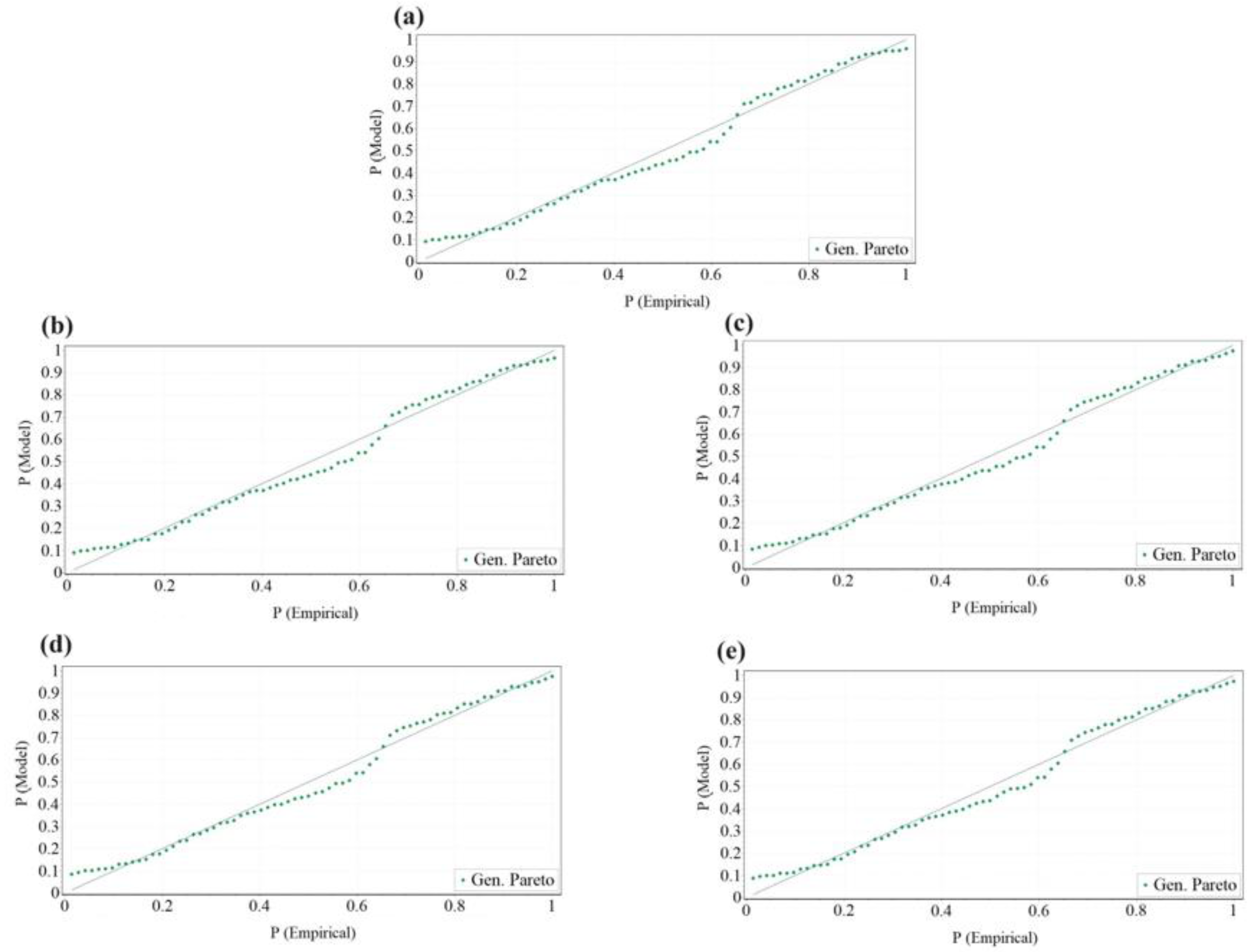
5. Proposing Probability Models

5.1. X-Joints with Retrofitting Plates under Ambient Conditions

Under Laboratory Testing Conditions (20 °C)

Based on the comparative analysis of the various joints, including K–S, A–D, and C–S assessments (refer to Table 8, Table 13 and Table 18), it is evident that the Generalized Petro model demonstrates superior performance in predicting the resistance of X-joints with retrofitting under tensile loading. The findings of the suggested model are presented in

Table 23. Best-fitted distributions for the databases according to the findings of the K-S, A-D, and C-S tests.

		K-S Trial			A-D Trial				C-S Trial
		Distribution	Statistic	Disagreement	Distribution	Statistic	Disagreement	Distribution	Statistic	Disagreement
Database 1	Best	Generalized Pareto	0.09085	0.00%	Gen. Pareto	0.8553	0.00%	Gen. Pareto	3.9917	0.00%
	Suggested	Gen. Pareto	0.09085		Gen. Pareto	0.8553		Gen. Pareto	3.9917
Database 2	Best	Generalized Pareto	0.09008	0.00%	Gen. Pareto	0.82676	0.00%	Gen. Pareto	4.136	0.00%
	Suggested	Gen. Pareto	0.09008		Gen. Pareto	0.82676		Gen. Pareto	4.136
Database 3	Best	Generalized Pareto	0.08382	0.00%	Gen. Pareto	0.75897	0.00%	Gen. Pareto	4.5525	0.00%
	Suggested	Gen. Pareto	0.08382		Gen. Pareto	0.75897		Gen. Pareto	4.5525
Database 4	Best	Generalized Pareto	0.08512	0.00%	Gen. Pareto	0.77009	0.00%	Gen. Pareto	4.5739	0.00%
	Suggested	Generalized Pareto	0.08512		Gen. Pareto	0.77009		Gen. Pareto	4.5739
Database 5	Best	Generalized Pareto	0.08673	0.00%	Gen. Pareto	0.75742	0.00%	Gen. Pareto	6.3724	0.00%
	Suggested	Gen. Pareto	0.08673		Gen. Pareto	0.75742		Gen. Pareto	6.3724

.

The mathematical expressions for the Generalized Pareto distribution are defined through its PDF and CDF as detailed below:

$$f(x)=\left\{\begin{array}{l}\frac{1}{\sigma }{(1+k\frac{(x-\mu )}{\sigma })}^{-(\frac{1}{k}+1)}\hspace{0.17em}\hspace{0.17em}\hspace{0.17em}\hspace{0.17em}\hspace{0.17em}\hspace{0.17em}\hspace{0.17em}\hspace{0.17em}\hspace{0.17em}k\ne 0\\ \frac{1}{\sigma }\exp (\frac{(\mu -x)}{\sigma })\hspace{0.17em}\hspace{0.17em}\hspace{0.17em}\hspace{0.17em}\hspace{0.17em}\hspace{0.17em}\hspace{0.17em}\hspace{0.17em}\hspace{0.17em}\hspace{0.17em}\hspace{0.17em}\hspace{0.17em}\hspace{0.17em}\hspace{0.17em}\hspace{0.17em}\hspace{0.17em}\hspace{0.17em}k=0\end{array}\right.\hspace{0.17em}\hspace{0.17em}\hspace{0.17em}\hspace{0.17em}\hspace{0.17em}\hspace{0.17em}\hspace{0.17em}$$

(19)

$$F(x)=\left\{\begin{array}{l}1-{(1+k\frac{(x-\mu )}{\sigma })}^{-\frac{1}{k}}\hspace{0.17em}\hspace{0.17em}\hspace{0.17em}\hspace{0.17em}\hspace{0.17em}\hspace{0.17em}\hspace{0.17em}\hspace{0.17em}\hspace{0.17em}k\ne 0\\ 1-\exp (\frac{(\mu -x)}{\sigma })\hspace{0.17em}\hspace{0.17em}\hspace{0.17em}\hspace{0.17em}\hspace{0.17em}\hspace{0.17em}\hspace{0.17em}\hspace{0.17em}\hspace{0.17em}\hspace{0.17em}\hspace{0.17em}\hspace{0.17em}\hspace{0.17em}\hspace{0.17em}\hspace{0.17em}k=0\end{array}\right.\hspace{0.17em}\hspace{0.17em}$$

(20)

where k, σ, μ are the shape parameter, scale parameter, and continuous location parameter, in that order. Regarding the maximum load-bearing capacity under normal temperature conditions (as per database 1), this is detailed in Table 7: μ = 205.87, σ = 996.03, and k = −0.16423. As a result, Equations (21) and (22) can be proposed. Within these equations, x represents the resistance value (unit: kN).

$$f(x)=\frac{1}{996.03}{(1-0.16\frac{(x-205.87)}{996.03})}^{(\frac{1}{0.16}-1)}\hspace{0.17em}\hspace{0.17em}$$

(21)

$$F(x)=1-{(1-0.16\frac{(x-205.87)}{996.03})}^{\frac{1}{0.16}}\hspace{0.17em}$$

(22)

In Figure 11a, the theoretical PDF (Equation (21)) and the empirical PDF are presented. Furthermore, in Figure 12a, the proposed CDF (Equation (22)) and the empirical CDF are illustrated. Figure 13a reveals the disagreement for the strengthened joints under laboratory testing conditions (20 °C). Figure 11a, Figure 12a and Figure 13a present that the accuracy of the suggested distribution is good.

5.2. X-Joints with Retrofitting Plates under Tensile Loading and Fire Conditions

5.2.1. At 200 °C

In light of the results from the assessments (referenced in Table 9, Table 14 and Table 19), it has been determined that the Generalized Petro framework is the most effective for predicting the performance of strengthened X-joints under tension at 200 °C. As detailed in Table 7, k = −0.14797, σ = 941.78, and μ = 183.72. Therefore, Equations (23) and (24) serve as the basis for suggesting the PDF and CDF.

$$f(x)=\frac{1}{941.78}{(1-0.15\frac{(x-183.72)}{941.78})}^{(\frac{1}{0.15}-1)}\hspace{0.17em}$$

(23)

$$F(x)=1-{(1-0.15\frac{(x-183.72)}{941.78})}^{\frac{1}{0.15}}$$

(24)

From Figure 11b, Figure 12b and Figure 13b, it can be concluded that the accuracy of the derived distribution for the X-joints with retrofitting plates in brace tension at 200 °C (Equations (23) and (24)) is enough and good.

5.2.2. At 400 °C

Drawing from the results of the three evaluations (presented in Table 10, Table 15 and Table 20), it was determined that the Generalized Petro model outperforms the others. Regarding database 3, as per the information in Table 7, k = −0.11475, σ = 825.93, and μ = 139.06. Consequently, the PDF and CDF can be suggested based on Equations (25) and (26).

$$f(x)=\frac{1}{825.93}{(1-0.12\frac{(x-139.06)}{825.93})}^{(\frac{1}{0.12}-1)}\hspace{0.17em}$$

(25)

$$F(x)=1-{(1-0.12\frac{(x-139.06)}{825.93})}^{\frac{1}{0.12}}\hspace{0.17em}$$

(26)

In Figure 11c, the proposed PDF (Equation (25)) is contrasted to the empirical PDF. Additionally, Figure 12c showcases a comparison between the CDF defined by Equation (26) and its empirical counterpart. The deviation for joints strengthened to withstand fire conditions is highlighted in Figure 13c. The presentations in Figure 11c, Figure 12c and Figure 13c collectively affirm the reliability of the developed model.

5.2.3. At 600 °C

As indicated by the data in Table 11, Table 16 and Table 21, the Generalized Petro model emerges as the superior choice. Pertaining to database 4, the details outlined in Table 7 reveal: μ = 62.824, σ = 381.54, and k = −0.11179. As a result, the PDF and CDF can be suggested based on Equations (27) and (28).

$$f(x)=\frac{1}{381.54}{(1-0.11\frac{(x-62.82)}{381.54})}^{(\frac{1}{0.11}-1)}\hspace{0.17em}$$

(27)

$$F(x)=1-{(1-0.11\frac{(x-62.82)}{381.54})}^{\frac{1}{0.11}}\hspace{0.17em}$$

(28)

Figure 11d and Figure 12d reveal the PDF and CDF of the suggested model and the empirical data for the retrofitted joints under tension at 600 °C, sequentially. Additionally, Figure 13d reveals the disagreement for the strengthened joints under fire conditions. From Figure 11d, Figure 12d and Figure 13d, it can be seen that the suggested PDF and CDF (Equations (27) and (28)) can lead to accurate findings.

5.2.4. At 800 °C

Following the analysis from the C-S, A-D, and K-S tests, as outlined in Table 12, Table 17 and Table 22, it is concluded that the Generalized Petro model stands out as the most effective. For database 5, from Table 7, μ = 16.143, σ = 93.746, and k = −0.12502. As a result, the PDF and CDF can be suggested based on Equations (29) and (30).

$$f(x)=\frac{1}{93.75}{(1-0.13\frac{(x-16.14)}{93.75})}^{(\frac{1}{0.13}-1)}\hspace{0.17em}$$

(29)

$$F(x)=1-{(1-0.13\frac{(x-16.14)}{93.75})}^{\frac{1}{0.13}}$$

(30)

Figure 11e exhibits the PDF of the Generalized Petro distribution (Equation (29)) and the associated empirical PDF. Furthermore, Figure 12e presents the CDF of the proposed model (Equation (30)) and the empirical CDF. Figure 13e reveals the disagreement for the strengthened joints under fire conditions. Figure 11e, Figure 12e and Figure 13e present that the suggested distribution (Equations (29) and (30)) can accurately estimate the behavior.

6. Conclusions

The study developed a theoretical framework for predicting the distribution of ultimate resistance in CHS X-joints strengthened with retrofitting plates, subjected to axial tensile loads in both ambient and various fire scenarios, utilizing 360 finite element models (FEMs). The significant contributions of this research include:

• Utilizing the Kolmogorov–Smirnov, Anderson–Darling, and Chi-squared analyses on five different datasets underscored the superiority of the Generalized Petro distribution in gauging the strength of X-joints fortified with retrofitting plates under tension, maintaining this distinction across a range of temperature scenarios.
• The introduction of five theoretical PDFs and CDFs offers a nuanced understanding of the ultimate resistance behaviors of X-joints under the specified conditions, facilitating precise engineering and design strategies.
• The characteristics of the recommended theoretical PDF and CDF are precisely defined by the location parameter (μ = 205.87), scale parameter (δ = 996.03), and shape parameter (k = −0.16423) capturing the essence of the structural performance under laboratory testing conditions (20 °C).
• Within the suggested PDF and CDF for joints strengthened to withstand the ambient conditions, the parameters are meticulously defined as follows: the scale parameter (δ) is set at 996.03, the continuous location parameter (μ) is set at 205.87, and the shape parameter (k) is set at −0.16423.
• For the proposed theoretical PDF and CDF tailored to joints at 200 °C, the parameters μ, δ, and k are set as 183.72, 941.78, and −0.14797, sequentially. At 400 °C, these parameters are adjusted to 139.06, 825.93, and −0.11475, in that order.
• At 600 °C, the μ, δ, and k are 62.824, 381.54, and −0.11179, sequentially. At 800 °C, the μ, δ, and k are 16.143, 93.746, and −0.12502, sequentially.
• Ultimately, the alignment of the proposed theoretical values with observed data indicates a strong correlation between the suggested theoretical PDFs and CDFs and the FE Model data.

References

1. Xu, J.; Yang, L.; Han, J.; Han, Z.; Tu, J.; Li, Z. Fire resistance behavior of earthquake-damaged tubular T-joints at elevated temperatures. J. Constr. Steel Res. 2019, 159, 176–188. [Google Scholar] [CrossRef]
2. Ahmadi, H. Probabilistic analysis of the DoB in axially-loaded tubular KT-joints of offshore structures. Appl. Ocean Res. 2019, 87, 64–80. [Google Scholar] [CrossRef]
3. Nassiraei, H.; Zhu, L.; Lotfollahi-Yaghin, M.A.; Ahmadi, H. Static capacity of tubular X-joints reinforced with collar plate subjected to brace compression. Thin-Walled Struct. 2017, 119, 256–265. [Google Scholar] [CrossRef]
4. Shao, Y.-B. Static strength of collar-plate reinforced tubular T-joints under axial loading. Steel Compos. Struct. 2016, 21, 323–342. [Google Scholar] [CrossRef]
5. Choo, Y.S.; Liang, J.X.; Van der Vegte, G.J.; Liew, J.Y.R. Static strength of collar plate reinforced CHS X-joints loaded by in-plane bending. J. Constr. Steel Res. 2004, 60, 1745–1760. [Google Scholar] [CrossRef]
6. Choo, Y.S.; Liang, J.X.; Van der Vegte, G.J.; Zettlemoyer, N.; Li, B.H.; Liew, J.Y.R. Static strength of T-joints reinforced with doubler or collar plates. I: Experimental investigations. J. Struct. Eng. 2005, 31, 119–128. [Google Scholar] [CrossRef]
7. Van der Vegte, G.J.; Choo, Y.S.; Liang, J.X.; Zettlemoyer, N.; Liew, G.J.R. Static strength of T-joints reinforced with doubler or collar plates, II: Numerical simulations. J. Struct. Eng. 2005, 131, 129–138. [Google Scholar] [CrossRef]
8. Gao, F.; Guan, X.Q.; Zhu, H.P.; Liu, X.N. Fire resistance behaviour of tubular T-joints reinforced with collar plates. J. Constr. Steel Res. 2015, 115, 106–120. [Google Scholar] [CrossRef]
9. Tan, K.H.; Fung, T.C.; Nguyen, M.P. Structural behavior of CHS T-Joints subjected to brace axial compression in fire conditions. J. Struct. Eng. 2013, 139, 73–84. [Google Scholar] [CrossRef]
10. Ozyurt, E.; Wang, Y.C.; Tan, K.H. Elevated temperature resistance of welded tubular joints under axial load in the brace member. Eng. Struct. 2013, 59, 574–586. [Google Scholar] [CrossRef]
11. Ozyurt, E.; Wang, Y.C. A numerical investigation of static resistance of welded planar steel tubular joints under in-plane and out-of-plane bending at elevated temperatures. Eng. Struct. 2019, 199, 109622. [Google Scholar] [CrossRef]
12. Azari-Dodaran, N.; Ahmadi, H. Structural behavior of right-angle two-planar tubular TT-joints subjected to axial loadings at fire-induced elevated temperatures. Fire Saf. J. 2019, 108, 102849. [Google Scholar] [CrossRef]
13. Pandey, M.; Young, B. Cold-formed high strength steel CHS-to-RHS T- and X-joints: Performance and design after fire exposures. Thin-Walled Struct. 2023, 189, 110793. [Google Scholar] [CrossRef]
14. Nassiraei, H. Probability distribution models for the ultimate strength of tubular T/Y-joints reinforced with collar plates at room and different fire conditions. Ocean Eng. 2023, 270, 113557. [Google Scholar] [CrossRef]
15. Zhao, Z.; Liu, H.; Liang, B. Probability distribution of the compression capacity of welded hollow spherical joints with randomly located corrosion. Thin-Walled Struct. 2019, 137, 167–176. [Google Scholar] [CrossRef]
16. Chen, M.T.; Chen, Y.; Young, B. Experimental investigation on cold-formed steel elliptical hollow section T-joints. Eng. Struct. 2023, 283, 115593. [Google Scholar] [CrossRef]
17. Chen, M.T.; Pandey, M.; Young, B. Mechanical properties of cold-formed steel semi-oval hollow sections after exposure to ISO-834 fire. Thin-Walled Struct. 2021, 167, 108202. [Google Scholar] [CrossRef]
18. Chen, M.T.; Chen, Y.; Young, B. Static strengths of cold-formed steel elliptical hollow section X-joints. Thin-Walled Struct. 2023, 191, 110997. [Google Scholar] [CrossRef]
19. Pandey, M.; Young, B. Design of cold-formed high strength steel rectangular hollow section T-joints under post-fire conditions. J. Constr. Steel Res. 2023, 208, 107941. [Google Scholar] [CrossRef]
20. Ozyurt, E.; Wang, Y.C. Resistance of axially loaded T-and X-joints of elliptical hollow sections at elevated temperatures–A finite element study. Structures 2018, 14, 15–31. [Google Scholar] [CrossRef]
21. Xu, Y.; Zhang, M.; Zheng, B. Design of cold-formed stainless steel circular hollow section columns using machine learning methods. Structures 2021, 33, 2755–2770. [Google Scholar] [CrossRef]
22. Oeng, P.; Chen, M.T.; Young, B. Cold-formed steel T-joints with semi-oval hollow section chord: Experimental insight and finite element modelling. ce/papers 2023, 6, 1562–1567. [Google Scholar] [CrossRef]
23. Huang, S.; Deng, X.; Wang, Y. Experimental investigations of optimized 3D Printing Planar X-joints manufactured by stainless steel and high-strength steel. Eng. Struct. 2023, 285, 116054. [Google Scholar] [CrossRef]
24. Huang, S.; Deng, X.; Lam, L.K. Integrated design framework of 3D printed planar stainless tubular joint: Modelling, optimization, manufacturing, and experiment. Thin-Walled Struct. 2021, 169, 108463. [Google Scholar] [CrossRef]
25. Zuo, W.; Chen, M.T.; Chen, Y.; Zhao, O.; Cheng, B.; Zhao, J. Additive manufacturing oriented parametric topology optimization design and numerical analysis of steel joints in gridshell structures. Thin-Walled Struct. 2023, 188, 110817. [Google Scholar] [CrossRef]
26. Meng, X.; Zhi, J.; Xu, F.; Gardner, L. Novel hybrid sleeve connections between 3D printed and conventional tubular steel elements. Eng. Struct. 2024, 302, 117269. [Google Scholar] [CrossRef]
27. Fung, T.; Soh, C.; Gho, W.; Qin, F. Ultimate capacity of completely overlapped tubular joints. J. Constr. Steel Res. 2001, 57, 855–880. [Google Scholar] [CrossRef]
28. Nassiraei, H. Local joint flexibility of CHS X-joints reinforced with collar plates in jacket structures subjected to axial load. Appl. Ocean Res. 2019, 93, 101961. [Google Scholar] [CrossRef]
29. American Welding Society (AWS). Structural Welding Code: AWS D 1.1.; American Welding Society (AWS): Miami, FL, USA, 2015. [Google Scholar]
30. EN 1993-1-2; CEN, Design of Steel Structures. Part: EN 1993-1-2-Structural FIre Design. British Standard Institute: London, UK, 2005.
31. Lesani, M.; Bahaari, M.R.; Shokrieh, M.M. Detail investigation on un-stiffened T/Y tubular joints behavior under axial compressive loads. J. Constr. Steel Res. 2012, 80, 91–99. [Google Scholar] [CrossRef]
32. Ding, Y.; Zhu, L.; Zhang, K.; Bai, Y.; Sun, H. CHS X-joints strengthened by external stiffeners under brace axial tension. Eng. Struct. 2018, 171, 445–452. [Google Scholar] [CrossRef]
33. Kottegoda, N.T.; Rosso, R. Applied Statistics for Civil and Environmental Engineers, 2nd ed.; Blackwell Publishing Ltd.: Oxford, UK, 2008. [Google Scholar]
34. Stephens, M.A. EDF Statistics for Goodness of Fit and Some Comparisons. J. Am. Stat. Assoc. 1974, 69, 730–737. [Google Scholar] [CrossRef]
35. Hu, S.; Wang, W.; Lin, X. Two-stage machine learning framework for developing probabilistic strength prediction models of structural components: An application for RHS-CHS T-joint. Eng. Struct. 2022, 266, 114548. [Google Scholar] [CrossRef]
Figure 1. Geometrical notation for an X-joint with the plates.
Buildings 14 02105 g001
Figure 3. Comparison between the numerical and experimental findings. (ah) shows the load-displacements of the S1–S11 for validation.
Buildings 14 02105 g003
Figure 4. Comparison between the failure modes of the experimental tests [3,6,9,32] and the present FE model (S4, S8, and S11 are not shown).
Buildings 14 02105 g004
Figure 5. Deformed X-joints at 600 °C under tension.
Buildings 14 02105 g005
Figure 8. Probability density functions shaped to the histograms produced for the ultimate resistance of the joints: (a) 20, (b) 200, (c) 400, (d) 600, (e) 800 °C.
Buildings 14 02105 g008
Figure 9. Theoretical continuous CDFs fitted to the empirical distribution functions of produced samples: (a) 20, (b) 200, (c) 400, (d) 600, (e) 800 °C.
Buildings 14 02105 g009
Figure 10. The comparison between the theoretical and empirical values: (a) 20, (b) 200, (c) 400, (d) 600, (e) 800 °C.
Buildings 14 02105 g010
Figure 11. Suggested theoretical PDF shaped to the histograms produced for the ultimate resistance of the strengthened joints: (a) 20, (b) 200, (c) 400, (d) 600, (e) 800 °C.
Buildings 14 02105 g011
Figure 12. Suggested theoretical CDF fitted to the empirical distribution functions of produced samples: (a) 20, (b) 200, (c) 400, (d) 600, (e) 800 °C.
Buildings 14 02105 g012
Figure 13. The comparison between the suggested theoretical and empirical values: (a) 20, (b) 200, (c) 400, (d) 600, (e) 800 °C.
Buildings 14 02105 g013