
Multi-Objective Optimization in Construction Project Management Based on NSGA-III: Pareto Front Development and Decision-Making


Abstract
:1. Introduction
1.1. Research Background
1.2. Literature Review
1.2.1. Research on Objective Dimensionality
1.2.2. Research on Objective Model Construction
1.2.3. Research on Algorithms
1.2.4. Research on Decision-Making Processes
2. Research Methods
2.1. MOP Theory
2.2. Model Establishment
2.2.1. Basic Assumptions
2.2.2. Establishment of Time Model
2.2.3. Establishment of Cost Model
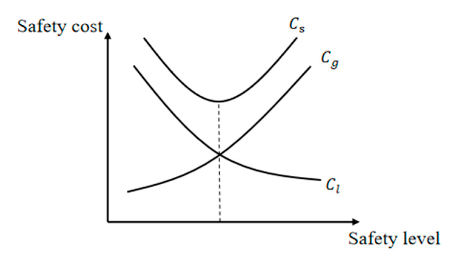
2.2.4. Establishment of Safety Model
2.2.5. Establishment of Carbon Emissions Model
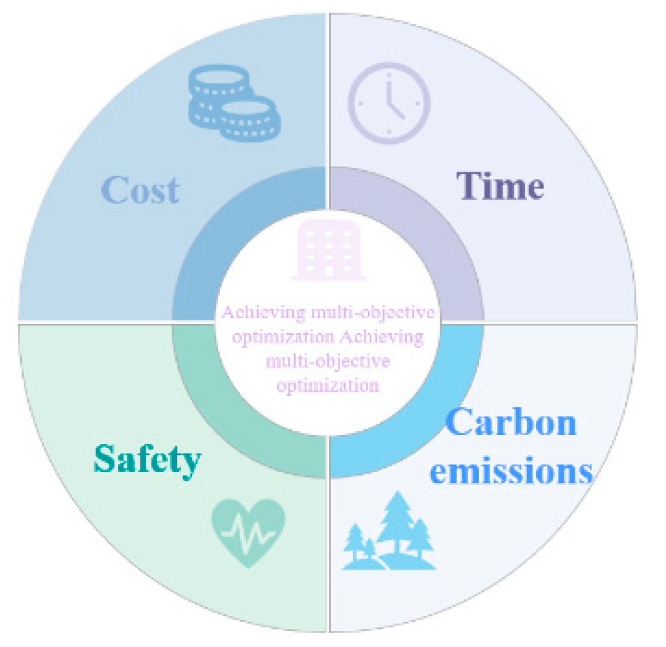
2.2.6. Time-Cost–Safety–Carbon Emissions Integrated Optimization Model
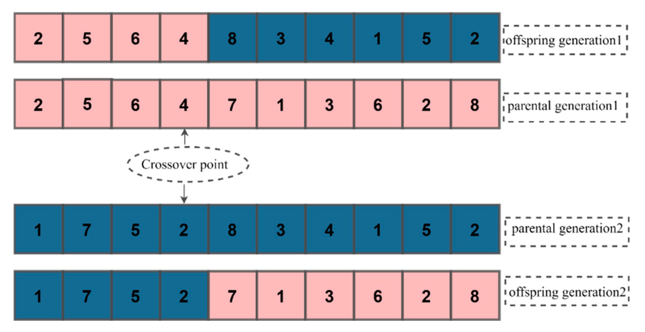
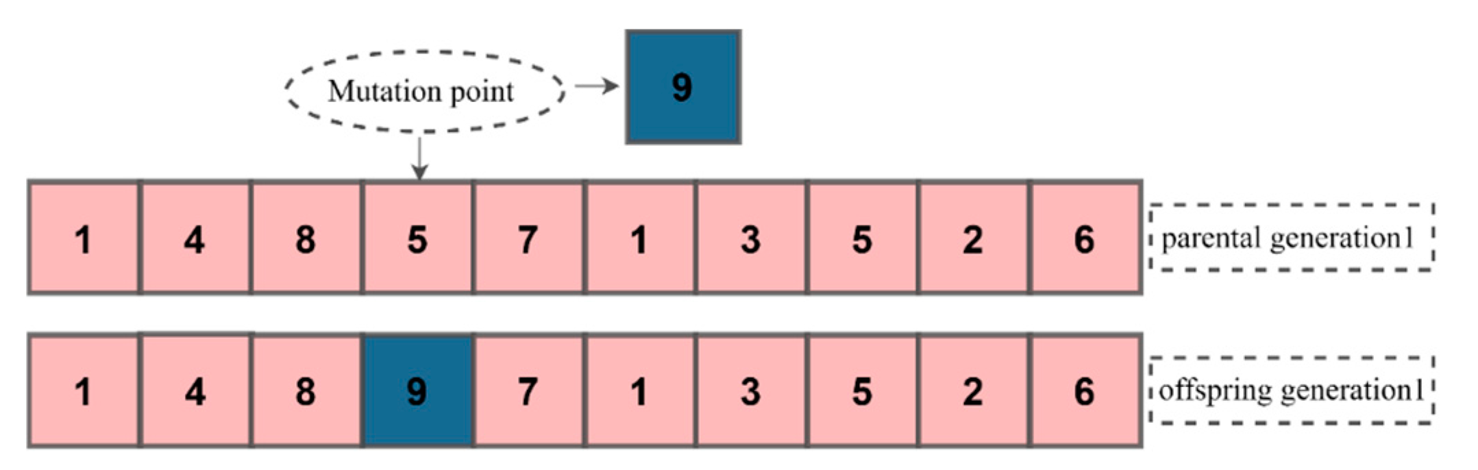
2.3. Algorithm Design
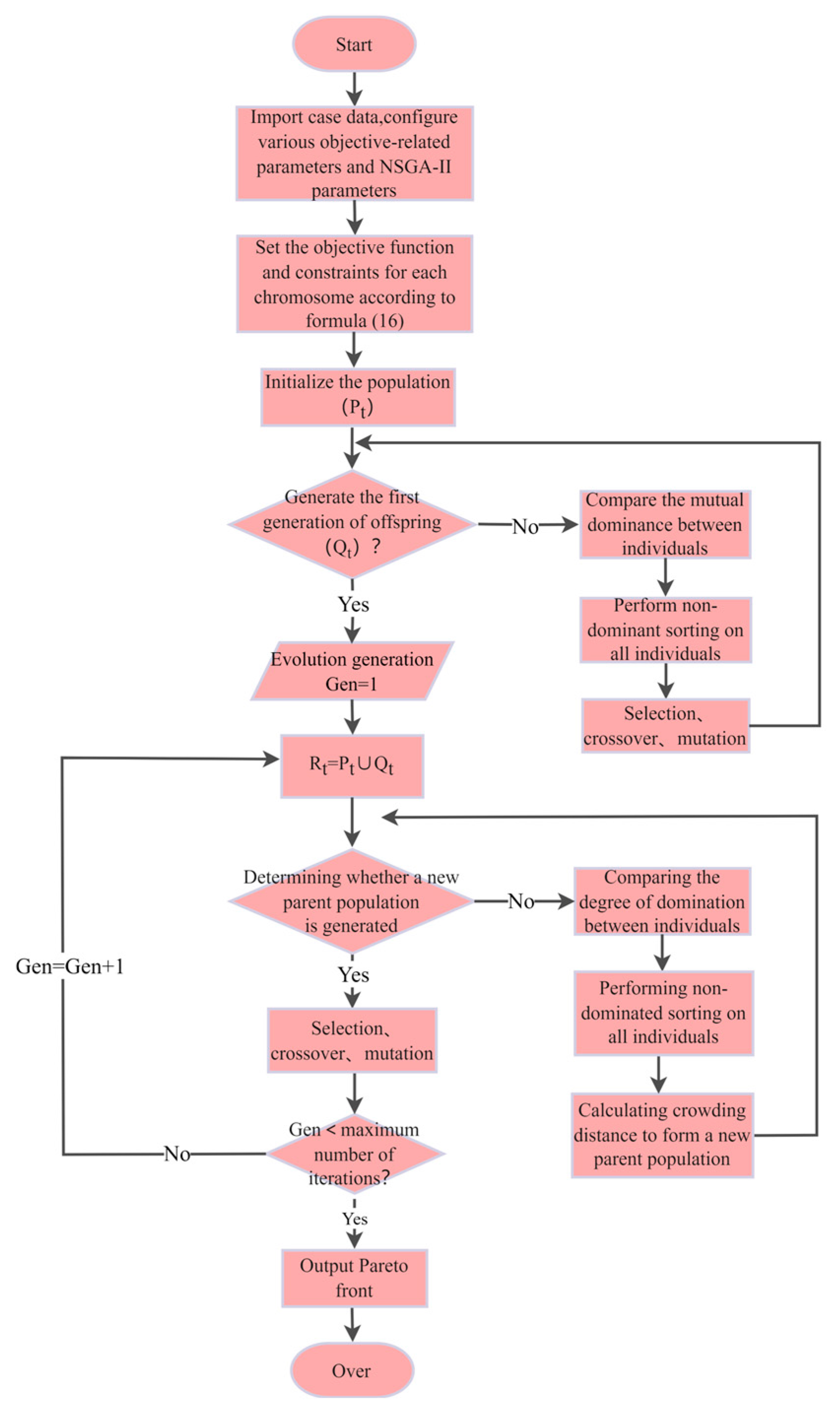
2.3.1. NSGA-II
2.3.2. NSGA-III
2.4. Decision Method
2.4.1. Entropy Method
2.4.2. VIKOR Method
3. Case Study
3.1. Case Overview
3.2. Data Processing
4. Model Result
4.1. Parameter Setting
4.1.1. NSGA-II Solution Results
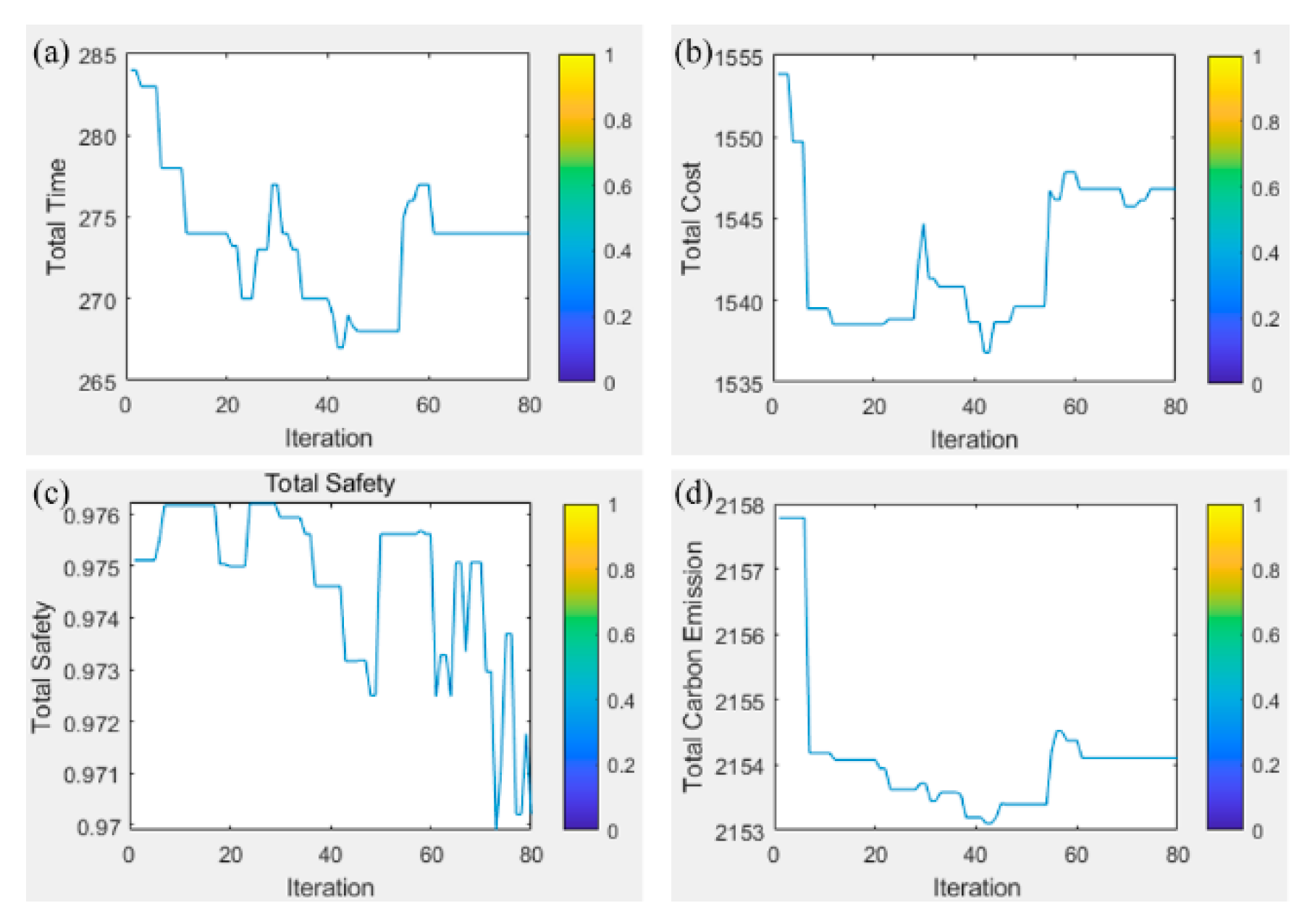
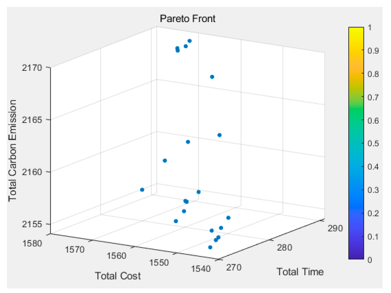
4.1.2. NSGA-III Solution Results
4.2. Solution Choosing
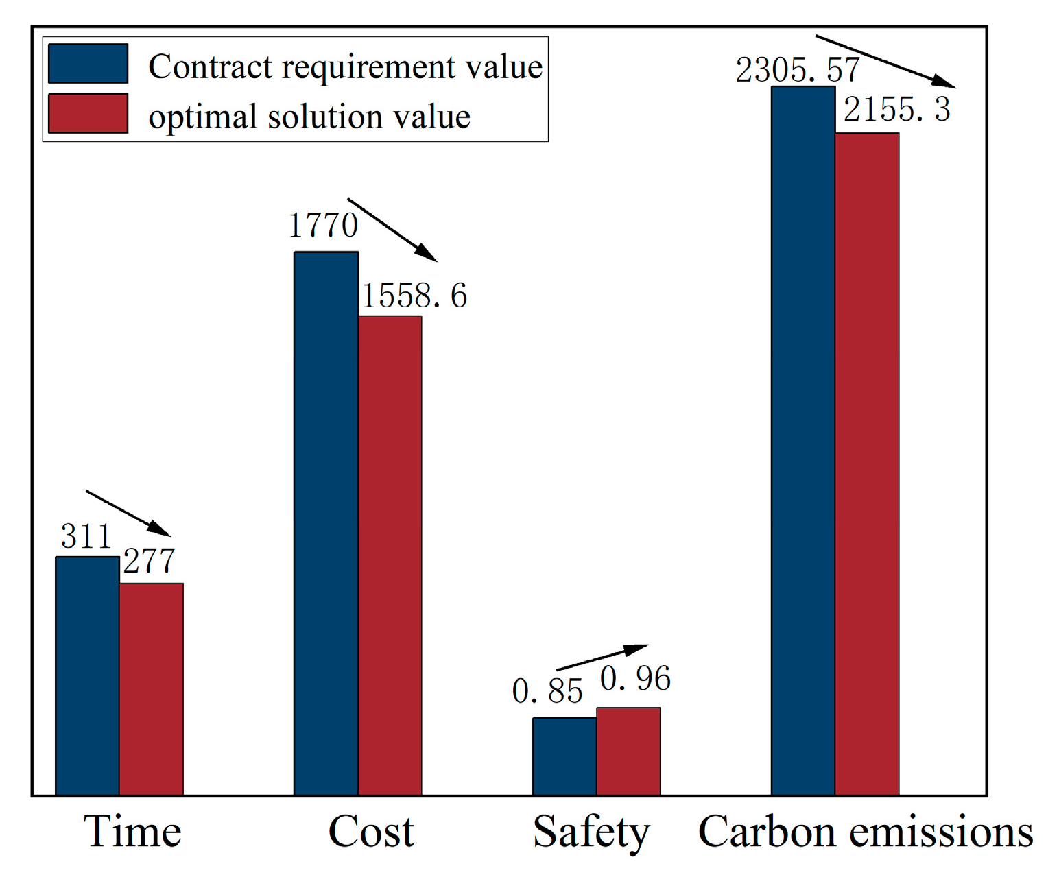
4.3. Result Analysis
5. Discussion
6. Conclusions
Author Contributions
Funding
Data Availability Statement
Conflicts of Interest
References
- “14th Five-Year” Plan for Energy Conservation and Green Building Development. Build. Superv. Insp. Cost 2022, 15, 1–9.
- Kim, K.; Walewski, J.; Cho, Y.K. Multiobjective Construction Schedule Optimization Using Modified Niched Pareto Genetic Algorithm. J. Manag. Eng. 2016, 32, 04015038. [Google Scholar] [CrossRef]
- Xiang, Y.; Ma, Y.; Wei, Y. Comprehensive Objective Optimization Analysis of Construction Projects under Multiobjective Particle Swarm Optimization. Mob. Inf. Syst. 2022, 2022, 3670074. [Google Scholar] [CrossRef]
- He, W.; Shi, Y. Multiobjective construction optimization model based on quantum genetic algorithm. Adv. Civ. Eng. 2019, 2019, 1–8. [Google Scholar] [CrossRef]
- Xiong, Y.; Kuang, Y.P. Optimization of Construction Project Schedule and Cost Based on Ant Colony Algorithm. Syst. Eng. Theory Pract. 2007, 27, 7. [Google Scholar] [CrossRef]
- Babu, A.J.G.; Suresh, N. Project management with time, cost, and quality considerations. Eur. J. Oper. Res. 1996, 88, 320–327. [Google Scholar] [CrossRef]
- Pollack-Johnson, B.; Liberatore, M.J. Incorporating Quality Considerations Into Project Time/Cost Tradeoff Analysis and Decision Making. IEEE Trans. Eng. Manag. 2006, 53, 534–542. [Google Scholar] [CrossRef]
- Heravi, G.; Faeghi, S. Group Decision Making for Stochastic Optimization of Time, Cost, and Quality in Construction Projects. J. Comput. Civ. Eng. 2014, 28, 275–283. [Google Scholar] [CrossRef]
- Wang, J.; Wang, Z.; Liu, H. Multi-objective Stochastic Time-cost-quality Optimization for Construction Projects Based on the Reliability Theory. KSCE J. Civ. Eng. 2023, 27, 4545–4556. [Google Scholar] [CrossRef]
- Song, Y. Green Construction Multi-objective Management Equilibrium Optimization of Construction Engineering Projects Based on Genetic Algorithm. Autom. Technol. Appl. 2023, 42, 165–169. [Google Scholar]
- Keshavarz, E.; Shoul, A. Project Time-Cost-Quality Trade-off Problem: A Novel Approach Based on Fuzzy Decision Making. Int. J. Uncertain. Fuzziness Knowl.-Based Syst. 2020, 28, 545–567. [Google Scholar] [CrossRef]
- Hussein, M.; Darko, A.; Eltoukhy, A.E.; Zayed, T. Sustainable logistics planning in modular integrated construction using multimethod simulation and Taguchi approach. J. Constr. Eng. Manag. 2022, 148, 04022022. [Google Scholar] [CrossRef]
- Liu, X.F.; Chen, T.; Wu, S.Y. Research on Multi-objective Collaborative Optimization of Engineering Projects. Chin. Eng. Sci. 2010, 12, 90–94. [Google Scholar]
- Mateo, J.R.S.C. An Integer Linear Programming Model Including Time, Cost, Quality, and Safety. IEEE Access 2019, 7, 168307–168315. [Google Scholar] [CrossRef]
- Hao, F.F. Research on Multi-Objective Optimization of Engineering Projects with Safety Factors; Xi’an University of Technology: Xi’an, China, 2019. [Google Scholar]
- Jin, C. Research on Multi-Objective Optimization of Construction Management for Expressway Engineering Projects: A Case Study of JX Expressway; School of Engineering Cost and Investment Management, Hebei GEO University: Shijiazhuang, China, 2022. [Google Scholar]
- Zareei, M.; Hassan-Pour, H.A. A multi-objective resource-constrained optimization of time-cost trade-off problems in scheduling project. Iran. J. Manag. Stud. 2015, 8, 653. [Google Scholar]
- Shahriari, M. Multi-objective optimization of discrete time–cost tradeoff problem in project networks using non-dominated sorting genetic algorithm. J. Ind. Eng. Int. 2016, 12, 159–169. [Google Scholar] [CrossRef]
- Liu, X. Research on Dynamic Optimization Layout of Construction Project Facilities Based on NSGA-II Algorithm; Chongqing University: Chongqing, China, 2018. [Google Scholar]
- Wang, X.; Cui, F.; Cui, L.; Jiang, D. Research on a Multi-Objective Optimization Design for the Durability of High-Performance Fiber-Reinforced Concrete Based on a Hybrid Algorithm. Coatings 2023, 13, 2054. [Google Scholar] [CrossRef]
- Hussein, M.; Eltoukhy, A.E.; Darko, A.; Eltawil, A. Simulation-Optimization for the Planning of Off-Site Construction Projects: A Comparative Study of Recent Swarm Intelligence Metaheuristics. Sustainability 2021, 13, 13551. [Google Scholar] [CrossRef]
- Tegos, N.; Papadopoulos, I.; Aretoulis, G. Definition of Compliance Criterion Weights for Bridge Construction Method Selection and Their Application in Real Projects. Buildings 2023, 13, 2891. [Google Scholar] [CrossRef]
- Qiu, X.Y. Research on Multi-Objective Optimization of Engineering Projects Based on Quantum Particle Swarm Optimization Algorithm; School of Management Science and Engineering, Hebei University of Engineering: Handan, China, 2019. [Google Scholar]
- Wu, W.; Guo, J.; Li, J.; Hou, H.; Meng, Q.; Wang, W. A multi-objective optimization design method in zero energy building study: A case study concerning small mass buildings in cold district of China. Energy Build. 2018, 158, 1613–1624. [Google Scholar] [CrossRef]
- Rahimbakhsh, H.; Kohansal, M.E.; Tarkashvand, A.; Faizi, M.; Rahbar, M. Multi-objective optimization of natural surveillance and privacy in early design stages utilizing NSGA-II. Autom. Constr. 2022, 143, 104547. [Google Scholar] [CrossRef]
- Chen, Y.M. Research on Multi-Objective Equilibrium Optimization of Green Construction Projects Based on GA-PSO Algorithm; Yangzhou University: Yangzhou, China, 2019. [Google Scholar]
- Mitropoulos, P.T. The role of production and teamwork practices in construction safety: A cognitive model and an empirical case study. J. Saf. Res. 2009, 40, 265–275. [Google Scholar] [CrossRef] [PubMed]
- Kolahan, F.; Golmezerji, R.; Moghaddam, M.A. Multi Objective Optimization of Turning Process Using Grey Relational Analysis and Simulated Annealing Algorithm. Appl. Mech. Mater. 2011, 110–116, 2926–2932. [Google Scholar] [CrossRef]
- Lee, D.; Lee, C.; Guk, H. Multi-objective Optimization System for Time-Cost-Environment-Quality Trade-off in Construction Project. J. Archit. Inst. Korea Struct. Constr. 2015, 31, 79–88. [Google Scholar]
- Li, Y.; Wang, S.; He, Y. Multi-objective Optimization of Construction Project Based on Improved Ant Colony Algorithm. Teh. Vjesn.-Tech. Gaz. 2020, 27, 184–190. [Google Scholar]
- He, L.L. Research on Multi-objective Optimization of Green Construction Projects Based on Improved NSGA-II Algorithm; Guizhou University: Guiyang, China, 2022. [Google Scholar]
- “14th Five-Year”Construction Industry Development Plan. Cost Eng. Manag. 2022, 4–10.
- Xi, Y.G.; Chai, T.Y.; Yun, W.M. A Survey of Genetic Algorithms. Control. Theory Appl. 1996, 13, 697–708. [Google Scholar]
- Deb, K.; Pratap, A.; Agarwal, S.; Meyarivan, T.A.M.T. A fast and elitist multiobjective genetic algorithm: NSGA-II. IEEE Trans. Evol.Comput. 2002, 6, 182–197. [Google Scholar] [CrossRef]
- Deb, K.; Jain, H. An Evolutionary Many-Objective Optimization Algorithm Using Reference-Point-Based Nondominated Sorting Approach, Part I: Solving Problems with Box Constraints. IEEE Trans. Evol. Comput. 2014, 18, 577–601. [Google Scholar] [CrossRef]
- Wang, H.Y.; Gao, P.C.; Xie, Y.R.; Song, C.Q.; Wang, Y.H. Land Use Optimization Based on Genetic Algorithms: A Comparative Study of NSGA-II and NSGA-III. Acta Ecol. Sin. 2023, 43, 639–649. [Google Scholar]
- Zhang, J.; Wang, S.; Tang, Q.; Zhou, Y.; Zeng, T. An improved NSGA-III integrating adaptive elimination strategy to solution of many-objective optimal power flow problems. Energy 2019, 172, 945–957. [Google Scholar] [CrossRef]
- Shemshadi, A.; Shirazi, H.; Toreihi, M.; Tarokh, M.J. A fuzzy VIKOR method for supplier selection based on entropy measure for objective weighting. Expert Syst. Appl. 2011, 38, 12160–12167. [Google Scholar] [CrossRef]
- Chu, X.H. Research on Performance Evaluation of State-Owned Construction Enterprises Based on Entropy Method; Beijing University of Chemical Technology: Beijing, China, 2023. [Google Scholar]
- Ma, N. Research on Urban Livability Evaluation Based on PCA-Entropy Method Model; Chongqing University: Chongqing, China, 2021. [Google Scholar]
- Jiang, Z.Z.J. Research on Multi-Scenario Flood Risk Assessment Based on Entropy Weighting and GIS; Nanchang University: Nanchang, China, 2020. [Google Scholar]
- Opricovic, S.; Tzeng, G.H. Extended VIKOR method in comparison with outranking methods. Eur. J. Oper. Res. 2007, 178, 514–529. [Google Scholar] [CrossRef]
- Pan, R.S. Multi-Objective Optimization and Decision-Making for Complex Mechanical Product Assembly Based on Improved NSGA-III; Shihezi University: Shihezi, China, 2023. [Google Scholar]
- Pouraminian, M.; Pourbakhshian, S. Multi-criteria shape optimization of open-spandrel concrete arch bridges: Pareto front development and decision-making. World J. Eng. 2019, 16, 670–680. [Google Scholar] [CrossRef]
- Peng, J.; Feng, Y.; Zhang, Q.; Liu, X. Multi-objective Integrated Optimization Study of Prefabricated Building Projects Introducing Sustainable Levels. Sci. Rep. 2023, 13, 2821. [Google Scholar] [CrossRef]
- Wang, R.; Li, M.; Wu, Z.H. Research on Multi-Objective Optimization of Temporary Facilities Layout for Prefabricated Construction Sites Based on SLP and NSGA-II. Constr. Technol. 2024, 53, 125–132. [Google Scholar]
- Yan, T.W. Research on Multi-Objective Optimization of Construction Process for Steel-Concrete Composite Columns Considering Carbon Emissions; Beijing Jiaotong University: Beijing, China, 2023. [Google Scholar]


| Author (Year) | Research Subject/Question | Objectives/KPIS | Algorithm/Key Technique | Whether to Conduct Algorithm Comparison | Whether to Consider Environmental Impact | Whether to Make Decisions | Reference |
|---|---|---|---|---|---|---|---|
| Xiong (2007) | Engineering project | Time—Cost | ACO | No | No | No | [5] |
| Babu (1996) | Engineering project | Time—Cost—Quality | Critical path programming (CPM) | No | No | No | [6] |
| Pollack-Johnson (2006) | Engineering project | Time—Cost—Quality | AHP | No | No | No | [7] |
| Heravi (2014) | Engineering project | Time—Cost—Quality | Monte Carlo method, OWA | No | No | Yes | [8] |
| Wang et al. (2023) | Engineering project | Time—Cost—Quality | PSO | No | No | No | [9] |
| Song (2023) | Engineering project | Time—Cost—Quality—Environment | GA | No | Yes | No | [10] |
| Keshavarz E (2020) | Teaching building | Time—Cost—Quality | fuzzy decision-making approach | No | No | Yes | [11] |
| Hussein M et al. (2022) | Logistics planning | Minimize project time, SC costs and SC emissions | Simulation (ABM and DES), DOE, and optimization | No | Yes | Yes | [12] |
| Liu (2010) | Engineering project | Time—Cost—Quality—Resources | PSO | No | No | No | [13] |
| San Cristobal Mateo J R (2019) | Project planning and scheduling | Time—Cost—Quality—Safety | CPM | No | No | No | [14] |
| Hao (2019) | Reservoir engineering | Time—Cost—Security risk | PSO | No | No | No | [15] |
| Jin (2022) | Highway | Time—Cost—Quality | NSGA-II | Yes | No | No | [16] |
| Zareei (2015) | Project scheduling issues | Time—Cost | NSGA—II, MOSA, MOPSO | Yes | No | No | [17] |
| Shahriari (2016) | Engineering project | Time—Cost | NSGA-II | No | No | No | [18] |
| Liu (2018) | Dynamic layout of construction site facilities | Maximizing the reduction of total facility processing costs and unsafe factors | NSGA-II | No | No | No | [19] |
| Wang (2023) | High-performance fiber-reinforced concrete | Material Ratio–Freeze Resistance–Permeability Resistance–Cost | NSGA-III, response surface methodology | No | No | No | [20] |
| Hussein M (2021) | Construction planning issues (Bridge project) | Finding the optimal planning decision to enhance the sustainability of the built environment | firefly algorithm, grey wolf optimization, the whale optimization algorithm, the salp swarm algorithm, improved bat algorithm | Yes | No | No | [21] |
| Tegos N et al. (2023) | bridge construction methods | Through multi-criteria decision-making, the most appropriate bridge construction method is selected under varying circumstances | Multi-criteria analysis, questionnaire | No | Yes | Yes | [22] |
| Qiu (2019) | Commercial complex | Time—Cost—Quality—Safety | Quantum Particle Swarm Optimization (QPSO), Entropy—TOPSIS method | No | No | Yes | [23] |
| Wu et al. (2018) | Small Mass Buildings in Cold District of China | Cost—Energy | NSGA-II, grey correlation multi-level comprehensive evaluation method | No | No | Yes | [24] |
| Rahimbakhsh H et al. (2022) | Residential complex | Balancing individual privacy and public space within residential buildings to achieve optimal surveillance and privacy conditions | NSGA-II, TOPSIS | No | No | Yes | [25] |
| This Study | Office building construction project | Time—Cost–Safety—Carbon Emissions | NSGA-II, NSGA-III | Yes | Yes | Yes |
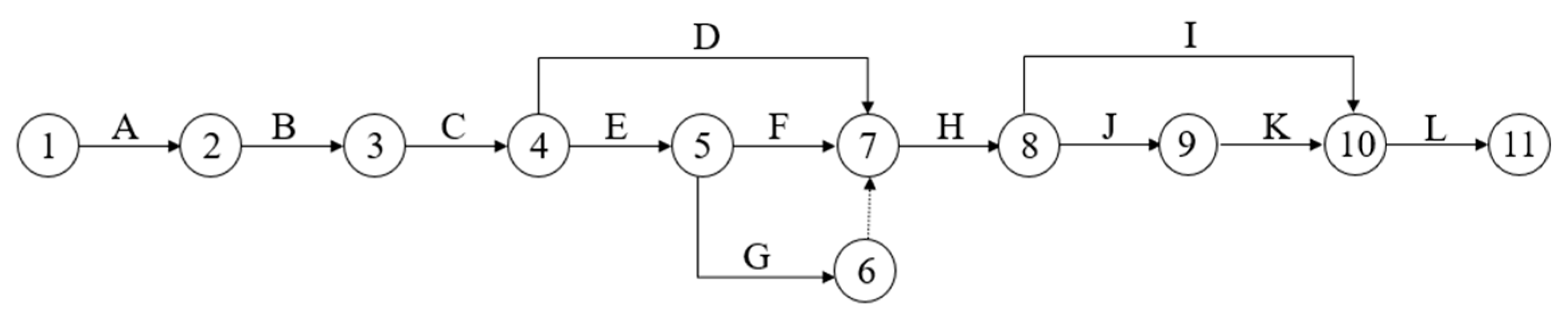
| Process Number | Process Code | Predecessor Task | Successor Task | Process Name |
|---|---|---|---|---|
| 1 | A | - | B | Earthwork excavation |
| 2 | B | A | C | Foundation construction |
| 3 | C | B | D, E | Basement structure and first-floor beam |
| 4 | D | C | H | Basement wall treatment |
| 5 | E | C | F | Main structure construction |
| 6 | F | E | H | Roof construction |
| 7 | G | E | H | Scaffolding removal |
| 8 | H | D, F, G | I | Main structure maintenance and Inspection |
| 9 | I | H | J | Masonry construction |
| 10 | J | H | L | Main roof decoration and treatment |
| 11 | K | J | K | Drainage, roads, and other facilities |
| 12 | L | I, K | - | Completion of cleaning and preparation |
| Process Number | tdij | tij | tcij | Czijmin | Czijmax | Cjijmin | Cjijmax | Ceij | p0ij | Δpminij | Δpmaxij | Eminij | Emaxij |
|---|---|---|---|---|---|---|---|---|---|---|---|---|---|
| A | 20 | 21 | 25 | 34 | 51 | 14 | 17 | 16.51 | 0.15 | 0.05 | 0.90 | 5.5 | 7.8 |
| B | 29 | 32 | 37 | 75 | 88 | 21 | 24 | 13.55 | 0.12 | 0.10 | 0.90 | 407.4 | 425.88 |
| C | 20 | 22 | 23 | 160 | 208 | 14 | 17 | 14.90 | 0.12 | 0.15 | 0.93 | 241.5 | 294 |
| D | 13 | 15 | 22 | 11 | 16 | 11 | 13 | 13.19 | 0.10 | 0.05 | 0.85 | 42.1 | 58 |
| E | 58 | 60 | 69 | 647 | 720 | 42 | 47 | 19.58 | 0.03 | 0.04 | 0.90 | 1144.5 | 1184.6 |
| F | 15 | 18 | 20 | 71 | 81 | 12 | 14 | 10.52 | 0.04 | 0.009 | 0.92 | 6.3 | 10.06 |
| G | 7 | 8 | 11 | 13 | 20 | 5 | 7 | 3.71 | 0.10 | 0.09 | 0.90 | 0.32 | 0.55 |
| H | 27 | 32 | 34 | 40 | 48 | 19 | 21 | 7.25 | 0.08 | 0.10 | 0.90 | 2.4 | 3.4 |
| I | 32 | 35 | 43 | 42 | 54 | 24 | 26 | 10.94 | 0.11 | 0.05 | 0.92 | 299.37 | 316 |
| J | 20 | 21 | 25 | 58 | 70 | 15 | 17 | 7.97 | 0.12 | 0.02 | 0.86 | 2.53 | 3.99 |
| K | 24 | 28 | 33 | 50 | 58 | 18 | 20 | 13.97 | 0.06 | 0.10 | 0.93 | 0.84 | 1.18 |
| L | 1 | 1 | 2 | 2 | 4 | 1 | 2 | 0.49 | 0.10 | 0.06 | 0.8 | 0.08 | 0.11 |
| Algorithm Name | Population Size | Number of Objectives | Crossover Ratio | Mutate Ratio | Number of Iterations |
|---|---|---|---|---|---|
| NSGA-II | 60 | 4 | 0.4 | 0.1 | 500 |
| NSGA-III | 60 | 4 | 0.4 | 0.1 | 80 |
| Scheme Number | Time (T) | Cost (C) | Safety (S) | Carbon Emissions (E) |
|---|---|---|---|---|
| 1 | 265 | 1534.6 | 0.924 | 2152.9 |
| 2 | 271 | 1534.5 | 0.86 | 2154.3 |
| 3 | 278 | 1550.6 | 0.929 | 2169 |
| 4 | 306 | 1611.6 | 0.978 | 2174.8 |
| 5 | 299 | 1592.1 | 0.965 | 2173 |
| 6 | 281 | 1546.6 | 0.933 | 2155.4 |
| 7 | 284 | 1578.6 | 0.959 | 2157 |
| 8 | 303 | 1594.7 | 0.970 | 2194.6 |
| 9 | 290 | 1576.6 | 0.953 | 2165.1 |
| 10 | 298 | 1605.3 | 0.963 | 2174.2 |
| Scheme Number | Time (T) | Cost (C) | Safety (S) | Carbon Emissions (E) |
|---|---|---|---|---|
| 1 | 283 | 1553.3 | 0.952 | 2154.9 |
| 2 | 287 | 1570.2 | 0.969 | 2169.1 |
| 3 | 277 | 1558.6 | 0.960 | 2155.3 |
| 4 | 284 | 1564.6 | 0.964 | 2155.5 |
| 5 | 279 | 1559 | 0.960 | 2155.9 |
| 6 | 274 | 1546.8 | 0.948 | 2154.1 |
| 7 | 281 | 1571.4 | 0.965 | 2156.8 |
| 8 | 280 | 1559.6 | 0.961 | 2156.6 |
| 9 | 291 | 1572.1 | 0.970 | 2169.1 |
| 10 | 276 | 1547.3 | 0.949 | 2154.7 |
| NSGA-II | NSGA-III | |||||||
|---|---|---|---|---|---|---|---|---|
| Objective | Time (T) | Cost (C) | Safety (S) | Carbon Emissions (E) | Time (T) | Cost (C) | Safety (S) | Carbon Emissions (E) |
| Mean Value | 287.5 | 1572.52 | 0.9434 | 2167.03 | 281.2 | 1560.29 | 0.9598 | 2158.2 |
| Range | 41 | 77.1 | 0.118 | 41.7 | 17 | 25.3 | 0.022 | 15 |
| variance | 194.9444 | 840.7218 | 0.0012 | 168.0779 | 27.0667 | 87.1410 | 0.00006 | 33.6756 |
| standard deviation | 13.9623 | 28.9952 | 0.0345 | 12.9645 | 5.2026 | 9.3349 | 0.0078 | 5.8031 |
| Evaluation Criterion | Time (T) | Cost (C) | Safety (S) | Carbon Emissions (E) |
|---|---|---|---|---|
| Entropy Values of Each Criterion ej | 0.9242993 | 0.8476381 | 0.8831263 | 0.9022033 |
| Weights of Each Criterion wj | 0.170985 | 0.3441394 | 0.2639823 | 0.2208933 |
| Evaluation Criterion | Time (T) | Cost (C) | Safety (S) | Carbon Emissions (E) |
|---|---|---|---|---|
| Positive Ideal Solution | 0.170985 | 0.3441394 | 0.2639823 | 0.2208933 |
| Negative Ideal Solution | 0.000000171 | 0.000000344 | 0.000000264 | 0.000000221 |
| Scheme Number | Group Benefit Value Si | Individual Regret Value Ri | Benefit-Cost Ratio Value Qi | Scheme Ranking |
|---|---|---|---|---|
| 1 | 0.4104 | 0.2160 | 0.3035 | 6 |
| 2 | 0.6841 | 0.3187 | 0.8752 | 9 |
| 3 | 0.3314 | 0.1619 | 0.0714 | 1 |
| 4 | 0.4391 | 0.2433 | 0.4088 | 7 |
| 5 | 0.3665 | 0.1673 | 0.1235 | 2 |
| 6 | 0.2640 | 0.2640 | 0.2801 | 5 |
| 7 | 0.5077 | 0.3348 | 0.7324 | 8 |
| 8 | 0.3832 | 0.1755 | 0.1637 | 3 |
| 9 | 0.7360 | 0.3441 | 1 | 10 |
| 10 | 0.2890 | 0.2520 | 0.2737 | 4 |
| Scheme Number | 1 | 2 | 3 | 4 | 5 | 6 | 7 | 8 | 9 | 10 |
|---|---|---|---|---|---|---|---|---|---|---|
| Un | 0.498 | 0.785 | 0.369 | 0.501 | 0.391 | 0.514 | 0.612 | 0.400 | 0.858 | 0.493 |
| Process Code | A | B | C | D | E | F | G | H | I | J | K | L | Total |
|---|---|---|---|---|---|---|---|---|---|---|---|---|---|
| Time | 20 | 29 | 20 | 13 | 58 | 15 | 7 | 34 | 42 | 25 | 24 | 2 | 277 |
Disclaimer/Publisher’s Note: The statements, opinions and data contained in all publications are solely those of the individual author(s) and contributor(s) and not of MDPI and/or the editor(s). MDPI and/or the editor(s) disclaim responsibility for any injury to people or property resulting from any ideas, methods, instructions or products referred to in the content. |
© 2024 by the authors. Licensee MDPI, Basel, Switzerland. This article is an open access article distributed under the terms and conditions of the Creative Commons Attribution (CC BY) license (https://creativecommons.org/licenses/by/4.0/).
Share and Cite
Zhan, Z.; Hu, Y.; Xia, P.; Ding, J. Multi-Objective Optimization in Construction Project Management Based on NSGA-III: Pareto Front Development and Decision-Making. Buildings 2024, 14, 2112. https://doi.org/10.3390/buildings14072112
Zhan Z, Hu Y, Xia P, Ding J. Multi-Objective Optimization in Construction Project Management Based on NSGA-III: Pareto Front Development and Decision-Making. Buildings. 2024; 14(7):2112. https://doi.org/10.3390/buildings14072112
Chicago/Turabian StyleZhan, Zhengjie, Yan Hu, Pan Xia, and Junzhi Ding. 2024. "Multi-Objective Optimization in Construction Project Management Based on NSGA-III: Pareto Front Development and Decision-Making" Buildings 14, no. 7: 2112. https://doi.org/10.3390/buildings14072112