Assessment of the Optimal Energy Generation and Storage Systems to Feed a Districting Heating Network

Abstract

Employing sustainable energy systems is a must fact of the current years. Urban districts can lead the decarbonization process of cities to allow the development of decentralization energy systems such as district heating. On the other hand, the exergy analysis combined with energy evaluation can be a suitable way to investigate the efficiency and flexibility of an energy system. In this framework, this study investigates the optimal energy and storage systems to feed a district heating network. Four types of energy systems were analyzed, such as boilers, cogeneration plants, solar systems and the combination of them. The size of the thermal energy storage of the network is investigated in terms of volume and temperature. In parallel, the exergy efficiency of all the systems was calculated. The optimal heating system configuration to feed the studied district heating is the cogeneration plant with solar collectors, according to both the temperature trend fluctuation and exergy efficiency of the system. Moreover, the employment of thermal energy storage is crucial to face the renewable energy source’s variability. As a further investigation, additional exergy indicators can be studied to underline the performances of such an decentralized energy system to increase the quality of the built environment.

1. Introduction

Global warming and the depletion of fossil energy resources are creating more and more need for sustainable energy systems in today’s world. The current energy transition led to following alternative and sustainable pathways to decrease the environmental footprint of the building stock [1,2,3,4]. Heat and cooling are the biggest energy users in buildings, so near-environmental temperatures account for much of the energy consumption. With this temperature level, most of the energy demand in the built environment is for “low-quality” energy [5]. However, the energy demand comes from the depletion of “high-quality” energy sources. Consequently, the exergy evaluation can be a useful parameter to investigate the quality of energy and its losses in the mentioned energy systems. Based on the exergy definition [6,7], a perfect energy conversion process produces no exergy loss, but exergy destruction still occurs; this makes exergy a more rational measure of how well an energy conversion process performs [8,9]. Nowadays, the application of exergy analysis in different fields, such as energy systems of buildings and a cluster of them, is relatively well-known. The concept of exergy analysis comes from chemical studies, and it has then been applied to energy system’s components [10].

As pointed out in the literature [4,11,12], the integration of renewable energy sources in the current energy systems is mandatory, especially when combined with a decentralized system (e.g., district heating network) as it is also defined in the New European Bauhaus [13]. Several studies have proven the advantages of district heating from an environmental [14], energy [15] and economic [16] point of view. Research in this field is very important as the open questions are still numerous; Emad et al. [17] adopted a numerical investigation for the analysis of optimal thermal energy storage design and operation using energy-related indicators. In [18], the authors analyze the readiness of buildings for low-temperature and mid-temperature district heating from a technical point of view concluding that the current building stock is not suitable for such solutions and specific renovations would be necessary. Another novel approach is linked to the opportunities that are offered by district heating in terms of demand response for optimal economic outcomes [19] and for peak shaving services to host an increasing amount of renewable energy sources [20].

To optimize the use of renewable energy sources, comprehensive exergy analysis can also be applied, such as [8,21,22,23]. The work of [24] assessed and compared the CO₂ emissions of various kinds of buildings to determine the best heating systems in terms of energy and efficiency. Even though the exergy analysis depends on a specific temperature, the study investigated some different climatic conditions to assess their influences. Another work [9] follows the same path, analyzing the methods used to evaluate the exergy efficiency and losses of the heating and cooling systems applied to buildings. According to the study, most of the energy-efficient heating and cooling technologies used in buildings are quite inefficient in terms of exergy. Therefore, it is convenient to include the exergy assessment of those energy systems during the first stage of design. Moving to the district heating network, some studies highlight the importance of exergy evaluation applied to different elements such as energy generation systems [5,23], renewable energy sources [21,25] and so on. In the study of [23], a quantification and illustration of exergy destruction were conducted for the overall geothermal district heating system (GDHS), located in Turkey. The city of Milano, on the other hand, was chosen to perform an exergy evaluation of different energy systems to increase the smartness level of the city [26]. However, the authors stated that the exergy indicator alone is not sufficient to provide a global view of energy strategies for a city but gas emissions index and economic estimations are also needed. The work of [25] investigated the substation configurations of the fifth-generation district heating system, and then a thermodynamic simulation of the district substations was performed using the exergy analysis. The authors employed Matlab/Simulink to solve the thermodynamic numerical model, and exergy and efficiency indexes were selected to evaluate the performance of these systems compared to traditional heat exchanger substations. Another work of low-temperature district heating was proposed by [27], wherein the authors applied an exergy-based analysis of renewable multi-generation units. Several scenarios of energy systems such as Combined Heat and Power (CHP), heat pumps, and solar collectors were compared in terms of exergy efficiency and feasibility. The exergy analysis provided a “holistic understanding” of the involved conversion chain.

As pointed out in the literature, district heating is a common decentralized energy system able to involve renewable energy sources in combination with storage techniques [28]. In this framework, this study gives a contribution to this topic, investigating the optimal energy and storage systems to feed a district heating network. Four types of energy systems were analyzed, such as traditional boilers, Combined Heat and Power, solar systems, and the combination of CHP and solar. Thermal energy storage of the network is investigated in terms of volume and temperature. In parallel, the exergy efficiency of all the systems was calculated, starting from the exergy efficiency of each building, heat exchanger, adsorber, and so on. The study also underlines the benefits of coupling storage systems with renewable energy sources to manage their natural variability.

The paper is structured as follows: Section 2 describes the district heating network with the chosen energy systems; then, the characteristics of the urban district analyses are drafted. Section 2.3 illustrates the steps of modelling the buildings and the entire networks, as well as the four energy systems. Exergy indices were reported in Section 2.4. Results of the study are collected in Section 3, as well as the comparison of the four scenarios simulated. The authors pointed out the main conclusions and further investigations at the end of the article (Section 4).

2. Materials

2.1. District Heating Network and Energy System Configurations

The proposed district heating network can be applied to a typical medium-sized neighborhood in the North of Italy (latitude, 45°40′20″28 N; longitudinal, 12°14′31″92 E). The configuration of a branched network is chosen, based on the reduced time simulating and cost installation. The network is made up of 11 blocks of buildings served by 10 sections of main pipes (L0, L1, L8, L16, L3, L5, L9, L13, L20, L18), 12 sections of secondary pipes (L2, L4, L6, L7, L10, L11, L12, L15, L14, L17, L19, L21) and 9 secondary nodes (where the secondary sections branch off from the main sections—green points), as it is shown in Figure 1.

The network sizing was carried out, calculating the dimensions of the various pipe sections of the district heating network. To define the diameter’s size of the pipelines, it is necessary to evaluate the flow rates required by each user. The flow rates required for the summer and winter seasons were calculated as Equations (1) and (2).

$$G_{winter}={\displaystyle \frac{P_{max,required in winter}}{C_p\mathsf{\Delta }{T}_{winter}}} [\mathrm{kg}/\mathrm{s}]$$

(1)

$$G_{summer}={\displaystyle \frac{P_{max,required in summer}}{{C_p\mathsf{\Delta }}_{summer}}} [\mathrm{kg}/\mathrm{s}]$$

(2)

where:

• P_max,required in winter is the maximum power required by the building block considered during the winter season;
• P_max,required in summer is the maximum power required by the building block considered during the summer season;
• C_p is the specific heat of water;
• ΔT_winter is the temperature difference between the inlet temperature of the mains water and the outlet temperature during the winter season (this value was set to 10 °C and derives from the specifications of the exchanger);
• ΔT_summer is the temperature difference between the inlet temperature of the mains water and the outlet temperature during the summer season (this value was set equal to 5 °C based on the absorber).

Then, the eleven flow rates of buildings were calculated for both seasons. The winter flow rate is the main one and based on this value it is possible to calculate the proper size of the pipes. The fluid velocity of dorsal pipes is set to 2.5 ÷ 3 m/s, and the others to 1.5 ÷ 2 m/s.

Table 1. Characteristics of the district heating network pipelines.

Frame	Length (m)	Mass Flow (kg/s)	Calculated Diameter (mm)	Nominal Diameter (mm)	Tube Thickness (mm)	Insulating Thickness (mm)
L0	156	171	233.42	200	22.7	6.3
L1	170	50	160.00	150	18.2	4.9
L2	26	2	58.3.00	65	6.8	3
L3	200	46	153.51	150	18.2	4.9
L4	382	10	92.18	100	10.0	3.2
L5	140	36	135.50	150	18.2	4.9
L6	446	18	124.00	125	11.4	3.5
L7	484	18	124.00	125	11.4	3.5
L8	200	121	226.73	200	22.7	6.3
L9	160	60	175.00	200	22.7	6.3
L10	414	21	103.50	125	11.4	4.9
L11	30	39	141.00	150	18.2	4.9
L12	80	2	41.23	50	5.8	3.0
L13	140	37	137.35	150	18.2	4.9
L14	297	22	137.00	150	14.4	4.9
L15	232	15	113.00	125	11.4	6.9
L16	450	61	176.35	200	22.7	6.3
L17	74	29	257.00	150	14.6	4.9
L18	360	32	128.00	150	18.2	4.9
L19	450	27	151.50	150	14.6	4.9
L20	290	5	65.20	65	6.8	3.0
L21	21	5	65.20	65	6.8	3.0

reports the main characteristics of the calculated network, where both the delivery and return sections were considered.

The thermal conductivity of the soil was considered equal to 1.2 W/mK, the conductivity of the insulation equal to 0.040 W/mK, the conductivity of the pipe equal to 0.38 W/mK, and the depth of the excavation equal to 0.5 m. This configuration has a single distribution system of the heat carrier fluid which will be at the same temperature throughout the year. Furthermore, the heat transfer fluid chosen is water, and the temperature range of water is between 85 °C and 95 °C.

Moving to heat generation systems, four types of energy generation systems were evaluated as follows:

• Boiler configuration.
• Combined Heat and Power (CHP) system (fueled by methane gas).
• Centralized solar system.
• Solar system and CHP configuration.

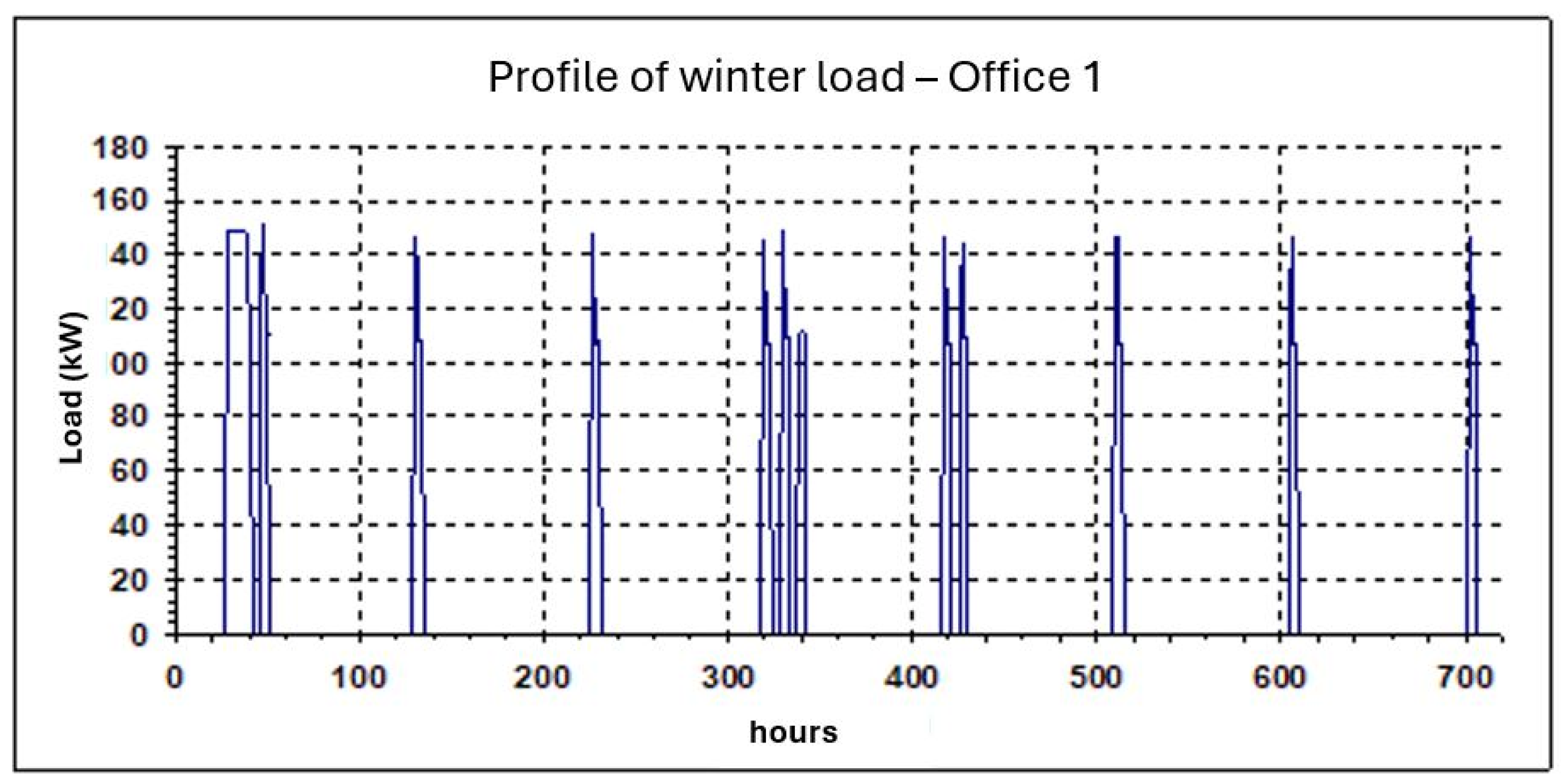
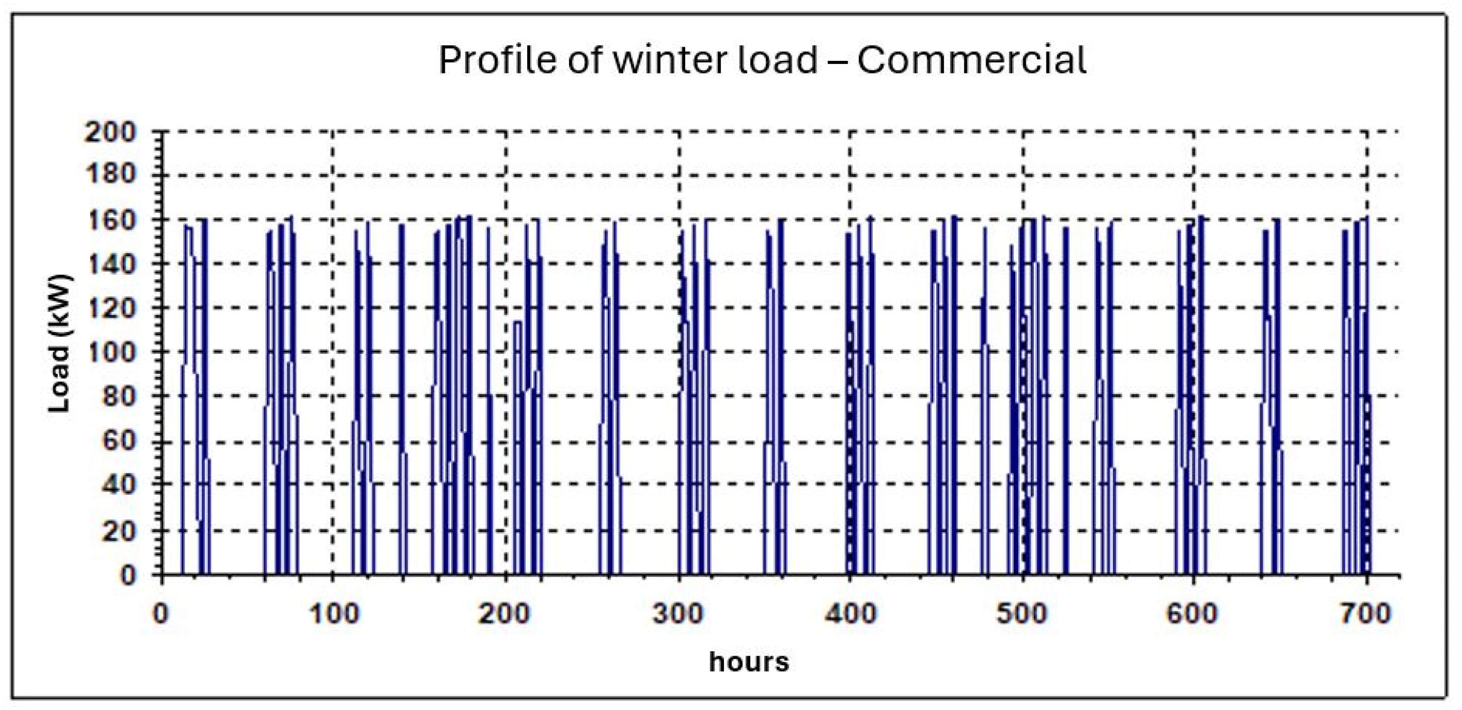
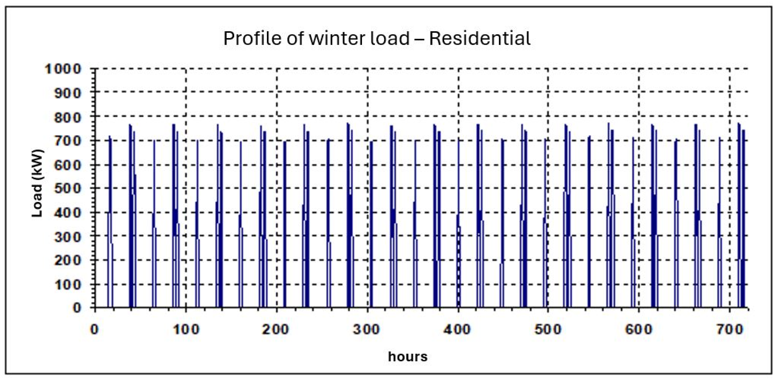
2.2. Characteristic of User Profiles and Building’s Geometry

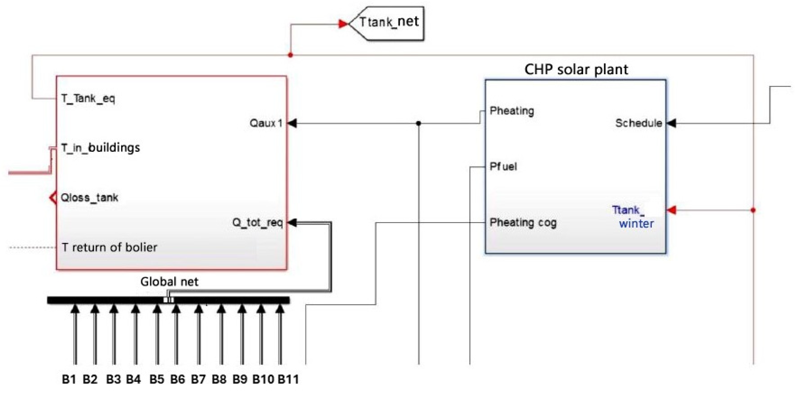
The neighborhood simulated is characterized by a mixed use of buildings: residential, commercial, and office ones. Therefore, the network is connected to eight residential buildings, two offices, and one commercial structure (

Table 2. Characteristics of the buildings connected to the district heating network.

Type of Building	Volume (m3)	Number of Floors	Total Height (m)	Number of Occupants
Res 1	14,580	12	78	4
Res 2	21,960	12	175	4
Res 3	19,110	12	192	4
Res 4	22,632	12	198	4
Res 5	22,800	15	192	5
Res 6	26,160	15	200	5
Res 7	30,912	21	140	7
Res 8	22,356	12	200	4
Office 1	3240	9	100	3
Office 2	360	3	20	1
Commercial	7650	9	250	3

).

The stratigraphy of the buildings is shown in

Table 3. Thermal transmittance proprieties of the building’s structure.

Type	Elements	Total Transmittance W/m2K
External walls	Bricks and lime	1.056
Ground slabs	Semi-rigid panels, predellas slab and floor tiles	0.438
Intermediate slabs	Semi-rigid panels, reinforced concrete layers and floor tiles	0.647
Roof covering	Semi-rigid panels, reinforced concrete layers and cement mortar	0.441

. These values were applied to all the building’s typology, a hypothesis that appears to be realistic for many Italian urban contexts.

Considering the occupational profiles, the powers relating to the lighting, the equipment and their use profiles, and the operating profile of the air conditioning system, it was possible to calculate the thermal loads of each building block, using the ODESSE software (v0.2) [29]. The temperature was set to 20 °C for the winter season and 26 °C for the summer season. As an example, Figure 2 shows the profile of the winter load of Office 1, Figure 3 shows the profile of a residential building and Figure 4 the profile of the commercial structure.

2.3. Model Setup

To define the proposed energy model, Matlab Simulink R2021b was used, to model the dynamic functioning of the district heating network. Summarizing, the configuration is composed of a single branched district heating network (one delivery and one return), with hot heat transfer fluid, specifically water, the users are therefore supplied with hot fluid both in summer and in winter. The buildings of the users will be equipped with heat exchanger substations and in the summer season, they will also be equipped with LiBr absorbers (Bro-lithium wall) to produce chilled water (becoming a distributed cooling generation system). Finally, the network is powered as already mentioned by four configurations of energy generation plants (Section 2.3.2).

2.3.1. Modelling the Building

As already mentioned, eleven buildings are connected to the network. The modelling of buildings required the definition of the following elements:

• user substation, with the exchanger and the absorber;
• hot storage and cold storage;
• electric charge;
• DHW block;
• the two load profiles, summer, and winter;
• “T out, winter” and “T out, summer” which describe the behavior of the distribution system by delivering the outlet temperature from the terminals.

The building inlet temperature, i.e., the temperature at which the network supplies water to the buildings, is the main actor. The heat exchanger generates the output power that the network will deliver to the building. The pursuit between the two powers is carried out by the winter tank and the summer tank. By monitoring the temperature of the buildings’ tanks (the thermal storage) and checking that they are close to the required values, the “tracking” between the two powers (required by the building and given by the network) is guaranteed.

User’s substation: The powers of the user exchangers of the 11 building blocks were calculated by analyzing the load profile of the buildings themselves; the power of the exchanger was set equal to the maximum power required by the building considered. The temperature between the delivery and return of the network is set at 10 °C. The necessary flow rate is obtained in winter, which is constant but different from building to building. It is guaranteed that no more power is extracted from the exchanger than is necessary for the needs and thermal load of the building. The outlet temperature of the water from the user is obtained as follows Equation (3):

$$T_{out,users }=T_{in}+{\displaystyle \frac{P_{exchanger}}{P_{CFR}{C}_p}} [°\mathrm{C}]$$

(3)

where P_FCR is the flow rate of the water circulating in the fan coil, P_exchanger is the power of the substation, c_p is the specific heat of water, and T_out,users and T_in are the inlet and outlet temperatures, respectively.

Moving to the summer season, the absorber is connected directly to the network, and the temperature of the water leaving the machine is calculated as Equation (4) and the exchanged power as Equation (5):

$$T_{out network }=T_{in network }-5 [°\mathrm{C}]$$

(4)

$$P_{th }=G_{absorber }-C_p∆T \left[\mathrm{kW}\right]$$

(5)

where T_{in network} is the temperature of the network, and G_absorbed is the flow rate in the absorber.

Thermal storage: It was verified, during the simulation phase, that a correct volume of storage is essential to obtain the proper temperature of the volume. In the simulations, the storage volumes of all the users were considered. The dynamics of thermal storage is governed by the following differential Equation (6):

$${\displaystyle \frac{dT}{dt}}={\displaystyle \frac{Q_{aux}-Q_{load}-(K_{storage} {FF}_{storage}{V}_{storage}\left(T_t-T_{amb}\right))}{C_p\rho V_{storage}}}$$

(6)

where:

−

Q_load is the load of the users connected to the network;

−

Q_aux is the thermal load supplied to the tank by the heat exchanger;

−

K_storage is the thermal transmittance of the thermal storage;

−

FF_storage is the storage form factor;

−

T_t is the temperature of the storage;

−

T_amb is the ambient temperature;

−

ρ is the density of the water;

−

V_storage is the volume of the storage.

2.3.2. Modelling the Networks and the Energy Generation Systems

Figure 5 shows the network which has an input power that the systems transfer to the network itself and the power that the 11 building blocks request from the network. At the output, the network provides the temperatures at the entrance to the buildings, in the various branches, and the temperature of the network tank.

The thermal model of the network provides the output temperature value that occurs in each node of the network, delivery and return, the time–domain trend of the temperature, and the energy losses along the network. Once the temperature of the fluid entering the network is known, it is possible to calculate the temperature trend along the entire district heating network and the derivation nodes entering the substations of each building, according to Equation (7):

$$T_{(x,t)}=T_t+\left(T_{0,t}-T_t\right)e^{{\displaystyle \frac{-2\pi H}{G\gamma }}x} [°\mathrm{C}]$$

(7)

where:

−

T_t, is the temperature of the soil [°C];

−

T_0,t, is the node’s temperature [°C];

−

G, pipe’s flow rate [kg/s];

−

r, medium radius of the pipe [m];

−

γ, specific heat [J/kgK];

−

H, pipe’s transmittance [W/m²K];

−

x, pipe’s length [m].

Equation (7) is based on the following hypotheses: stationary regime, uniform temperature along the section, i.e., the temperature varies only along the x-axis (one-dimensionality of the flow) and constant thermophysical properties as the temperature varies. To calculate the losses in the return branches of the network, the mixing temperature was calculated in each node of the return network as follows Equation (8):

$$T_{node}={\displaystyle \frac{{\sum }_n{T}_n{m}_n}{\sum _n{m}_n}}v [°\mathrm{C}]$$

(8)

where T_n and m_n are the temperature and mass rate of the segment, respectively, and v is the velocity. The flow rate losses were calculated as Equation (9):

$$Q_{loss}=G_x{C}_{p }{∆T}_x \left[\mathrm{J}\right]$$

(9)

where G_x is the flow rate, C_p is the specific heat of the water and ΔT_x is the temperature difference of the segment. Equation (10) describes the network thermal storage functioning.

$${\displaystyle \frac{dT}{dt}}={\displaystyle \frac{Q_{aux}-Q_{load}-\left(\right({{sup}_{storage}K}_{storage} \left(T_t-T_{amb}\right))/1000)}{C_p\rho (V_{storage RE }+V_{storage CE})}}$$

(10)

where:

−

Q_load is the load of the users connected to the network;

−

Q_aux is the thermal load supplied to the tank by the heat exchanger;

−

K_storage is the thermal transmittance of the thermal storage;

−

FF_storage is the storage form factor;

−

T_t is the temperature of the storage;

−

T_amb is the ambient temperature;

−

ρ is the density of the water;

−

V_{storage RE} represents the volume of water present in the entire district heating network for both the flow and return;

−

V_{storage CE} is the storage volume.

Boiler system: Two boiler options were simulated (traditional and condensing), distinguishing two power categories, greater than 50 kW or less than 50 kW. The efficiency of the traditional boiler is set equal to 0.92 if the boiler power is greater than 50 kW, while for lower powers the efficiency can vary from 0.87 to 0.92. A thermostat was defined in the simulation which forces the boiler to deliver power when the network tank temperature is below the value of 90 °C and to deactivate when the network tank temperature value is greater than 95 °C. The thermostat returns a value of 1 if the boiler must provide power and 0 otherwise. If the system sees a network tank temperature of 89.9 °C it will deliver power for 15 consecutive minutes, on the contrary, if it sees a temperature of 94.9 °C it will not deliver power for 15 min.

Cogeneration plant: The cogeneration system is based on a gas-powered internal combustion engine. At the entrance of the water–water exchanger, which operates in countercurrent, there is water coming from the engine and from the network tank. Within the internal combustion engine (ICE) block, there are two other blocks. One block represents the water–water heat exchanger, capable of recovering the thermal energy from the engine cooling circuit, and a water-fume one, capable of recovering heat from its exhaust system. The water coming from the network tank will pass through the water–fume exchanger, raising its temperature even further. The engine cooling fluid will instead return to the engine core again repeating its cycle. The minimum ΔT between the water coming from the mains and the fluid returning to the engine is set equal to 5 °C. The final power of the cogeneration plant is calculated as Equation (11):

$$P_{th\_CHP }=G_{water,ICE,users }{C}_{pH2O}\left({\displaystyle \frac{T_{out,exchanger}}{f}}-T_{tank,network}\right) [\mathrm{kW}]$$

(11)

where:

−

G_{water,ICE users}, is the water flow rate of the users;

−

C_pH2O is the heat capacity of the water;

−

T_{out,exchanger} is the temperature of the water leaving the water–fume exchanger, i.e., the temperature at which the cogenerator can bring the water which then returns to the network tank;

−

T_tank,network is the temperature of the network tank, i.e., the inlet temperature to the system cogeneration and therefore to the water–water exchanger.

Solar system: the solar system communicates with the network through the power that is delivered to it, but also with the temperature of the network tank which returns to the solar system. First, it is necessary to describe two implemented control systems. In fact, during the simulation phase, where the solar block was used, it was observed that the temperatures of the network tank were not kept adequately under control, especially when the solar radiation was higher. Inside the solar block, there is already a control, e.g., a heat sink, which does not allow the solar to reach temperatures above 120 °C. This control allows the solar field to operate in optimal conditions but does not efficiently connect the grid with the solar system. To carry out this function, an additional control was implemented, that can communicate with the solar system and the grid. In this way, the solar system feeds the power into the grid that is adequate for the conditions required.

The simulations were carried out first by setting 1400 collectors (collectors with an incident surface of 10 m² and able to deliver 7000 kW), such to satisfy the needs of the network. Once the optimal V_{storage CE} was found, the number of panels was varied so that the power varied by ±20%, keeping the optimal V_{storage CE} fixed. The range of the V_{storage CE} is from 60 m³ up to 150 m³. In the simulations carried out (16 in total), the solar system works with set points equal to 80 °C in winter and 90 °C in summer, equal to the temperature of the network.

Combined solar and cogeneration plant: The best configuration must be found from the point of view of the stability of the network and its correct functioning, to maximize the use of the solar source. The parameters involved are the power of the cogeneration plant, the number of solar collectors, and the sizing of the network tank. To find the proper coupling and sizing of the sources, 15 simulations were carried out (all with solar control set to a range of 10 °C and with a T _0,summer = 90 °C and T _0,winter = 80 °C).

2.4. Exergy Indicator

Once the exergy values associated with each product and resource for each physical component of the plant were defined [6,8], the exergy efficiency indicator can be calculated as follows (Equation (12)).

$$\mathrm{Exergy} \mathrm{efficiency}: \eta ={\displaystyle \frac{{\Psi }_p}{{\Psi }_r}}={\displaystyle \frac{Exergy of the product}{Exergy of the resource}}$$

(12)

3. Results

3.1. Boiler Configuration

The simulations with the boiler system were carried out by setting the power for the boiler, equal to 7000 kW. The first step was to study the optimal accumulation volume (V_{storage CE}). Once the value of V_{storage CE} was determined, the boiler’s power was varied ±20%. Then, four volumes of storage were analyzed, equal to 45 m³, 60 m³, 90 m³, and 150 m³. As mentioned in the methodology section, the boiler works with set point temperatures between 90 °C and 95 °C. Figure 6 shows the temperature trend per each volume of the storage.

Based on the boiler volume’s temperature trend, the configuration in Figure 6c (volume of 90 m³) is the best scenario. The case with 90 m³ presents a more contained oscillation in the amplitude between minimum and maximum temperature compared to the other cases with different accumulation volumes (a) and (b). Compared to case (d), the latter is worse because it presents too frequent oscillations compared to case (c) and therefore a greater temperature variability over time.

The exergy efficiency is the sum of the main components’ exergy efficiency such as the building’s heat exchangers, the adsorber and the building, the network, and the boiler (

Table 4. Results of exergy indices calculated for the configuration.

Building Connected to the Network	Exergy Efficiency (%)
1	0.35
2	0.39
3	0.37
4	0.41
5	0.41
6	0.38
7	0.40
8	0.40
9	0.41
10	0.40
11	0.38

).

The optimal storage volume is 90 m³ as the exergy efficiency of the eleven buildings demonstrated. Then, the power was varied by ±20%, keeping the optimal storage volume. The network tank’s temperature trends were analyzed (Figure 7). Based on Figure 7, the temperature trend of the case b (boiler of 700 kW) shows few fluctuations compared to the other configurations. A high number of fluctuations mean that the boiler switches on/off frequently, thus increasing consumption, but at the same time decreasing the useful life of the apparatus.

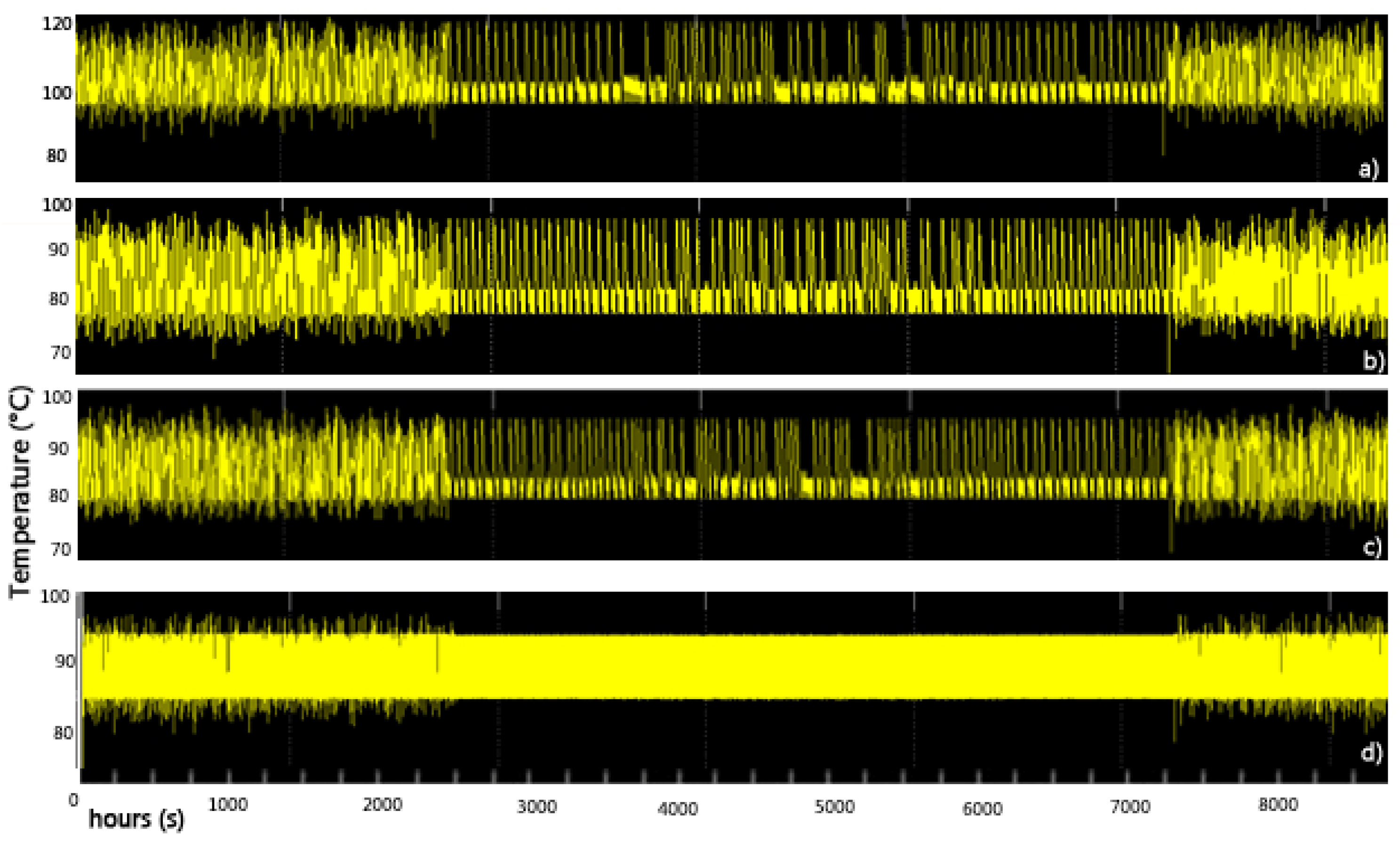
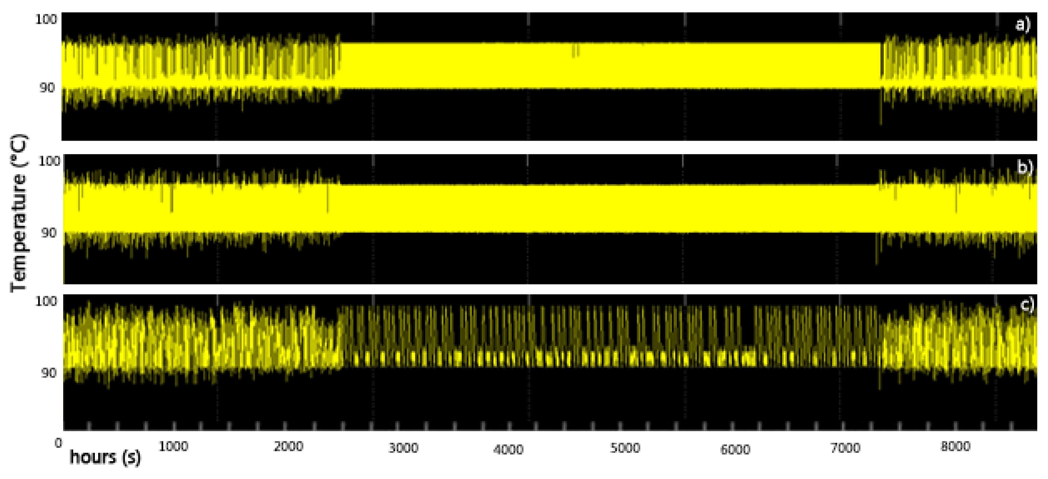
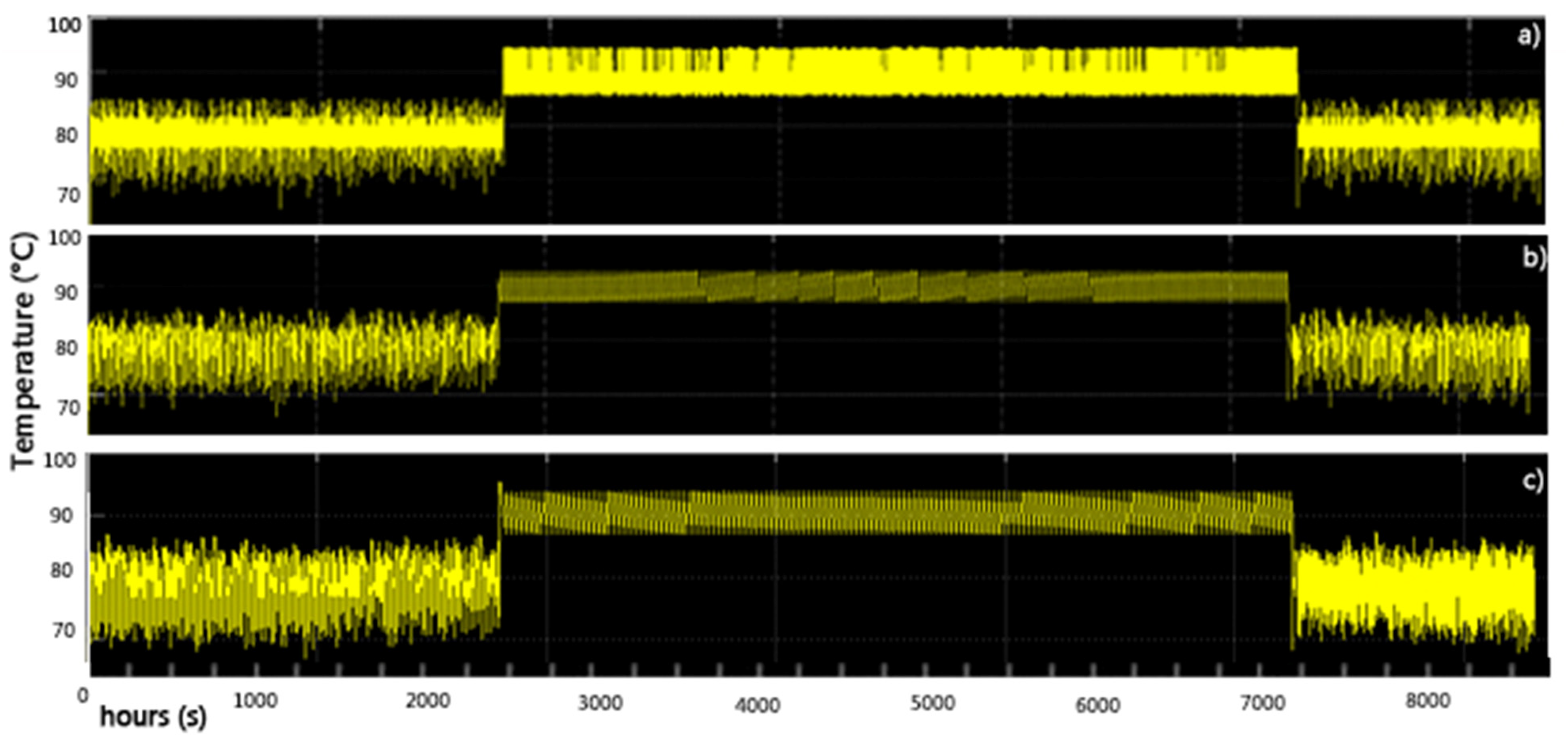
3.2. Centralizer Solar System Configuration

Several simulations were performed to define the optimal number of solar collectors equal to 1400 that are able to supply a power of 700 kW (the district heating energy requirements). Then, three volumes of the storage were investigated (Figure 8, Figure 9 and Figure 10). The solar system’s temperature setpoints are 90 °C and 80 °C in summer and winter, respectively.

Employing the solar source, the temperature trend of all the configurations is appropriate during the summer season, but not in the winter one. The solar panel system is coupled to a traditional source to improve the stability of the network, and this is confirmed by the simulations carried out (see Section 3.4). However, the best volume of the tank is described in Figure 9 (volume of 90 m³), because the amplitude of the temperature oscillations is smaller than in the case with 60 m³ but at the same time the oscillation frequency is lower than in the case with a 120 m³ tank. As it was conducted with the other energy systems, the power was varied ±20% as well as the number of collectors (1100, 1400, and 1700 panels). Figure 11, Figure 12 and Figure 13 show the results in terms of temperature during the year.

The case with 1400 solar collectors is the best possible for the network, even if not sufficient for the proper functioning throughout the year. By first analyzing the temperature of the network tank, the sizing with 1100 panels does not allow the functioning of the network, not even during the summer season (e.g., temperature below 60 °C on specific days). Then, increasing the number of panels up to 1700 does not allow more benefits compared to 1400 panels. Keeping fixed the configuration with 1400 panels,

Table 5. Results of the exergy indices for the three solar system configurations.

Building	Exergy Efficiency (%) Configuration with 1100 Panels	Exergy Efficiency (%) Configuration with 1400 Panels	Exergy Efficiency (%) Configuration with 1700 Panels
Building 1 (res)	0.24	0.17	0.09
Building 2 (office)	0.08	0.1	0.23
Building 3 (commercial)	0.18	0.13	0.19

reports the total exergy efficiency of three representative buildings connected to the network. The exergy efficiency reported is the sum of the exergy efficiency of all the elements (adsorber, heat exchanger, building, network, and solar system).

The optimum number of collectors would be 1700 panels for commercial and offices, while for residential buildings 1100 panels would be the case with the highest efficiency (Table 5). The right compromise, also given the higher number of residential buildings present in the network, appears to be the choice of 1400 panels.

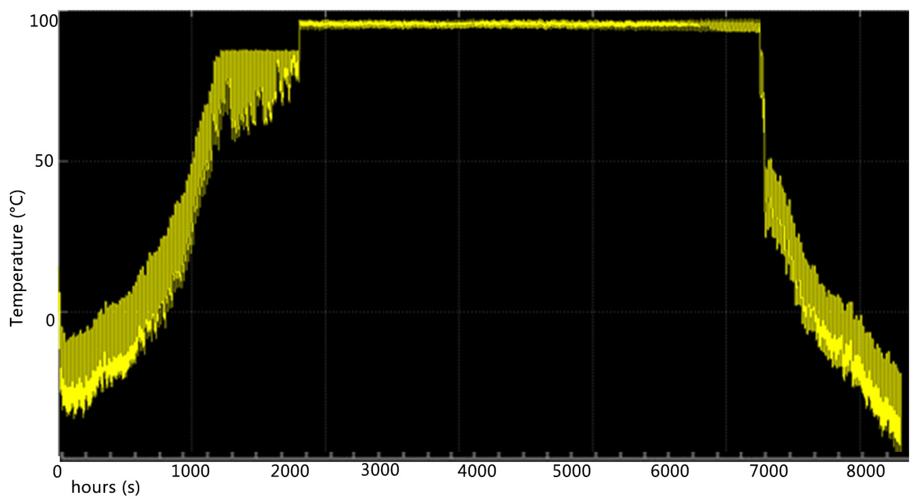
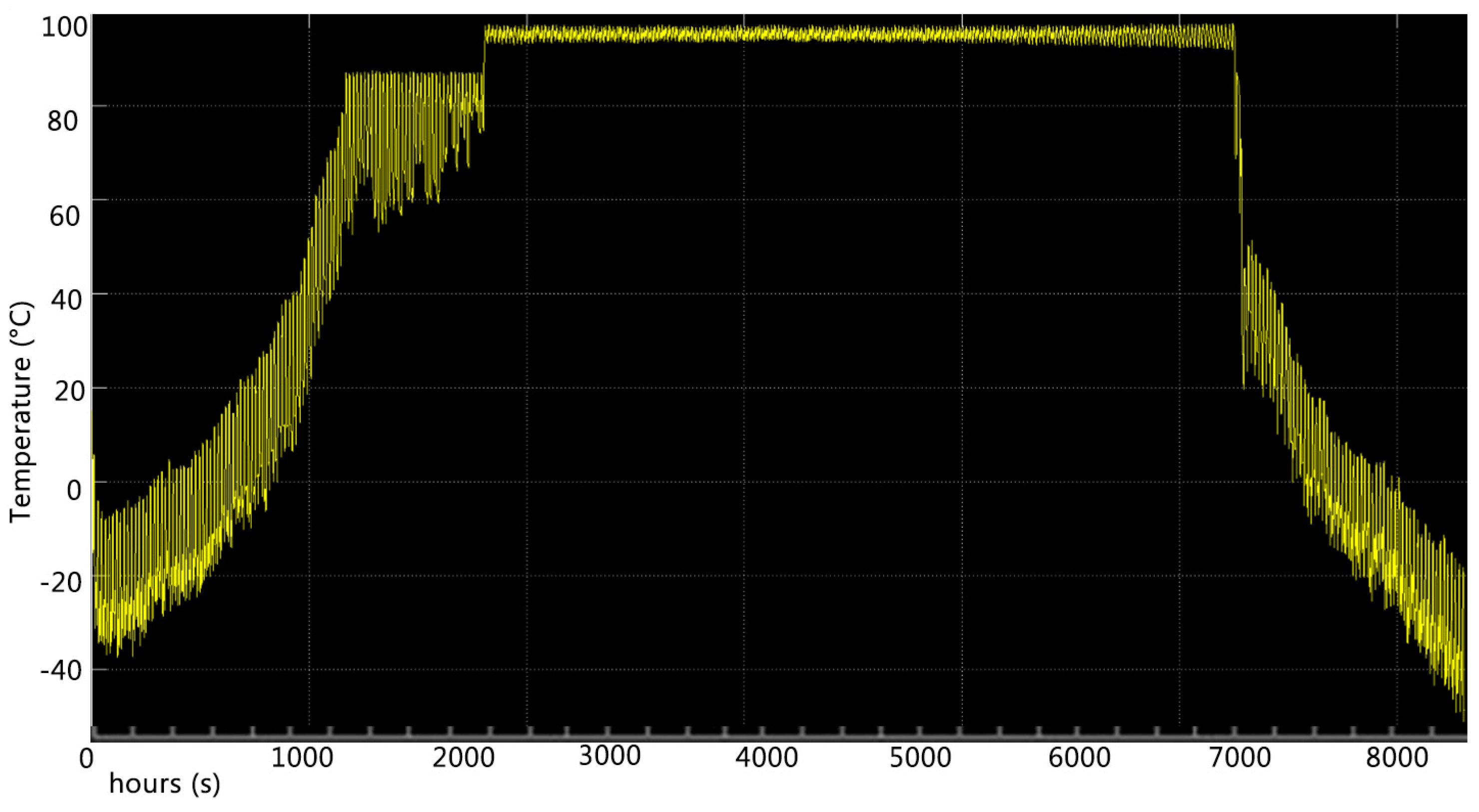
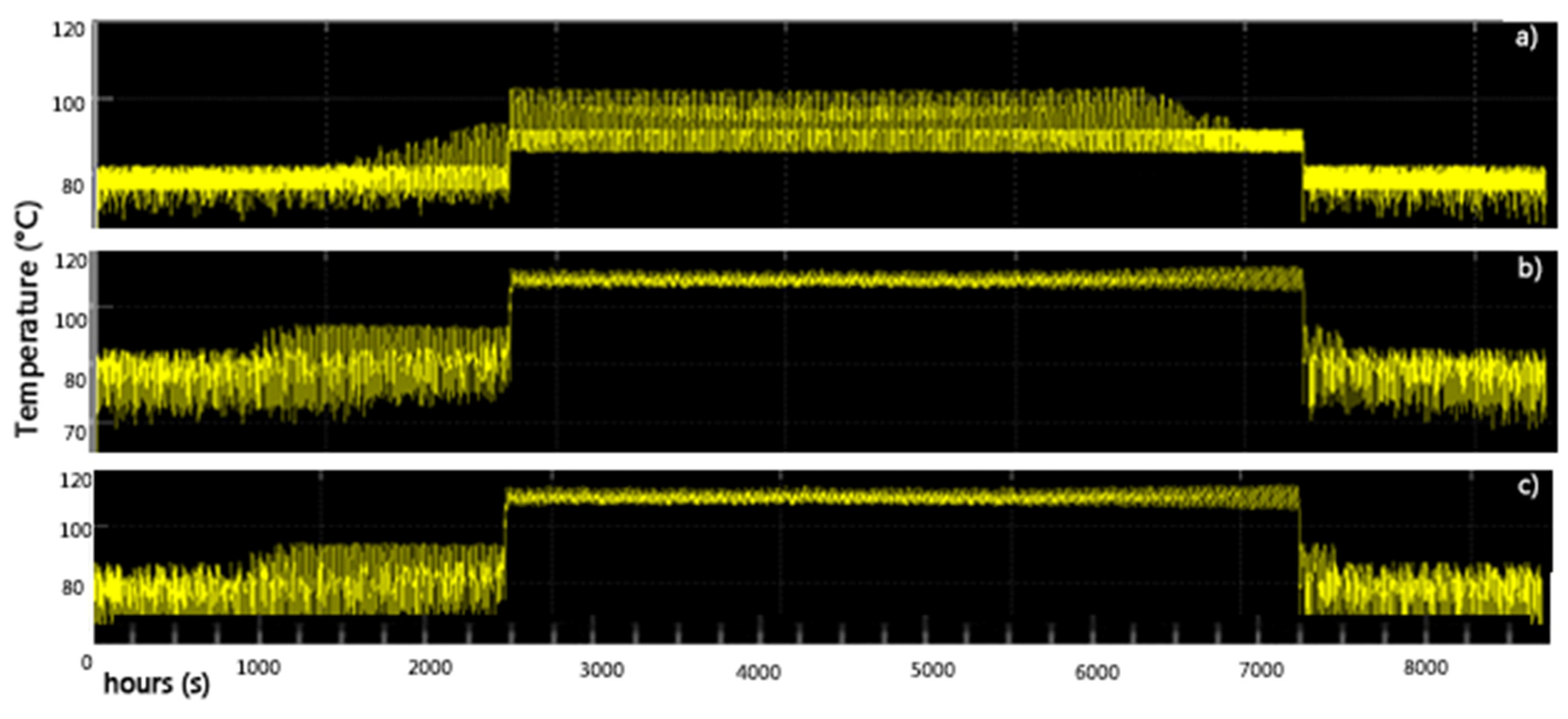
3.3. CHP Configuration

Moving to the simulations of the CHP system, the optimal network storage volume (V_{storage CE}) found for the case with the boiler was considered, equal to 90 m³, then varying the CHP power, 5600 kW, 7000 kW, and 8400 kW. The network supply temperature required by the CHP unit is 80 °C in winter and 90 °C in summer. Figure 14 reports the temperature trend of the analyzed system, keeping the storage volume (90 m³).

As shown in Figure 14, the power of 7000 kW is the minimum power that guarantees good functioning of the system, also visible from the temperature trend of the network storage. Moving to the exergy evaluation,

Table 6. Results of the exergy indices for the three CHP power configurations.

Building	Exergy Efficiency (%) The Power of CHP Is 5600 kW	Exergy Efficiency (%) The Power of CHP Is 7000 kW	Exergy Efficiency (%) The Power of CHP Is 8400 kW
Building 1 (res)	0.35	0.35	0.36
Building 2 (office)	0.42	0.41	0.42
Building 3 (commercial)	0.38	0.38	0.38

collects the exergy efficiency of the tree configurations analyzed for the three selected buildings. Looking at Table 6, there are no obvious differences between the three CHP sizes for each type of building.

3.4. Solar System and CHP Configuration

The simulations were carried out by setting a power for the CHP equal to 3500 kW and employing 700 collectors. The first step is to set the optimal volume of storage between four values: 60 m³, 90 m³, 120 m³, and 150 m³. The temperature supplied to the systems is 80 °C in winter and 90 °C in summer. Figure 14 shows the temperature results of each case.

Based on Figure 15, the optimal storage volume is 120 m³, which shows the best temperature trend of the network tank. The combination of CHP and solar systems allow the instability of renewable energy sources (case with the solar system alone) to be overcome. This fact is also visible by analyzing the temperatures of the network’s storage, which are very stable and able to satisfy user requests. Summarizing the optimal volumes of the latest three energy systems are as follows:

−

120 m³ for the CHP and solar system configuration (Figure 15).

−

90 m³ for the CHP alone.

−

150 m³ for the solar system alone.

Once the optimal volume was set (120 m³), the power of the system was varied as well as the number of panels (Figure 15). Three configurations were taken into consideration as reported below (Figure 16).

• The power of CHP is equal to 2800 kW with 520 panels.
• The power of CHP is equal to 3500 kW with 700 panels.
• The power of CHP is equal to 4200 kW with 840 panels.

There are no obvious differences between the configuration with 700 panels and 840 panels; therefore, for the same performance, the configuration with the certainly lower cost is chosen. Finally,

Table 7. Results of the exergy indices for the three energy systems configurations.

Building	Exergy Efficiency (%) CHP of 3500 kW and 700 Panels	Exergy Efficiency (%) CHP of 2800 kW and 520 Panels	Exergy Efficiency (%) CHP of 4200 kW and 840 Panels
Building 1 (res)	0.35	0.36	0.36
Building 2 (office)	0.41	0.41	0.41
Building 3 (commercial)	0.39	0.40	0.40

reports the main exergy results of the selected buildings.

Also in this case, when analyzing the three types of buildings present in the network, no significant differences are noted by changing the size of the CHP and the number of panels. The exergy analysis performed on the individual buildings does not lead to understanding what the optimum of the configurations is considered. Therefore, it is obvious that together with the exergy analysis, a more in-depth analysis carried out on the temperatures of the network and the various components must be coupled.

4. Conclusions

A growing global population and the depletion of fossil fuels are driving the need for sustainable energy systems. Buildings are being designed to reduce their environmental footprints using alternative and sustainable approaches due to the current energy transition. In this framework, the proposed study evaluates the optimal energy and storage systems to feed a district heating network. A model based on Matlab/Simulink was established. Four types of energy systems were analyzed, such as traditional boilers, CHP technology, solar systems, and cogeneration plant with solar system. Thermal energy storage of the network is investigated in terms of volume and temperature.

The optimal storage volume of the scenario with boilers is 90 m³. Then, the selected power of boiler is 700 kW, because it shows few fluctuations compared to the other configurations (5600 kW and 7400 kW). Moving to the solar system, the best configuration is obtained with a thermal storage of 90 m³ and 1400 solar collectors. To define the optimal number of solar collectors (1100, 1400 and 1700 units), exergy analysis was employed. Based on the exergy efficiency of commercial and office buildings (0.19% and 0.23%), the optimum number is 1700 panels, while for residential buildings it is 1100 panels with an exergy efficiency of 0.24%. The proper compromise seems to be the choice of 1400 panels, due to the mixed-use of buildings connected to the network. The cogeneration plant system of 7000 kW is the minimum power that guarantees the proper functioning of the system compared to the other two sizes (5600 kW and 7400 kW). Regarding the exergy efficiency, there are no relevant differences between the three cogeneration plant sizes for each type of building. Finally, the combination of cogeneration plants and solar systems shows a good temperature trend when a storage volume of 120 m³ is employed. Then, three sizes of cogeneration plants were performed (2800, 3500 and 4200 kW) combined with different numbers of panels (540, 700, 840 panels). No relevant variations between the configuration with 700 panels and 840 panels were detected; therefore, for the same performance, the configuration with the lower cost is chosen. In line with this, the best heating system configuration to feed the studied district heating is the cogeneration plant with and solar collectors, according to the energy and exergy point of view. The storage system applied to this configuration is suitable for managing the fluctuation of renewable energy resources.

However, the exergy efficiency alone, especially for the third configuration, is not able to identify the difference in the “quality of the energy” of each component of the grid (buildings and so on); therefore, the analysis of the temperature of the network and the storage is crucial during the first stage of analysis. It is recommended to further investigate another type of exergy indicator that can contribute to improving the performances of such energy systems for the built environment.

References

1. Giuzio, G.F.; Forzano, C.; Barone, G.; Buonomano, A. Accelerating the Low-Carbon Transition: Technological Advancements and Challenges for the Sustainable Development of Energy, Water, and Environment Systems. Energy Rep. 2024, 11, 4676–4687. [Google Scholar] [CrossRef]
2. Barone, G.; Buonomano, A.; Forzano, C.; Giuzio, G.F.; Palombo, A. Assessing Energy Demands of Building Stock in Railway Infrastructures: A Novel Approach Based on Bottom-up Modelling and Dynamic Simulation. Energy Rep. 2022, 8, 7508–7522. [Google Scholar] [CrossRef]
3. Halkos, G.E.; Gkampoura, E.C. Reviewing Usage, Potentials, and Limitations of Renewable Energy Sources. Energies 2020, 13, 2906. [Google Scholar] [CrossRef]
4. Lu, Y.; Khan, Z.A.; Alvarez-Alvarado, M.S.; Zhang, Y.; Huang, Z.; Imran, M. A Critical Review of Sustainable Energy Policies for the Promotion of Renewable Energy Sources. Sustainability 2020, 12, 5078. [Google Scholar] [CrossRef]
5. Terés-Zubiaga, J.; Jansen, S.C.; Luscuere, P.; Sala, J.M. Dynamic Exergy Analysis of Energy Systems for a Social Dwelling and Exergy Based System Improvement. Energy Build 2013, 64, 359–371. [Google Scholar] [CrossRef]
6. Dincer, I. The Role of Exergy in Energy Policy Making. Energy Policy 2002, 30, 137–149. [Google Scholar] [CrossRef]
7. García Kerdan, I.; Raslan, R.; Ruyssevelt, P.; Morillón Gálvez, D. The Role of an Exergy-Based Building Stock Model for Exploration of Future Decarbonisation Scenarios and Policy Making. Energy Policy 2017, 105, 467–483. [Google Scholar] [CrossRef]
8. Nardecchia, F.; Pompei, L.; Egidi, E.; Faneschi, R.; Piras, G. Exergoeconomic and Environmental Evaluation of a Ground Source Heat Pump System for Reducing the Fossil Fuel Dependence: A Case Study in Rome. Energies 2023, 16, 6167. [Google Scholar] [CrossRef]
9. Evola, G.; Costanzo, V.; Marletta, L. Exergy Analysis of Energy Systems in Buildings. Buildings 2018, 8, 180. [Google Scholar] [CrossRef]
10. Tsatsaronis, G. The Future of Exergy-Based Methods. Energy 2024, 302, 131881. [Google Scholar] [CrossRef]
11. Nardecchia, F.; Groppi, D.; Lilliu, I.; Astiaso Garcia, D.; De Santoli, L. Increasing Energy Production of a Ducted Wind Turbine System. Wind Eng. 2020, 44, 560–576. [Google Scholar] [CrossRef]
12. Al-Shetwi, A.Q.; Hannan, M.A.; Jern, K.P.; Mansur, M.; Mahlia, T.M.I. Grid-Connected Renewable Energy Sources: Review of the Recent Integration Requirements and Control Methods. J. Clean. Prod. 2020, 253, 119831. [Google Scholar] [CrossRef]
13. Lygnerud, K.; Fransson, N.; Särnbratt, M.; Motoasca, E.; Neven, T.; Vanschoenwinkel, J.; Pastor, C.; Gabaldón, A.; Belda, A. District Energy Viewed from the New Bauhaus Initiative Perspective—Sustainable, Inclusive and Aesthetic Heat. Buildings 2023, 13, 2930. [Google Scholar] [CrossRef]
14. Li, X.; Li, Y.; Zhou, H.; Fu, Z.; Cheng, X.; Zhang, W. Research on the Carbon Emission Baselines for Different Types of Public Buildings in a Northern Cold Areas City of China. Buildings 2023, 13, 1108. [Google Scholar] [CrossRef]
15. Ponechal, R.; Jandačka, J.; Ďurica, P. Evaluation of Residential Buildings Savings for Various Envelope Retrofits and Heating Energy Sources: A Simulation Study. Buildings 2024, 14, 332. [Google Scholar] [CrossRef]
16. Hirvonen, J.; Kosonen, R. Waste Incineration Heat and Seasonal Thermal Energy Storage for Promoting Economically Optimal Net-Zero Energy Districts in Finland. Buildings 2020, 10, 205. [Google Scholar] [CrossRef]
17. Ali, E.; Ajbar, A.; Lamrani, B. Numerical Investigation of Thermal Energy Storage Systems for Collective Heating of Buildings. Buildings 2024, 14, 141. [Google Scholar] [CrossRef]
18. Wahi, P.; Konstantinou, T.; Tenpierik, M.J.; Visscher, H. Lower-Temperature-Ready Renovation: An Approach to Identify the Extent of Renovation Interventions for Lower-Temperature District Heating in Existing Dutch Homes. Buildings 2023, 13, 2524. [Google Scholar] [CrossRef]
19. Ju, Y.; Hiltunen, P.; Jokisalo, J.; Kosonen, R.; Syri, S. Benefits through Space Heating and Thermal Storage with Demand Response Control for a District-Heated Office Building. Buildings 2023, 13, 2670. [Google Scholar] [CrossRef]
20. Ju, Y.; Jokisalo, J.; Kosonen, R. Peak Shaving of a District Heated Office Building with Short-Term Thermal Energy Storage in Finland. Buildings 2023, 13, 573. [Google Scholar] [CrossRef]
21. Pompei, L.; Nardecchia, F.; Mattoni, B.; Gugliermetti, L.; Bisegna, F. Combining the exergy and energy analysis for the assessment of district heating powered by renewable sources. In Proceedings of the 2019 IEEE International Conference on Environment and Electrical Engineering and 2019 IEEE Industrial and Commercial Power Systems Europe (EEEIC/I&CPS Europe), Genova, Italy, 11–14 June 2019; pp. 1–5. [Google Scholar]
22. Buonomano, A.; Forzano, C.; Palombo, A.; Russo, G. Solar-Assisted District Heating Networks: Development and Experimental Validation of a Novel Simulation Tool for the Energy Optimization. Energy Convers. Manag. 2023, 288, 117133. [Google Scholar] [CrossRef]
23. Yazici, H. Energy and Exergy Based Evaluation of the Renovated Afyon Geothermal District Heating System. Energy Build 2016, 127, 794–804. [Google Scholar] [CrossRef]
24. Sartor, K.; Dewallef, P. Exergy Analysis Applied to Performance of Buildings in Europe. Energy Build 2017, 148, 348–354. [Google Scholar] [CrossRef]
25. Gao, Y.J.; Wang, S.G.; Jiang, S.; Wu, X.Z.; Wang, J.H.; Zhang, T.F.; Ma, Z.J. Configurations and Exergy Analysis of District Heating Substations Based Mainly on Renewable Energy. In Proceedings of the E3S Web of Conferences, Xi’an, China, 16–19 September 2022; EDP Sciences: Les Ulis, France, 2022; Volume 356. [Google Scholar]
26. Causone, F.; Sangalli, A.; Pagliano, L.; Carlucci, S. An Exergy Analysis for Milano Smart City. Energy Procedia 2017, 111, 867–876. [Google Scholar] [CrossRef]
27. Kallert, A.; Schmidt, D.; Bläse, T. Exergy-Based Analysis of Renewable Multi-Generation Units for Small Scale Low Temperature District Heating Supply. Energy Procedia 2017, 116, 13–25. [Google Scholar] [CrossRef]
28. Calise, F.; Cappiello, F.L.; Cimmino, L.; Vicidomini, M.; Petrakopoulou, F. Thermoeconomic Analysis of a Novel Topology of a 5th Generation District Energy Network for a Commercial User. Appl. Energy 2024, 371, 123718. [Google Scholar] [CrossRef]
29. ODESSE Software. Available online: https://pnpe2.enea.it/odesse (accessed on 20 February 2024).
Figure 1. Simplified district heating network scheme.
Buildings 14 02370 g001
Figure 2. Example of tertiary building’s winter load profile (office 1).
Buildings 14 02370 g002
Figure 3. Example of commercial building’s winter load profile.
Buildings 14 02370 g003
Figure 4. Example of residential building’s winter load profile.
Buildings 14 02370 g004
Figure 5. Model of the network, involving the buildings and the thank.
Buildings 14 02370 g005
Figure 6. Results of temperature trend per each volume (a) volume of 45 m3; (b) volume of 60 m3; (c) volume of 90 m3; and (d) volume of 150 m3.
Buildings 14 02370 g006
Figure 7. Results of temperature trend of the network tank with boiler power of (a) 5600 kW; (b) 7000 kW; and (c) 8400 kW.
Buildings 14 02370 g007
Figure 8. The temperature trend of the tank using volume storage of 60 m3.
Buildings 14 02370 g008
Figure 9. The temperature trend of the tank using volume storage of 90 m3.
Buildings 14 02370 g009
Figure 10. The temperature trend of the tank using volume storage of 120 m3.
Buildings 14 02370 g010
Figure 11. Temperature trend of the network’s tank combined with 1100 collectors.
Buildings 14 02370 g011
Figure 12. Temperature trend of the network’s tank combined with 1400 collectors.
Buildings 14 02370 g012
Figure 13. Temperature trend of the network’s tank combined with 1700 collectors.
Buildings 14 02370 g013
Figure 14. Temperature trend of the network tank with boiler power of (a) 5600 kW; (b) 7000 kW; and (c) 8400 kW applied to CHP configuration.
Buildings 14 02370 g014
Figure 15. Results of the temperature trend of the network tank for different seizes; (a) 60 m3; (b) 90 m3; (c) 120 m3; and (d) 150 m3.
Buildings 14 02370 g015
Figure 16. Results of temperature trend of the network tank for different seizes; (a) Scenario 1; (b) Scenario 2; and (c) Scenario 3.
Buildings 14 02370 g016