
Investigating Variations in Anthropogenic Heat Flux along Urban–Rural Gradients in 208 Cities in China during 2000–2016


Abstract
1. Introduction
- Are ArUHI effects discernible in China throughout the specified period, and what nuances characterize their spatiotemporal variations?
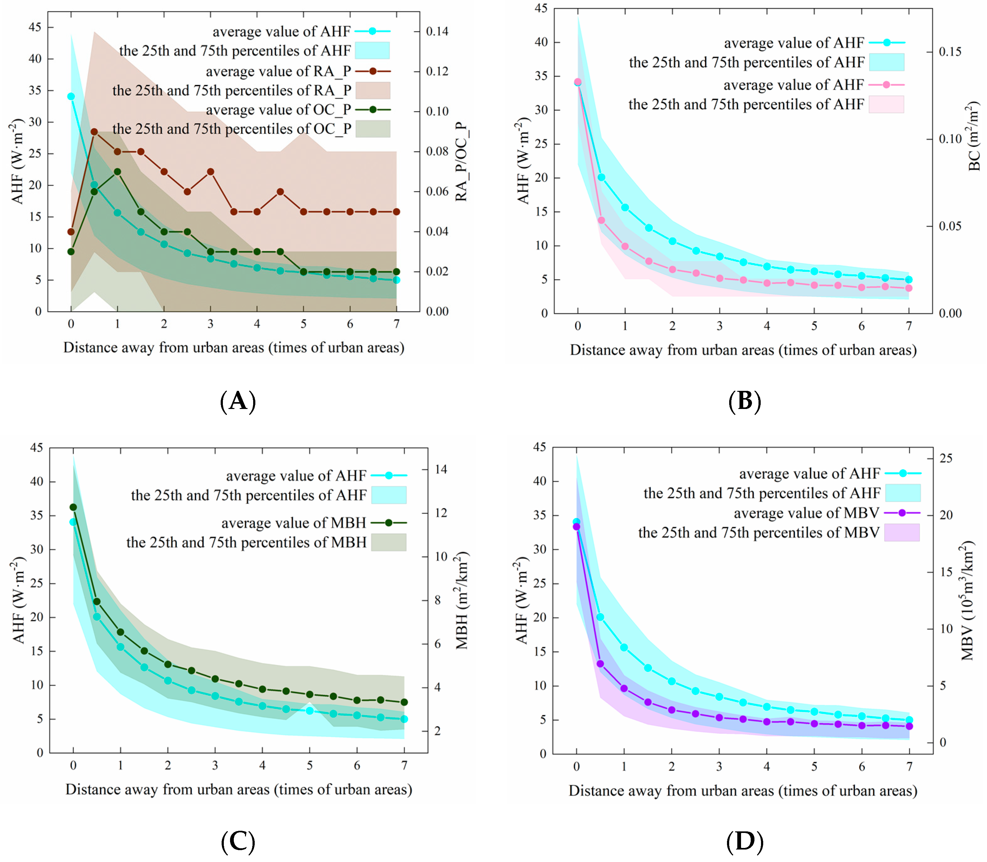
- How do the intricate interactions between land cover and building form components influence the variations in AHF along urban–rural gradients?
- To what extent can economic zones and city sizes alter the intensities and footprints of ArUHI effects?
2. Materials and Methods
2.1. Materials
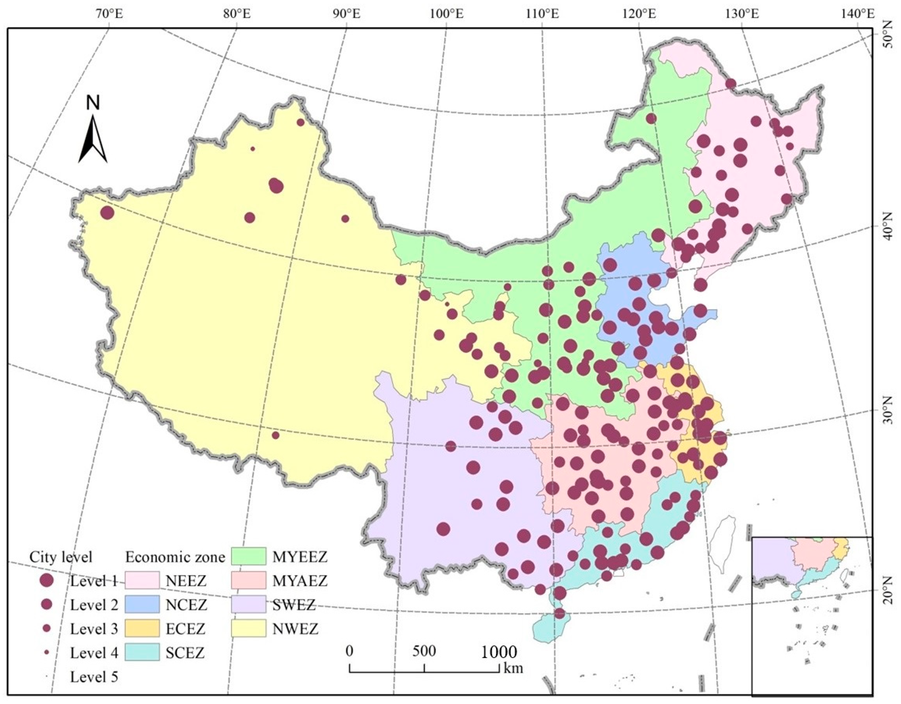
2.1.1. Study Area
2.1.2. Data Used
- AHF data
- Land use data
- Two-dimensional (2D) and three-dimensional (3D) building forms
2.2. Methods
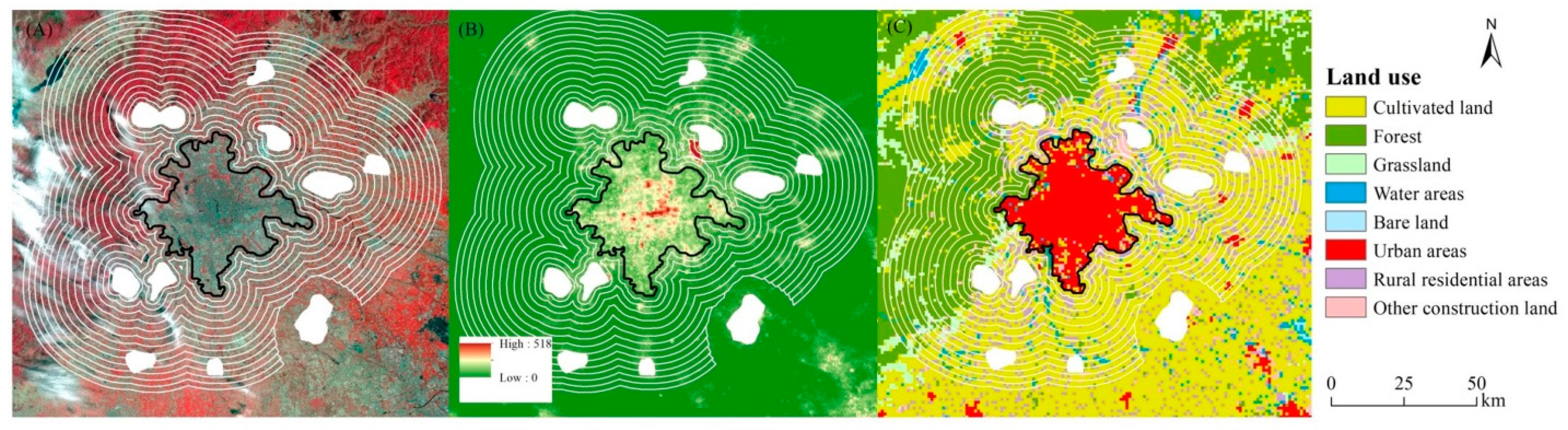
2.2.1. Delineation of Urban and Background Areas
- Utilizing the Geopandas Python library, a loop structure was implemented to iteratively generate buffer zones, which varied in size from 1.5 to 8 times the urban area. The difference in area between adjacent buffer zones was set at 0.5 times the urban area.
- The intersection of adjacent buffer zones was performed, followed by the removal of overlapping sections, resulting in 14 non-overlapping buffer zones, each with an area equivalent to half of the urban area.
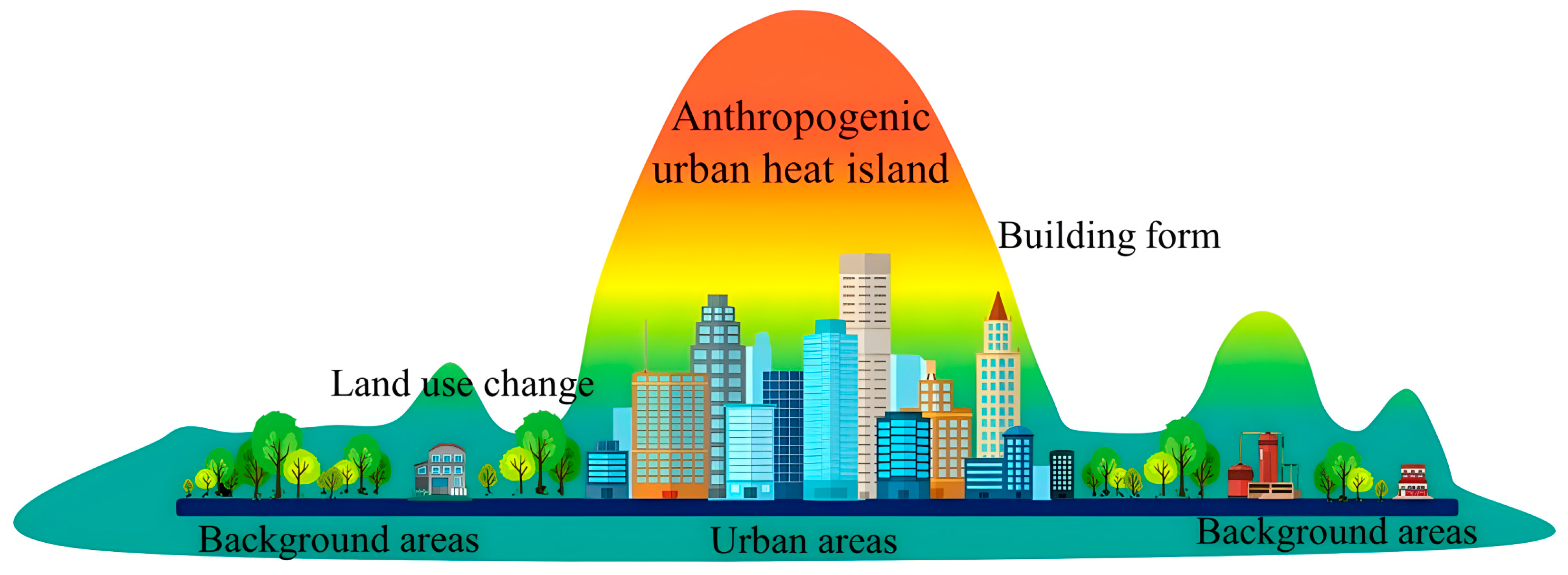
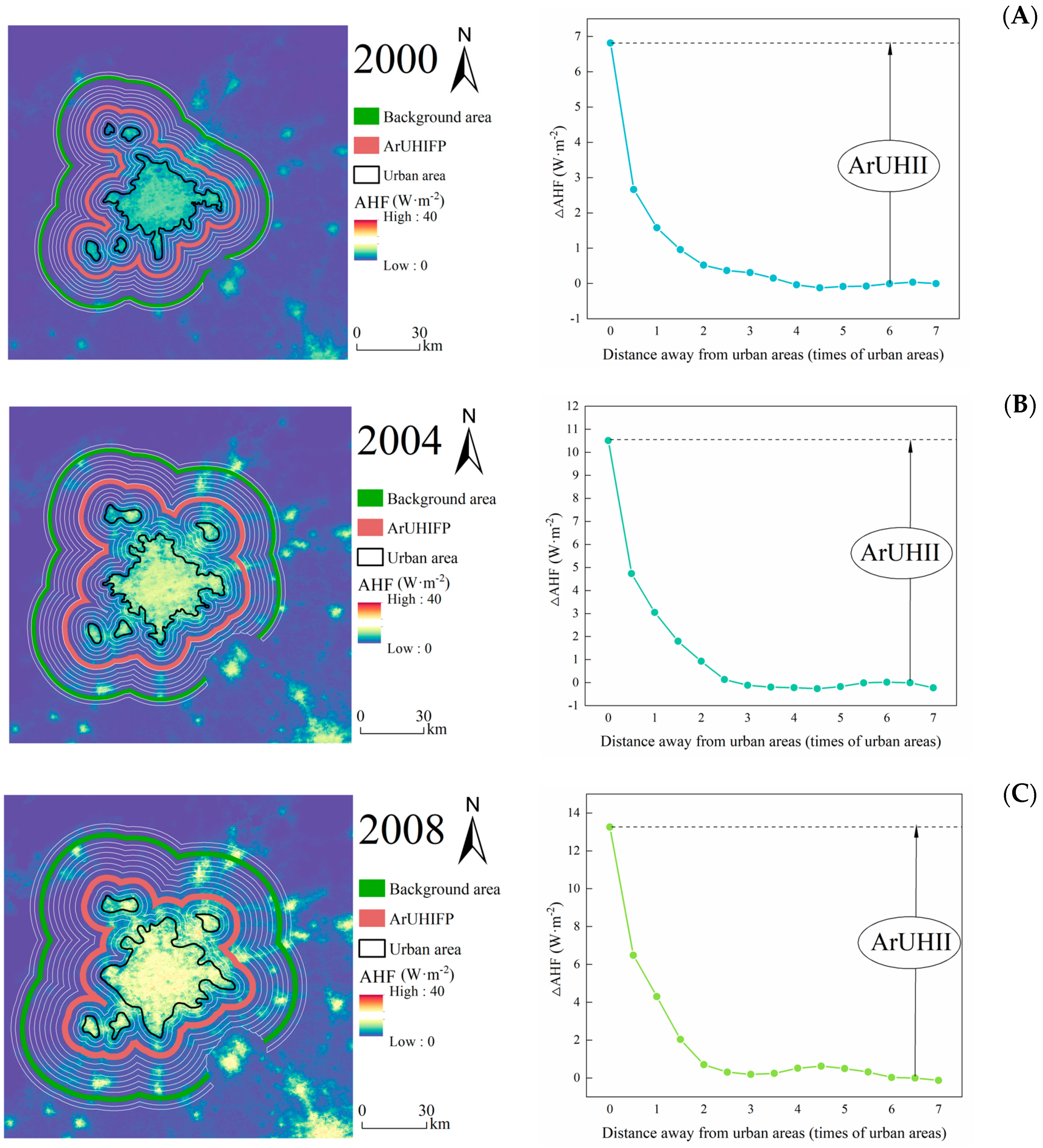
2.2.2. Definition of Anthropogenic Urban Heat Islands
2.2.3. Metrics of ArUHI: ArUHII and ArUHIFP
2.2.4. Statistical Analysis
- Selection of the influencing factors
- Statistical analyses
3. Results
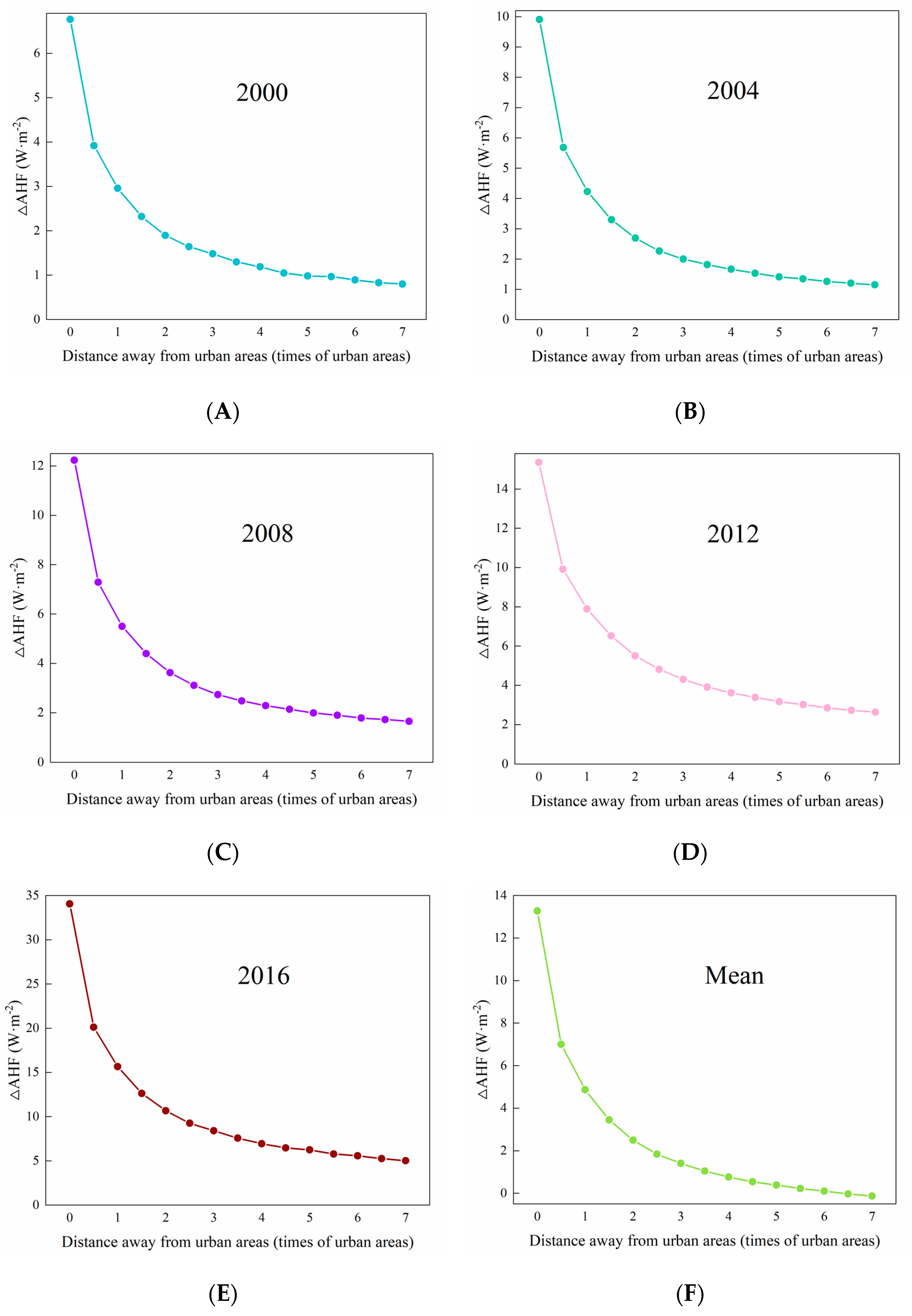
3.1. Exponential Decay of ArUHIs along Urban-Rural Gradients
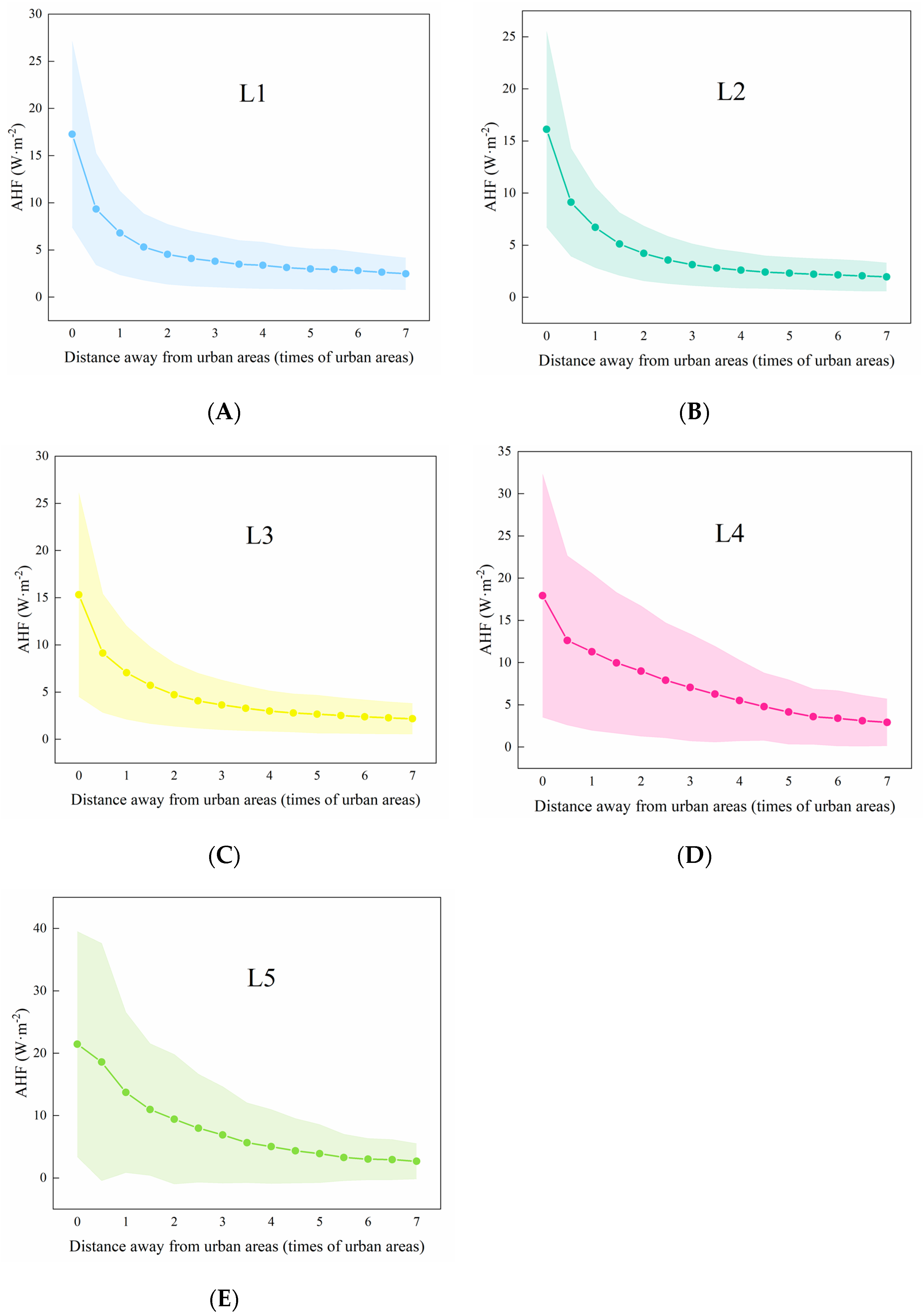
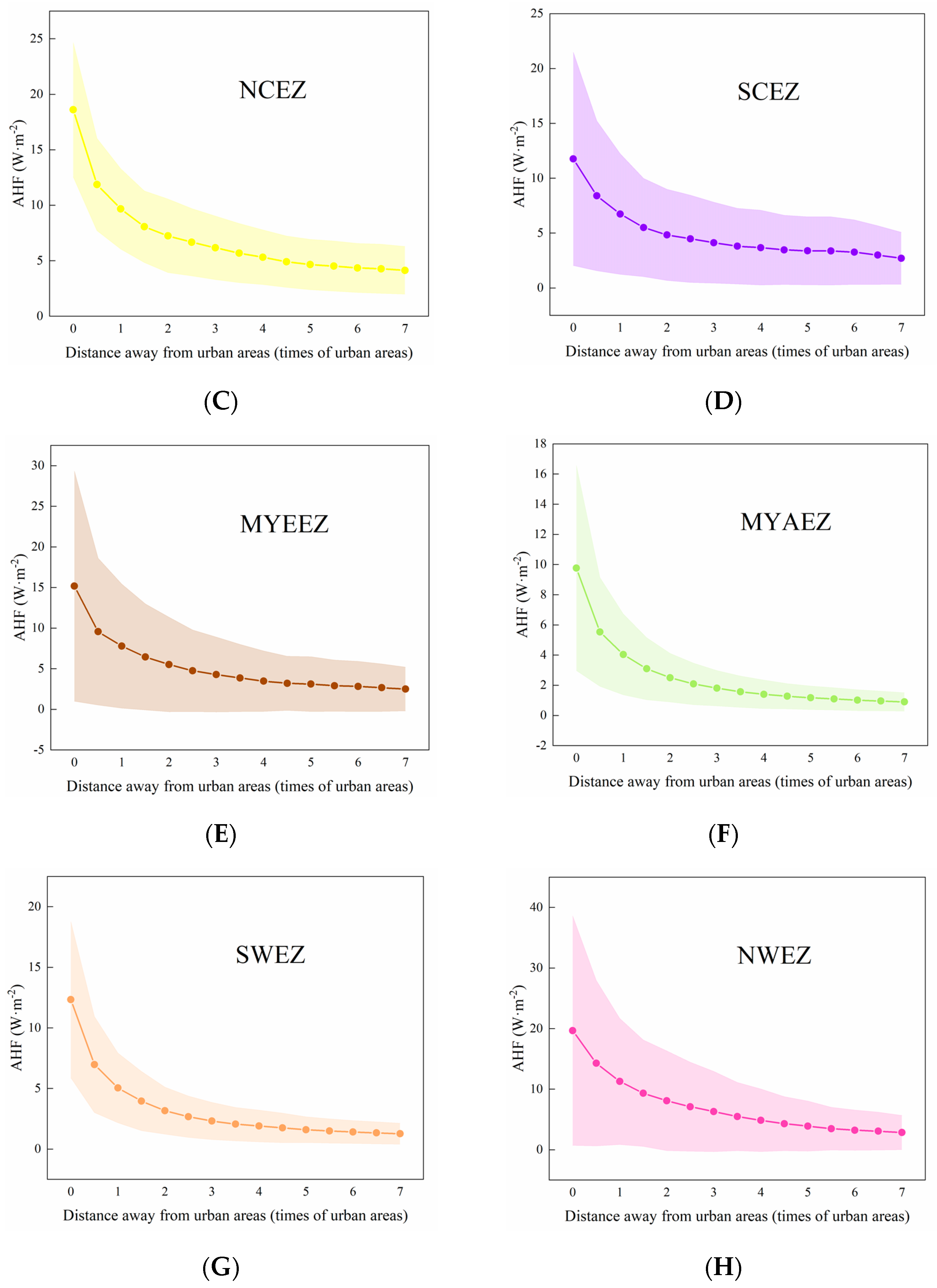
3.2. The Influence of City Sizes and Economic Zones on the Exponential Decay of ΔAHF
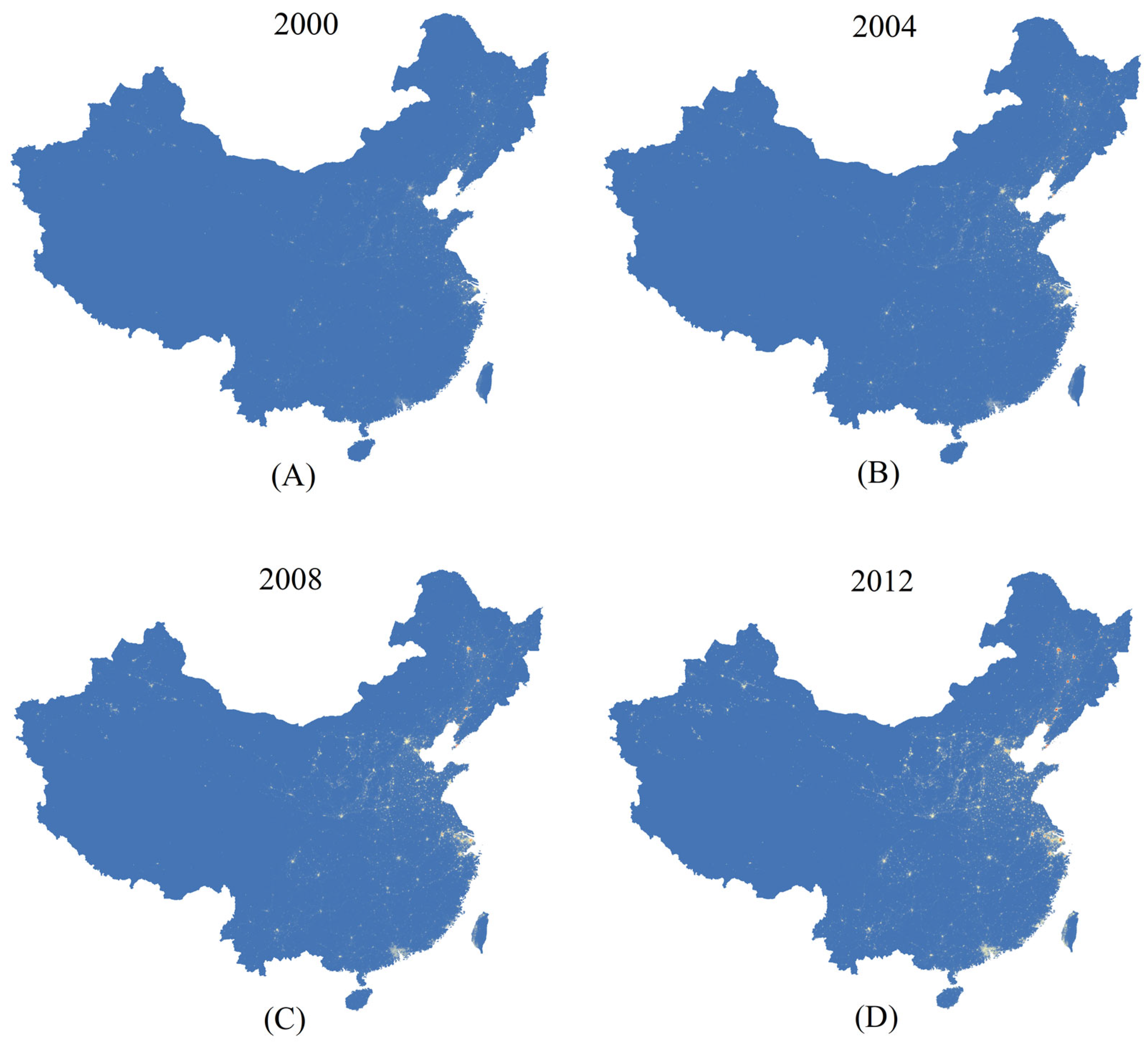
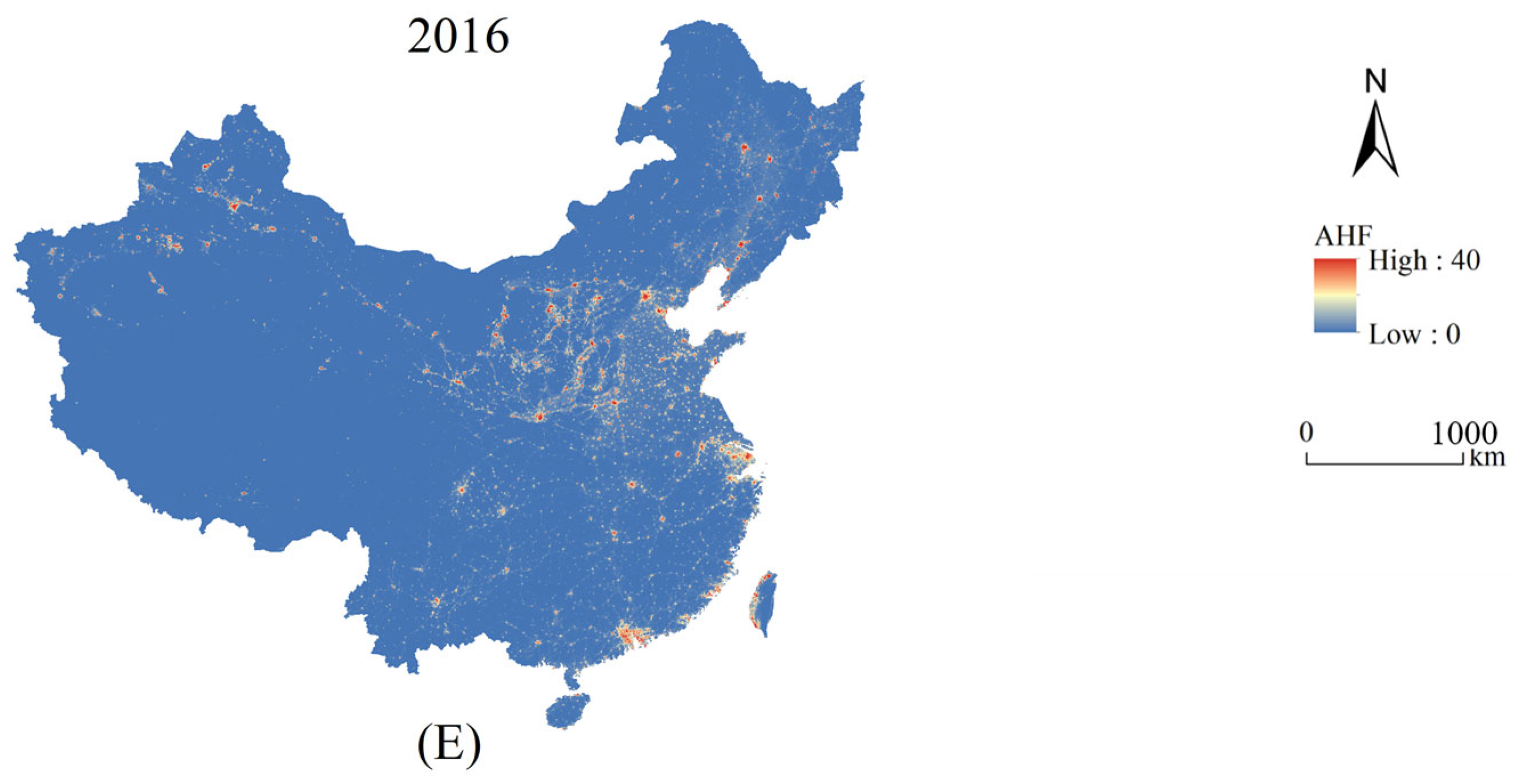
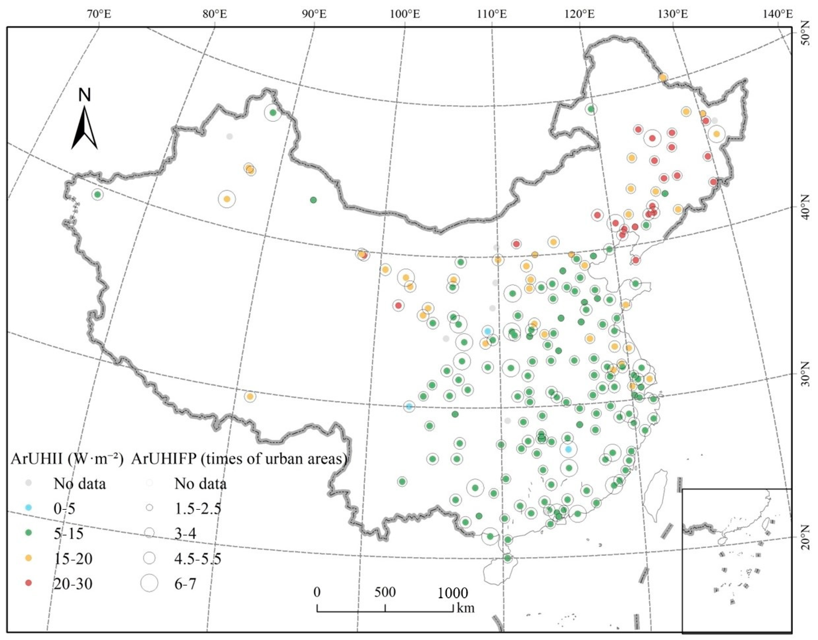
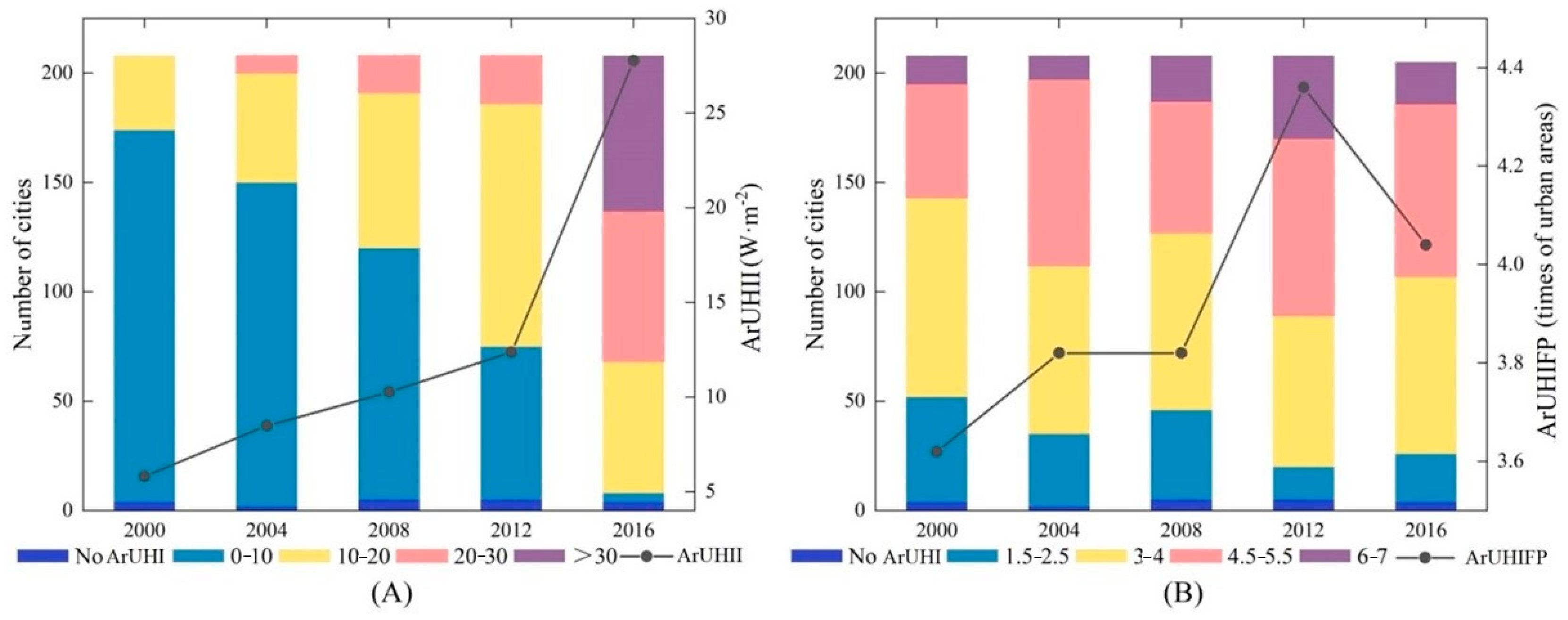
3.3. Spatiotemporal Variability in the ArUHII and ArUHIFP
4. Discussion
4.1. The Existence of ArUHIs and Correlations with Land Uses and Building Form Parameters
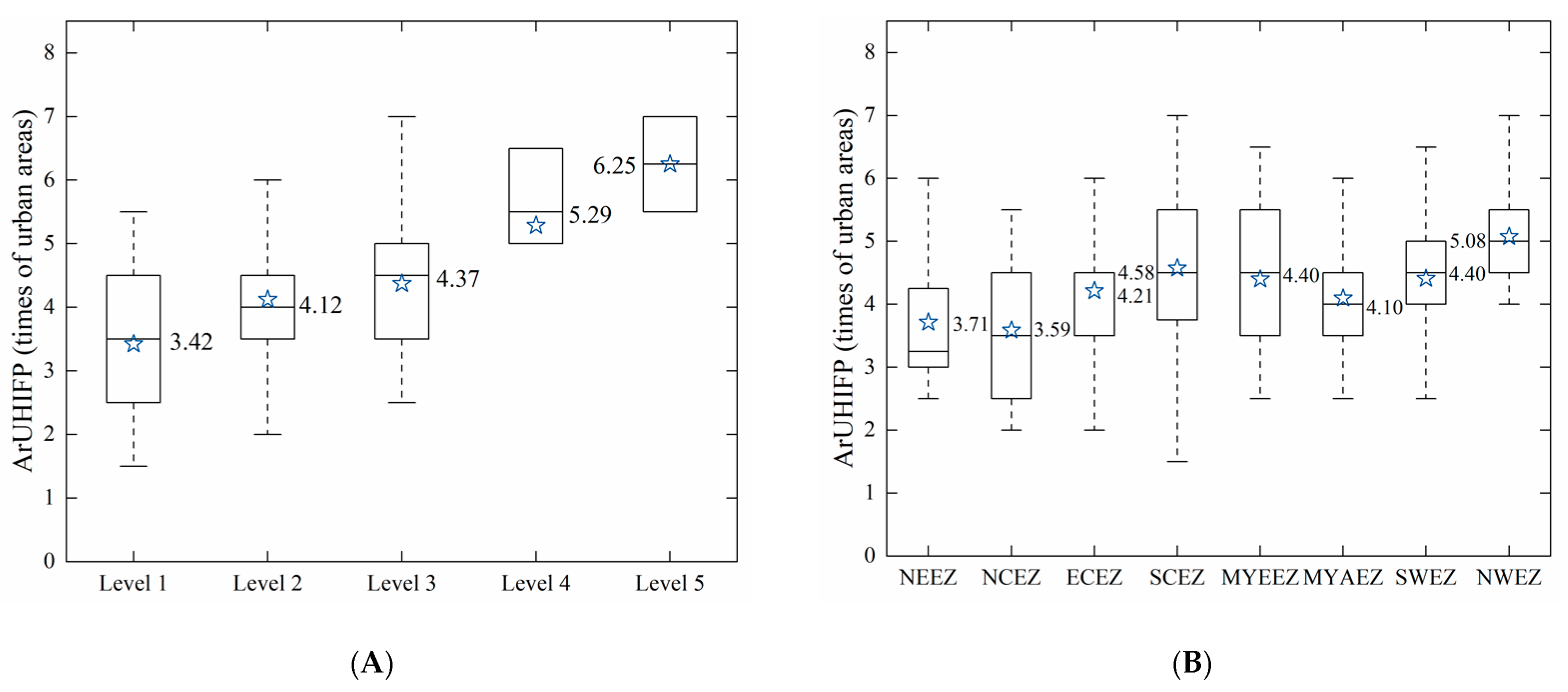
4.2. The Influence of City Sizes and Economic Zones on the ArUHIFP
4.3. The Significance of the ArUHII and ArUHIFP
5. Conclusions
Supplementary Materials
Author Contributions
Funding
Data Availability Statement
Conflicts of Interest
Nomenclature
| Nomenclature | Definition |
| Δ | Urban–rural difference |
| ΔAHF | Discrepancies in AHF between urban and rural areas |
| A | The maximum difference in AHF |
| AHE | Anthropogenic heat emission |
| AHF | Anthropogenic heat flux |
| AHF0 | AHF in urban areas |
| AHFa | The asymptotic value of the exponential trend |
| AHFb | Natural background AHF |
| AUHI | Anthropogenic urban heat island |
| AUHII | Anthropogenic urban heat island intensity |
| AUHIFP | Anthropogenic urban heat island footprint |
| BC | Building coverage |
| BFP | Building form parameter |
| CAUHI | The rate of growth of AHF between urban and rural areas |
| ECEZ | Eastern Coastal Economic Zone |
| Forest_P | The percentage of forest |
| Grass_P | The percentage of grassland |
| i | The distance from the urban area |
| MBH | Mean building height |
| MBV | Mean building volume |
| MYAEZ | Middle Yangtze River Economic Zone |
| MYEEZ | Middle Yellow River Economic Zone |
| NCEZ | Northern Coastal Economic Zone |
| NEEZ | Northeast Economic Zone |
| NWEZ | Northwest Economic Zone |
| OC_P | The percentage of other construction |
| R2 | The coefficient of determination |
| RA_P | The percentage of rural residential areas |
| RESDC | Resource and Environmental Science and Data Center |
| S | The decay rate of exponential trend |
| SCEZ | Southern Coastal Economic Zone |
| SUHI | Surface urban heat island |
| SWEZ | Southwest Economic Zone |
| WB_P | The percentage of water bodies |
References
- Sailor, D.J.; Georgescu, M.; Milne, J.M.; Hart, M.A. Development of a national anthropogenic heating database with an extrapolation for international cities. Atmos. Environ. 2015, 118, 7–18. [Google Scholar] [CrossRef]
- Ao, X.; Qian, J.; Lu, Y.; Yang, X. Mapping fine-scale anthropogenic heat flux in Shanghai by integrating multi-source geospatial big data using Cubist. Sustain. Cities Soc. 2024, 101, 105125. [Google Scholar] [CrossRef]
- Bhatt, M.M.; Gupta, K.; Danodia, A.; Chakroborty, S.D.; Patel, N. Detailed urban roughness parametrization for anthropogenic heat flux estimation using earth observation data. Heliyon 2023, 9, e18361. [Google Scholar] [CrossRef] [PubMed]
- Chen, B.; Wu, C.; Song, X.; Zheng, Y.; Lu, M.; Yang, H.; Wu, X.; Zhao, X.; Lu, Z.; Luo, T.; et al. Anthropogenic heat release due to energy consumption exacerbates European summer extreme high temperature. Clim. Dyn. 2023, 61, 3831–3843. [Google Scholar] [CrossRef]
- Huang, J.; Yue, S.; Wang, S.; Ji, G.; Cheng, M.; Li, L. Spatiotemporal Variation Characteristics Analysis of Anthropogenic Heat Fluxes Based on Nighttime Lighting Data. Pol. J. Environ. Stud. 2024, 33, 3183–3192. [Google Scholar] [CrossRef]
- Gao, L.; Yue, X.; Meng, X.; Li, D. Comparison of Ozone and PM2.5 Concentrations over Urban, Suburban, and Background Sites in China. Adv. Atmos. Sci. 2020, 37, 1297–1309. [Google Scholar] [CrossRef]
- Huang, X.; Cai, Y.; Li, J. Evidence of the mitigated urban particulate matter island (UPI) effect in China during 2000-2015. Sci. Total Environ. 2019, 660, 1327–1337. [Google Scholar] [CrossRef] [PubMed]
- Yao, L.; Sun, S.; Wang, Y.; Song, C.; Xu, Y. New insight into the urban PM2.5 pollution island effect enabled by the Gaussian surface fitting model: A case study in a mega urban agglomeration region of China. Int. J. Appl. Earth Obs. Geoinf. 2022, 113, 102982. [Google Scholar] [CrossRef]
- Hu, C.; Fung, K.Y.; Tam, C.; Wang, Z. Urbanization Impacts on Pearl River Delta Extreme Rainfall Sensitivity to Land Cover Change Versus Anthropogenic Heat. Earth Space Sci. 2021, 8, 3. [Google Scholar] [CrossRef]
- Nie, W.; Zaitchik, B.F.; Ni, G.; Sun, T. Impacts of anthropogenic heat on summertime rainfall in Beijing. J. Hydrometeorol. 2017, 18, 693–712. [Google Scholar] [CrossRef]
- Silva, R.; Carvalho, A.C.; Pereira, S.C.; Carvalho, D.; Rocha, A. Lisbon urban heat island in future urban and climate scenarios. Urban Clim. 2022, 44, 101218. [Google Scholar] [CrossRef]
- Wang, J.; Chen, Y.; Liao, W.; He, G.; Tett, S.F.B.; Yan, Z.; Zhai, P.; Feng, J.; Ma, W.; Huang, C.; et al. Anthropogenic emissions and urbanization increase risk of compound hot extremes in cities. Nat. Clim. Change 2021, 11, 1084–1089. [Google Scholar] [CrossRef]
- He, L.; Li, Q.; Wang, Y.; Lee, J.H.W.; Xu, Y.; Li, G. Effects of Urban Expansion and Anthropogenic Heat Enhancement on Tropical Cyclone Precipitation in the Greater Bay Area of China. J. Geophys. Res. Atmos. 2023, 128, e2022JD038184. [Google Scholar] [CrossRef]
- Ma, X.; Yang, B.; Dai, G.; Lin, H.; Yang, X.; Qian, Y.; Zhang, Y.; Huang, A. Contrasting Effects of Urban Land Cover Change and Anthropogenic Heat on Summer Precipitation Over the Yangtze River Delta of China: Analyses from an Atmospheric Moisture Budget Perspective. J. Geophys. Res. Atmos. 2024, 129, e2023JD039430. [Google Scholar] [CrossRef]
- Cong, J.; Wang, L.-B.; Liu, F.-J.; Qian, Z.; McMillin, S.E.; Vaughn, M.G.; Song, Y.; Wang, S.; Chen, S.; Xiong, S.; et al. Associations between metabolic syndrome and anthropogenic heat emissions in northeastern China. Environ. Res. 2022, 204, 111974. [Google Scholar] [CrossRef]
- Zeng, P.; Sun, F.; Shi, D.; Liu, Y.; Zhang, R.; Tian, T.; Che, Y. Integrating anthropogenic heat emissions and cooling accessibility to explore environmental justice in heat-related health risks in Shanghai, China. Landsc. Urban Plan. 2022, 226, 104490. [Google Scholar] [CrossRef]
- Zhang, H.-Z.; Wang, D.-S.; Wu, S.-H.; Huang, G.-F.; Chen, D.-H.; Ma, H.-M.; Zhang, Y.-T.; Guo, L.-H.; Lin, L.-Z.; Gui, Z.-H.; et al. The association between childhood adiposity in northeast China and anthropogenic heat flux: A new insight into the comprehensive impact of human activities. Int. J. Hyg. Environ. Health 2023, 254. [Google Scholar] [CrossRef] [PubMed]
- Bourne, L. Reurbanization, uneven urban development, and the debate on new urban forms. Urban Geogr. 1996, 17, 690–713. [Google Scholar] [CrossRef]
- Rubel, F.; Kottek, M. Observed and projected climate shifts 1901–2100 depicted by world maps of the Köppen-Geiger climate classification. Meteorol. Z. 2010, 19, 135–141. [Google Scholar] [CrossRef]
- He, C.; Zhou, L.; Yao, Y.; Ma, W.; Kinney, P.L. Estimating spatial effects of anthropogenic heat emissions upon the urban thermal environment in an urban agglomeration area in East China. Sustain. Cities Soc. 2020, 57, 102046. [Google Scholar] [CrossRef]
- Wang, S.; Hu, D.; Chen, S.; Yu, C. A Partition Modeling for Anthropogenic Heat Flux Mapping in China. Remote Sens. 2019, 11, 1132. [Google Scholar] [CrossRef]
- Wang, S.; Hu, D.; Yu, C.; Wang, Y.; Chen, S. Global mapping of surface 500-m anthropogenic heat flux supported by multi-source data. Urban Clim. 2022, 43, 101175. [Google Scholar] [CrossRef]
- Chen, S.; Hu, D. Parameterizing Anthropogenic Heat Flux with an Energy-Consumption Inventory and Multi-Source Remote Sensing Data. Remote Sens. 2017, 9, 11. [Google Scholar] [CrossRef]
- Liu, X.; Yue, W.; Zhou, Y.; Liu, Y.; Xiong, C.; Li, Q. Estimating multi-temporal anthropogenic heat flux based on the top-down method and temporal downscaling methods in Beijing, China. Resour. Conserv. Recycl. 2021, 172, 105682. [Google Scholar] [CrossRef]
- Wang, Y.; Hu, D.; Yu, C.; Di, Y.; Wang, S.; Liu, M. Appraising regional anthropogenic heat flux using high spatial resolution NTL and POI data: A case study in the Beijing-Tianjin-Hebei region, China. Environ. Pollut. 2022, 292, 118359. [Google Scholar] [CrossRef]
- Chen, Q.; Yang, X.; Ouyang, Z.; Zhao, N.; Jiang, Q.; Ye, T.; Qi, J.; Yue, W. Estimation of anthropogenic heat emissions in China using Cubist with Points-of-Interest and multisource remote sensing data. Environ. Pollut. 2020, 266, 115183. [Google Scholar] [CrossRef] [PubMed]
- Wang, S.; Hu, D.; Yu, C.; Chen, S.; Di, Y. Mapping China’s time-series anthropogenic heat flux with inventory method and multi-source remotely sensed data. Sci. Total Environ. 2020, 734, 139457. [Google Scholar] [CrossRef] [PubMed]
- Ming, Y.; Liu, Y.; Liu, X. Spatial pattern of anthropogenic heat flux in monocentric and polycentric cities: The case of Chengdu and Chongqing. Sustain. Cities Soc. 2022, 78, 103628. [Google Scholar] [CrossRef]
- Zhang, G.; Luo, Y.; Zhu, S. Estimation of the Spatio-Temporal Characteristics of Anthropogenic Heat Emission in the Qinhuai District of Nanjing Using the Inventory Survey Method. Asia-Pac. J. Atmos. Sci. 2019, 56, 367–380. [Google Scholar] [CrossRef]
- Liu, X.; Zhou, Y.; Yue, W.; Li, X.; Liu, Y.; Lu, D. Spatiotemporal patterns of summer urban heat island in Beijing, China using an improved land surface temperature. J. Clean. Prod. 2020, 257, 120529. [Google Scholar] [CrossRef]
- McDonald, R.; Kroeger, T.; Boucher, T.; Wang, L.; Salem, R. Planting Healthy Air: A Global Analysis of the Role of Urban Trees in Addressing Particulate Matter Pollution and Extreme Heat; The Nature Conservancy: Arlington, VA, USA, 2016. [Google Scholar]
- Heiple, S.; Sailor, D.J. Using building energy simulation and geospatial modeling techniques to determine high resolution building sector energy consumption profiles. Energy Build. 2008, 40, 1426–1436. [Google Scholar] [CrossRef]
- Han, G.; Xu, J. Land surface phenology and land surface temperature changes along an urban-rural gradient in Yangtze River Delta. Environ. Manag. 2013, 52, 234–249. [Google Scholar] [CrossRef] [PubMed]
- Imhoff, M.L.; Zhang, P.; Wolfe, R.E.; Bounoua, L. Remote sensing of the urban heat island effect across biomes in the continental USA. Remote Sens. Environ. 2010, 114, 504–513. [Google Scholar] [CrossRef]
- Zhang, X.; Friedl, M.A.; Schaaf, C.B.; Strahler, A.H.; Schneider, A. The footprint of urban climates on vegetation phenology. Geophys. Res. Lett. 2004, 31, 179–206. [Google Scholar] [CrossRef]
- Miao, Y.; Hu, X.M.; Liu, S.; Qian, T.; Xue, M.; Zheng, Y.; Wang, S. Seasonal variation of local atmospheric circulations and boundary layer structure in the Beijing-Tianjin-Hebei region and implications for air quality. J. Adv. Model. Earth Syst. 2015, 7, 1602–1626. [Google Scholar] [CrossRef]
- Chen, B.; Wu, C.; Liu, X.; Chen, L.; Wu, J.; Yang, H.; Luo, T.; Wu, X.; Jiang, Y.; Jiang, L.; et al. Seasonal climatic effects and feedbacks of anthropogenic heat release due to global energy consumption with CAM5. Clim. Dyn. 2018, 52, 6377–6390. [Google Scholar] [CrossRef]
- Kuang, H.; Hu, D.; Guo, B. Mapping regional high-resolution anthropogenic heat flux with downscaled nighttime light data. IEEE Trans. Geosci. Remote Sens. 2022, 60, 1–16. [Google Scholar] [CrossRef]
- Lin, Z.; Xu, H. Anthropogenic Heat Flux Estimation Based on Luojia 1-01 New Nighttime Light Data: A Case Study of Jiangsu Province, China. Remote Sens. 2020, 12, 3707. [Google Scholar] [CrossRef]
- Qian, J.; Meng, Q.; Zhang, L.; Hu, D.; Hu, X.; Liu, W. Improved anthropogenic heat flux model for fine spatiotemporal information in Southeast China. Environ. Pollut. 2022, 299, 118917. [Google Scholar] [CrossRef] [PubMed]
- Li, M.; Koks, E.; Taubenböck, H.; van Vliet, J. Continental-scale mapping and analysis of 3D building structure. Remote Sens. Environ. 2020, 245, 111859. [Google Scholar] [CrossRef]
- Niu, L.; Tang, R.; Jiang, Y.; Zhou, X. Spatiotemporal Patterns and Drivers of the Surface Urban Heat Island in 36 Major Cities in China: A Comparison of Two Different Methods for Delineathing Rural Areas. Sustainability 2020, 12, 478. [Google Scholar] [CrossRef]
- Fu, P.; Weng, Q. Variability in Annual Temperature Cycle in the Urban Areas of the United States as Revealed by MODIS Imagery. ISPRS J. Photogramm. Remote Sens. 2018, 146, 65–73. [Google Scholar] [CrossRef]
- Zhou, D.; Zhang, L.; Hao, L.; Sun, G.; Liu, Y.; Zhu, C. Spatiotemporal trends of urban heat island effect along the urban development intensity gradient in China. Sci. Total Environ. 2016, 544, 617–626. [Google Scholar] [CrossRef]
- Zhou, D.; Zhao, S.; Zhang, L.; Sun, G.; Liu, Y. The footprint of urban heat island effect in China. Sci. Rep. 2015, 5, 11160. [Google Scholar] [CrossRef] [PubMed]
- Yu, C.; Hu, D.; Wang, S.; Chen, S.; Wang, Y. Estimation of anthropogenic heat flux and its coupling analysis with urban building characteristics—A case study of typical cities in the Yangtze River Delta, China. Sci. Total Environ. 2021, 774, 145805. [Google Scholar] [CrossRef]
- Horrace, W.C.; Oaxaca, R.L. Results on the bias and inconsistency of ordinary least squares for the linear probability model. Econ. Lett. 2006, 90, 321–327. [Google Scholar] [CrossRef]
- Cabral, P.; Santos, J.A.; Augusto, G. Monitoring urban sprawl and the national ecological reserve in Sintra-Cascais, Portugal: Multiple OLS linear regression model evaluation. J. Urban Plan. Dev. 2011, 137, 346–353. [Google Scholar] [CrossRef]
- Lopes, M. Chinese industrialization from the New-Developmental perspective. Braz. J. Political Econ. 2020, 40, 53–67. [Google Scholar]
- Long, C.; Zhang, X. Patterns of China’s industrialization: Concentration, specialization, and clustering. China Econ. Rev. 2012, 23, 593–612. [Google Scholar] [CrossRef]
- Singh, V.K.; Mughal, M.O.; Martilli, A.; Acero, J.A.; Ivanchev, J.; Norford, L.K. Numerical analysis of the impact of anthropogenic emissions on the urban environment of Singapore. Sci. Total Environ. 2022, 806, 150534. [Google Scholar] [CrossRef]
- Dong, Y.; Varquez, A.; Kanda, M.; Dong, Y.; Varquez, A.; Kanda, M. Global anthropogenic heat flux database with high spatial resolution. Atmos. Environ. 2017, 150, 276–294. [Google Scholar] [CrossRef]
- Peng, T.; Sun, C.; Feng, S.; Zhang, Y.; Fan, F. Temporal and Spatial Variation of Anthropogenic Heat in the Central Urban Area: A Case Study of Guangzhou, China. ISPRS Int. J. Geo-Inf. 2021, 10, 160. [Google Scholar] [CrossRef]
- Xu, X.; Liu, J.; Zhang, S.; Li, R.; Yan, C.; Wu, S. China Multi-Temporal Land Use Remote Sensing Monitoring Dataset (CNLUCC). Resour. Environ. Sci. Data Regist. Publ. Syst. 2018. [Google Scholar] [CrossRef]
- Xue, Q.; Song, W. Spatial Distribution of China’s Industrial Output Values under Global Warming Scenarios RCP4.5 and RCP8.5. ISPRS Int. J. Geo-Inf. 2020, 2020, 724. [Google Scholar] [CrossRef]
- Sun, R.; Wang, Y.; Chen, L. A distributed model for quantifying temporal-spatial patterns of anthropogenic heat based on energy consumption. J. Clean. Prod. 2018, 170, 601–609. [Google Scholar] [CrossRef]
- Wu, H.; Huang, B.; Zheng, Z.; Sun, R.; Hu, D.; Zeng, Y. Urban anthropogenic heat index derived from satellite data. Int. J. Appl. Earth Obs. Geoinf. 2023, 118, 103261. [Google Scholar] [CrossRef]


| Level | Abbreviation | Population Size |
|---|---|---|
| Super city | Level 1 | >10 million |
| Mega city | Level 2 | >3 million, and <10 million |
| Large city | Level 3 | >1 million, and <3 million |
| Medium city | Level 4 | >500,000, and <1 million |
| Small city | Level 5 | <500,000 |
| Data | Year | Resolution | Source |
|---|---|---|---|
| AHF data | 2000–2016 | 500 m × 500 m | https://doi.org/10.1016/j.scitotenv.2020.139457 (accessed on 1 August 2022) |
| Land use data | 2000–2015 | 1 km × 1 km | https://www.resdc.cn/DOI/DOI.aspx?DOIID=54 (accessed on 1 August 2022) |
| 2D and 3D building form data | 2015 | 1 km × 1 km | https://doi.org/10.1016/j.rse.2020.111859 (accessed on 1 August 2022) |
| Category | Parameter | Abbreviation | Definition | Source |
|---|---|---|---|---|
| Land use patterns | Rural residential area proportion | RA_P | The percentage of rural residential area in a 1 × 1 km grid | RESDC |
| Proportion of other types of construction | OC_P | The percentage of other types of construction in a 1 × 1 km grid | RESDC | |
| Building forms | Building coverage | BC | The proportion of building area to total pixel area | Li et al. (2020) [41] |
| Mean building height | MBH | The average height of buildings | Li et al. (2020) [41] | |
| Mean building volume | MBV | The average volume of buildings | Li et al. (2020) [41] |
| Year | A | S | AHFa | R2 |
|---|---|---|---|---|
| 2000 | 5.55 ± 0.19 | 0.99 ± 0.07 | 1.00 ± 0.08 | 0.99 |
| 2004 | 8.20 ± 0.26 | 0.96 ± 0.07 | 1.42 ± 0.10 | 0.99 |
| 2008 | 9.91 ± 0.31 | 1.01 ± 0.07 | 1.97 ± 0.12 | 0.99 |
| 2012 | 11.84 ± 0.37 | 1.20 ± 0.08 | 2.99 ± 0.17 | 0.99 |
| 2016 | 26.84 ± 0.99 | 1.01 ± 0.08 | 6.08 ± 0.39 | 0.98 |
| Mean | 12.44 ± 0.43 | 1.04 ± 0.08 | 0.32 ± 0.17 | 0.99 |
| City Size | A | S | AHFa | R2 |
|---|---|---|---|---|
| L1 | 13.83 ± 0.45 | 1.33 ± 0.02 | 3.11 ± 0.15 | 0.99 |
| L2 | 13.39 ± 0.14 | 1.11 ± 0.06 | 2.34 ± 0.14 | 0.99 |
| L3 | 12.21 ± 0.42 | 0.96 ± 0.08 | 2.60 ± 0.17 | 0.98 |
| L4 | 14.45 ± 0.65 | 0.40 ± 0.02 | 2.23 ± 0.64 | 0.98 |
| L5 | 19.71 ± 0.37 | 0.49 ± 0.10 | 2.12 ± 0.29 | 0.99 |
| Economic Zone | A | S | AHFa | R2 |
|---|---|---|---|---|
| NEEZ | 21.01 ± 0.97 | 0.88 ± 0.12 | 3.23 ± 0.42 | 0.97 |
| ECEZ | 12.94 ± 0.31 | 1.27 ± 0.04 | 2.24 ± 0.11 | 0.99 |
| NCEZ | 13.26 ± 0.55 | 0.92 ± 0.10 | 4.67 ± 0.23 | 0.98 |
| SCEZ | 8.35 ± 0.22 | 0.83 ± 0.07 | 3.20 ± 0.10 | 0.99 |
| MYEEZ | 11.66 ± 0.42 | 0.82 ± 0.10 | 2.90 ± 0.19 | 0.99 |
| MYAEZ | 8.31 ± 0.27 | 1.02 ± 0.07 | 7.17 ± 0.10 | 0.99 |
| SWEZ | 10.37 ± 0.33 | 1.06 ± 0.06 | 1.61 ± 0.12 | 0.99 |
| NWEZ | 16.00 ± 0.41 | 0.58 ± 0.11 | 3.00 ± 0.27 | 0.99 |
Disclaimer/Publisher’s Note: The statements, opinions and data contained in all publications are solely those of the individual author(s) and contributor(s) and not of MDPI and/or the editor(s). MDPI and/or the editor(s) disclaim responsibility for any injury to people or property resulting from any ideas, methods, instructions or products referred to in the content. |
© 2024 by the authors. Licensee MDPI, Basel, Switzerland. This article is an open access article distributed under the terms and conditions of the Creative Commons Attribution (CC BY) license (https://creativecommons.org/licenses/by/4.0/).
Share and Cite
Cui, L.; Chen, Q. Investigating Variations in Anthropogenic Heat Flux along Urban–Rural Gradients in 208 Cities in China during 2000–2016. Buildings 2024, 14, 2766. https://doi.org/10.3390/buildings14092766
Cui L, Chen Q. Investigating Variations in Anthropogenic Heat Flux along Urban–Rural Gradients in 208 Cities in China during 2000–2016. Buildings. 2024; 14(9):2766. https://doi.org/10.3390/buildings14092766
Chicago/Turabian StyleCui, Ling, and Qiang Chen. 2024. "Investigating Variations in Anthropogenic Heat Flux along Urban–Rural Gradients in 208 Cities in China during 2000–2016" Buildings 14, no. 9: 2766. https://doi.org/10.3390/buildings14092766
APA StyleCui, L., & Chen, Q. (2024). Investigating Variations in Anthropogenic Heat Flux along Urban–Rural Gradients in 208 Cities in China during 2000–2016. Buildings, 14(9), 2766. https://doi.org/10.3390/buildings14092766