Enhancing Building Energy Efficiency Estimations Through Graph Machine Learning: A Focus on Heating and Cooling Loads

Abstract

In this paper, we introduce graph machine learning to enhance the estimation of heating and cooling loads in buildings, a critical factor in building energy efficiency. Traditional methods often overlook the complex interaction between building topology and geometric characteristics, leading to less accurate predictions. This research bridges this gap by incorporating these elements into a graph-based machine learning framework. This study introduces a parametric generative workflow to create a synthetic dataset, which is central to this research. This dataset encompasses multiple building forms, each with unique topological connections and attributes, ensuring a thorough analysis across varied building scenarios. The research involves simulating diverse building shapes and glazing scenarios with different window sizes and orientations. The study primarily utilizes Deep Graph Learning (DGL) for training, with Random Forest (RF) serving as a baseline for validation. Both DGL and RF algorithms demonstrate high performance in predicting heating and cooling loads.

1. Introduction

Buildings are significant contributors to overall energy consumption. With the advancement of machine learning techniques, there is growing interest in exploring their potential to reduce building energy use and improve the accuracy of load estimation. Common machine learning methods applied to building energy prediction include support vector machines (SVMs) and artificial neural networks (ANNs).

Support vector machines (SVMs) are employed for predicting building energy consumption with limited samples, using structural risk minimization. Zhong et al. enhanced prediction accuracy by optimizing feature space through support vector regression [1]. Dong et al. applied SVMs to predict tropical commercial building energy consumption, yielding small prediction errors due to a modest data pool [2]. However, SVM’s suitability for non-linear high-dimensional patterns is offset by memory and computational demands, posing challenges for large-scale training samples.

Artificial neural networks (ANNs) are favored for accurate building energy consumption predictions due to self-learning and robust non-linear function fitting capabilities. Research highlights ANNs’ superiority; Wei et al. utilized a feed-forward neural network for office building occupancy and energy forecasts, Ekici and Aksoy employed backpropagation for heating energy estimations, and Rahman introduced a recurrent neural network for extended-term power predictions [3,4,5]. However, shallow neural networks risk data loss and rely on trial-and-error network topology selection, challenging the attainment of an optimal configuration.

Traditional machine learning (ML) methods typically treat data as flat tables, where each row is an independent example, and each column (or feature) is assumed to contribute equally. Traditional ML typically require fixed-size input vectors and struggle with this variability. However, many real-world problems involve elements that are interconnected and of diverse sizes. Graph machine learning (GML) addresses this by representing data as a graph made up of nodes (entities) and edges (relationships between entities). By learning from both the attributes of the nodes and the way they are connected, GML can uncover patterns that traditional ML approaches often miss, particularly in complex systems with relational dependencies. This is particularly valuable in fields like architecture, engineering, and construction (AEC), where the relationships between entities are just as important as the entities themselves. Unlike traditional ML models, GML incorporates the topology of the data, leveraging information such as node degrees, connectivity patterns, and regional structures within the graph. This allows for a more accurate representation and analysis of structured data which enhances the predictive performance of applications like building energy efficiency estimations. Additionally, GML is ideal for applications with significant variations in data size and shape, as graphs often exhibit different numbers of nodes and edges.

This study aims to investigate the effectiveness of graph machine learning approaches in estimating heating and cooling loads by leveraging a combination of topological and geometric attributes. Heating and cooling loads are fundamental indicators of a building’s energy demand for maintaining optimal indoor conditions. Precise estimation of these loads requires a comprehensive understanding of the intricate interplay between a building’s spatial layout (topology) and its physical attributes (geometric features).

The novelty of this study lies in applying sophisticated graph machine learning (GML) to estimate heating and cooling loads by explicitly incorporating building topology alongside geometry, which is an approach not explored in prior literature. We further contribute a reproducible generative modeling workflow and conduct comparative evaluation of GML against other ML models, such as Random Forest. This study highlights the advantages of using GML over traditional batch simulations in predicting building heating and cooling loads. While based on simulation-generated data, the study serves as a foundation for developing methodologies that can later be applied to real-world data. The synthetic dataset allows for controlled testing and model optimization, ensuring scalability for future real-world applications.

Applying GML to building energy analysis requires a fundamental shift in how buildings, spaces, and their components are represented. Unlike traditional data formats, GML must meaningfully capture the building’s spatial and functional organization. The effectiveness of GML depends on the underlying graph structure, as well as on the careful selection and encoding of node and edge attributes such as surface area, orientation, material properties, and usage type, all of which influence energy behavior. Designing such representations involves deliberate abstraction and domain-specific knowledge to ensure that both topology and geometry are accurately embedded into the graph, enabling the model to learn relevant patterns and relationships that drive heating and cooling demands.

To achieve the stated aim, the research pursued several objectives: firstly, we created a parametric generative workflow closely following the precedent set by [6]. We generated an identical number of building forms, with identical glazing ratios and orientations. We then diversified this dataset with distinct topological connections and information. Repeating Chou and Bui’s generative workflow ensures research reproducibility and verifies their results under similar conditions. This was followed by conducting sensitivity analysis to identify the optimal combination of topological, geometrical, and informational attributes to include in the dataset. Additionally, a random search was performed to optimize hyper-parameters. Lastly, several machine learning models were tested and compared to determine their effectiveness. By introducing graph machine learning and validating our results through a Random Forest model, we were able to explore the generalizability and potential of alternative methodologies to enable a broader understanding of predictive tools for building energy loads.

The research design for this study includes four main steps. Firstly, a sample of various building shapes is created to ensure a diverse range of shapes. Next, different scenarios for glazing are created by varying the size and direction of the windows as well as their percentages for each compass direction. These scenarios are then analyzed using thermal simulation techniques to create the dataset for ML use. Lastly, the results from the simulations, such as cooling and heating load indexes, are used to train the Deep Graph Learning (DGL) and Random Forest Algorithm (RFA) model to predict energy consumption.

The subsequent sections of this paper are structured as follows: The ensuing section introduces the study’s context by delving into relevant literature, encompassing investigations into energy performance of buildings (EPB) and predictive methodologies. Section 3 details the research methodology employed as well as the methods employed for evaluation. In Section 4, an account is provided of the building information and experimental data obtained for this study. The modeling processes are outlined in Section 5, wherein prediction outcomes are discussed, and a comparison of model performance is offered. The paper concludes with reflections and an account of the contributions made by this research in the closing section.

2. Related Work

2.1. Building Energy Simulation (BES)

Building performance simulation is a prominent and evolving field, encompassing automated design, energy modeling, predictive control, digital twins, and demand response solutions. These advancements hold potential for reducing CO₂ emissions, enhancing building quality and user experiences, and increasing productivity in construction and maintenance. Building performance simulation is crucial for the architectural industry’s future development.

Y. Pan et al. 2023 primarily discusses the research directions and status of building energy modeling (BEM) over the past decade [7]. It also outlines future challenges, focusing on acquiring high-quality data, efficient modeling algorithms, workflow intelligence, and large-scale urban simulations. Researchers aim to address these challenges in various BEM application scenarios [7].

Gonzalo 2023 compared various building energy simulation (BES) tools modeling an office cell in Boston, USA, and Madrid, Spain, assessing heating and cooling loads on yearly, monthly, and hourly bases [8]. It classified tools into basic online tools, general-purpose engines (e.g., TRNSYS, IDA ICE), and special-purpose tools (e.g., EnergyPlus). The research used cross-validation and statistical analysis to evaluate the reliability of simulations. While yearly heating and cooling demand had minor deviations (0.1% to 5.3%), monthly deviations ranged from 10% to 20%. However, hourly energy demand analysis showed significant errors (35% to 50%), highlighting the need for improved accuracy in hourly predictions [8].

Harishn et al. 2016, highlights various modeling methodologies for building energy systems, with a focus on methodologies that enable control strategy development [9]. Models are categorized by their approach, and available simulation programs and software are discussed. These efforts aim to create computationally efficient models to enhance energy conservation and efficiency in buildings [9].

A study by Subrammania et al. 2018 examines the modeling and simulation of energy systems, a critical driver of the modern economy [10]. It proposes two categorization methods: one based on modeling approaches (computational, mathematical, physical, or hybrid models) and another based on fields (Process Systems Engineering—PSE and Energy Economics—EE). By comparing variables, theoretical foundations, aggregation levels, spatial-temporal scales, and model objectives, the differences between PSE, which traditionally focuses on technological aspects, and EE, which considers broader economic contexts, are highlighted. The study advocates combining these approaches for a more comprehensive understanding of energy systems within economic and policy contexts, illustrating its value through three application areas: optimal process design, sustainability analysis, and handling feedback effects of innovative technologies [10].

2.2. Simplified Topology

Simplified topology in architecture refers to the use of streamlined geometric and spatial configurations in architecture. This approach focuses on reducing complexity in the building’s structure and layout, emphasizing efficiency, ease of construction, and clarity in form and function. Simplified topology is often employed to achieve esthetic minimalism and cost-effectiveness, while also considering the practical aspects of space utilization and building performance. This strategy aligns with contemporary trends towards sustainability and functional simplicity in architecture. This idea firstly introduced by Robert Aish and Wassim Jabi which lead to the creation of a tool called Topologic [11,12]. Jabi’s (2015, 2016) work explored non-manifold topology (NMT) for early-stage 3D modeling in building design, aiming for compatibility with building performance simulation (BPS) inputs without simplifying BIM-generated polyhedral models. The research involved software and library evaluation, design criteria review, software prototype development, and case study analysis. Findings indicate NMT’s effectiveness in representing buildings for BPS engines, offering architects a topological design approach with early performance insights using simple 3D models [13,14].

Chatzivasileiadi et al. (2018a) investigated three methods for energy modeling of a standard office building test case using EnergyPlus [15]. These methods included: (a) OpenStudio using Topologic’s NMT system, (b) OpenStudio using the SketchUp 3D modeling tool and (c) through the DesignBuilder graphical interface. The Topologic NMT pathway excelled in handling complex geometries and provided reliable results, showcasing NMT’s spatial representation benefits and curved geometry idealization for energy simulations [15].

2.3. Machine Learning for Energy Analysis

2.3.1. Convolutional Neural Network (CNN)

In 2003, Werner and Mahdavi explored the reliability of simple geometric compactness indicators used in energy-related building standards. These indicators rely on the relationship between a building’s volume and surface area to assess thermal insulation criteria. The study uses parametric thermal simulations to investigate the accuracy of these indicators in evaluating energy-related assessments. It examines how buildings with the same compactness attribute can vary in terms of enclosure transparency, orientation, and morphology, highlighting the potential limitations of using such indicators alone [16].

Tsanas and Xifara 2012, presents a statistical machine learning framework for analyzing the impact of eight input variables on two output variables in residential buildings: heating load and cooling load [17]. The authors use classical and non-parametric statistical analysis tools to evaluate the relationship between each input variable and the output variables. They compare a linear regression approach to a non-linear non-parametric method called Random Forests for estimating the heating and cooling loads. Simulations on 768 residential buildings demonstrated that the framework can accurately predict the loads with low mean absolute error deviations from ground truth values established using Ecotect. The study supports the use of machine learning tools for estimating building parameters as a convenient and accurate approach, if the query is similar to the data used to train the model [17].

Chou and Bui in 2014, presented a study on estimating the energy performance of buildings using various data mining techniques. The authors compared several models such as support vector regression (SVR), artificial neural network (ANN), classification and regression tree, chi-squared automatic interaction detector, general linear regression, and ensemble inference model. The models were constructed using 768 experimental datasets from literature, with 8 input parameters and 2 output parameters (cooling load and heating load). The comparison results revealed that the ensemble approach (SVR + ANN) and SVR were the most accurate models for predicting cooling load and heating load, respectively, with mean absolute percentage errors below 4%. Additionally, the ensemble model and SVR model outperformed previous works by achieving at least 39.0% to 65.9% lower Root Mean Square Errors for cooling load and heating load prediction. This study highlights the efficiency, effectiveness, and accuracy of the proposed approach in predicting cooling load and heating load during the building design stage. The results demonstrate the feasibility of using these techniques to facilitate early designs of energy-conserving buildings [6].

Moayedi et al. 2019, evaluates six machine learning techniques for heating load calculation in energy-efficient building design, as part of the HVAC system design process [18]. The methods include multi-layer perceptron regressor (MLPr), Lazy Locally Weighted Learning (LLWL), Alternating Model Tree (AMT), Random Forest (RF), ElasticNet (ENet), and Radial Basis Function Regression (RBFr). These models were assessed using statistical indices such as RRSE, RMSE, MAE, R², and RAE. The Random Forest (RF) model was found to be the most effective, demonstrating superior accuracy in predicting heating loads in energy-efficient buildings, based on its high performance in both training and testing datasets [18].

Recently Yan et al. 2023, focused on the prediction and analysis of cooling and heating loads in residential buildings as a measure of energy efficiency [19]. The authors used a multi-layer perceptron neural network to predict these loads based on an experimental dataset that considers the impact of building dimensions on energy consumption. To optimize the training process of the neural network, various optimizers were used and compared in terms of accuracy and authenticity. The findings highlight the excellent performance of the adaptive chaotic gray wolf optimization method, which achieves the highest accuracy in forecasting energy consumption. The hybrid approach combining the multi-layer perceptron neural network and adaptive chaotic gray wolf optimization is found to be the most effective. The optimal number of neurons in the hidden layer is determined to be 15. The selected method achieves an R² of 0.9123 and 0.9419 for cooling and heating loads, respectively, as per the statistical performance indicators [19].

Although much work has been performed in the field, no research has yet investigated how graph machine learning approaches can accurately estimate heating and cooling loads by leveraging a combination of topology and geometric attributes.

2.3.2. Random Forest (RF) and Decision Trees (DT)

Random Forest combines multiple decision trees to produce a more accurate and stable prediction. In ensemble learning, multiple models are used to solve the same problem and then aggregated to improve the overall performance. Ahmad et al. 2017 [20], described the fundamental attributes of the Random Forest algorithm as follows: Firstly, it employs bootstrap resampling, a technique that involves random sampling with replacement. Secondly, the algorithm utilizes random selection of features for decision-making in the model. Lastly, it is characterized by the development of decision trees to their full depth, ensuring a comprehensive growth of each tree in the forest [21].

The decision tree (DT) technique, widely employed in various domains for classification and prediction [22], employs a tree-like structure to partition datasets into predefined classes, offering categorization, description, and data generalization [19]. The ease of use and efficient predictive capabilities with minimal computation time make the DT model advantageous compared to other models. Although capable of handling both numerical and categorical data, DT tends to excel more with categorical data than numerical counterparts [22]. In the context of building studies, some applications have utilized DT techniques. Tso and Yau (2006) conducted a comparative analysis of three modeling approaches to predict average weekly electricity consumption in Hong Kong [22]. The study revealed that DT-applicable models outperformed regression models due to their capacity to grasp energy consumption patterns and accurately predict energy usage. In a separate investigation a predictive model was formulated to enhance building energy efficiency through DT utilization [23]. Employing DT techniques on a residential structure, they forecasted energy use intensity (EUI) levels. The findings indicated that the DT method enabled precise classification and prediction of building energy usage, thus promoting high energy-performance buildings.

Alammar et al. 2021, introduces an innovative approach to efficiently assess solar radiation intensity on office building envelopes using machine learning models, specifically artificial neural network (ANN) and decision tree (DT) [24]. A generative parametric office tower and urban context were simulated to create a synthetic dataset. The comparison of the two machine learning models indicated that decision tree (DT) outperformed artificial neural network (ANN) due to the mostly categorical nature of the data, aligning well with DT algorithms [24].

Alammar et al. 2023, explores the use of a decision tree (DT) model as an alternative and efficient method to predict hourly cooling loads for adaptive façades in comparison to traditional building performance simulation (BPS) [25]. Using generative parametric modeling and synthetic datasets, the DT model demonstrated high accuracy in estimating cooling loads within seconds. The findings suggest that decision tree surrogate models can be valuable tools for researchers and designers in assessing adaptive façade designs, offering substantial time savings and computational efficiency [25].

3. Graph Theory and Applications of Graph Convolutional Neural Networks (DGCNN)

Graph theory is a powerful tool for describing and analyzing connections between objects. In graph theory, relationships are represented and studied using graphs, which originate in mathematics but also extend into other fields. Graph theory facilitates the representation and analysis of connections between two objects in a versatile and comprehensive manner. Using this approach, objects are represented as nodes (or vertices) in a graph, with edges illustrating the relationships between them. The edge’s properties, like its weight and direction, shed light on the connection’s strength and nature, whether it is unidirectional or reciprocal. When these objects are part of a larger network, graph theory becomes even more crucial. It helps in understanding how changes in one node affect another, using concepts such as network flow, connectivity, and pathfinding. Beyond representing direct links, graph theory is adept at modeling complex relationships, including indirect interactions, dependencies, and hierarchical structures. Its ability to provide a visual and intuitive representation makes it easier to comprehend and communicate the intricacies of these connections. The application of graph theory extends across various fields, from computer science, where it is used for network and data structure analysis, to biology for studying ecosystems or neural networks, and to sociology for analyzing social networks. This broad applicability underscores its significance as a tool for understanding and interpreting complex structures.

In 2020, Jabi and Alymani introduced a novel approach to urban and architectural classification, replacing 2D images with topological graphs for machine learning [26]. The following year, Alymani and Jabi extended this idea, utilizing architectural topological models integrated with graph machine learning to analyze building-ground interactions [27]. They presented a case study illustrating these relationships, offering guidelines for creating a 3D synthetic architectural database. Their subsequent paper detailed a workflow using deep graph convolutional neural networks to classify 3D architectural prototypes based on topological graphs, yielding precise outcomes for designers selecting optimal building-ground interactions. The study emphasizes the efficacy of non-manifold topology for accurate graph-level prediction [28].

4. Methodology

This research employs a systematic approach to explore the integration of building energy analysis with advanced machine learning techniques, focusing on graph-based methods for predicting heating and cooling loads in buildings. The topological models were constructed using a combination of geometric parameters and energy simulation software, including EnergyPlus (24.1.0). These tools were employed to simulate building energy consumption under various scenarios, enabling the generation of a dataset that reflects different topologies and physical characteristics. The topological structure of the building is embedded within the dataset through the representation of nodes and edges, where nodes represent building elements (rooms, walls, apertures), and edges denote their spatial relationships. The graph’s connectivity captures how these elements interact thermally, influencing energy consumption.

4.1. Methodology Structure

The methodology is structured into several key phases; each designed to build upon the previous step and collectively contribute to achieving the research objectives (see Figure 1).

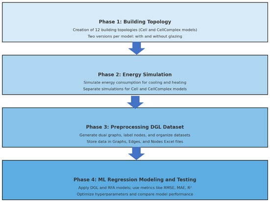
Figure 1. Methodological Structure into Several Key Phases.

Phase 1: Building Topology: involves the creation of 12 distinct building topologies with two key tasks. First, Specifying Utility Functions, where notable features for each building topology are defined, including the orientation of faces (North, South, East, West), critical for assessing sun exposure and energy efficiency. Second, Exporting Building Models, where two versions of each model are produced: one with glazing percentage, incorporating specified percentages of glazing (window area) for natural light and thermal performance considerations, and another without glazing percentage for comparative analysis of glazing’s impact on building performance and esthetics. It is important to note here that the building generator creates two parallel representations of buildings. The first representation is a simple single-zone model, which Topologic calls a Cell, while the second representation is a multi-zone cellular form which Topologic calls a CellComplex. This phase is fundamental for establishing a diverse range of building designs for subsequent analysis and development. Moreover, the 12 building forms represent a range of topological and geometric complexities, selected to cover diverse scenarios in building energy performance. Additionally, the 12 building forms closely follow the precedent set by [6], to replicate the process of data creation and compare this methodology and results with theirs.

To check the accuracy of the 3D building models created in Phase 1 within a user interface, a script was developed to enable their interactive display and exploration. This is important for verifying the models and conducting in-depth analysis and visualization of their design features (see Figure 2).

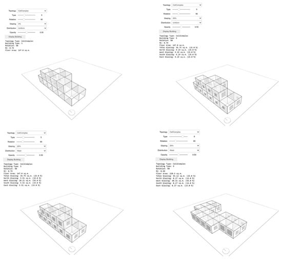
Figure 2. Building Explorer User Interface showing 3D models of generated building topologies with glazing variations for energy simulation input. Models include glazing percentages of 10%, 25%, and 40% across four orientations.

Phase 2: Energy Simulation: In this phase, energy simulations are run for both Cells and CellComplexes. For each type of model, simulations are first conducted for cooling loads, followed by simulations for heating loads.

Phase 3: Preprocessing DGL Dataset: This phase imports all the cooling and heating datasets for both the Cell and CellComplex versions of the building models. It then automatically generates dual graphs (see Figure 3), labels them, and saves the graph datasets in CSV format (see Table 1). A dual graph is a graph where each vertex represents an element of the original model, and edges connect vertices whose corresponding elements in the original graph share a boundary or a relationship. The datasets for both heating and cooling loads are organized into three Excel files as follows:

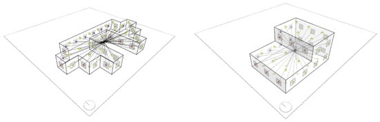
Figure 3. User interface “dual graphs”.

Table 1. The total number of graph node labels was 33 labels.

Types	Labels	Types	Labels	Types	Labels	Types	Labels	Types	Labels
Room	0	Aperture N XS	7	Aperture W XS	13	Aperture S XS	19	Aperture S XS	25
Wall N	1	Aperture N S	8	Aperture W S	14	Aperture S S	20	Aperture S S	26
Wall W	2	Aperture N M	9	Aperture W M	15	Aperture S M	21	Aperture S M	27
Wall S	3	Aperture N L	10	Aperture W L	16	Aperture S L	22	Aperture S L	28
Wall E	4	Aperture N XL	11	Aperture W XL	17	Aperture S XL	23	Aperture S XL	29
Floor	5	Aperture N XXL	12	Aperture W XL	18	Aperture S XL	24	Aperture S XL	30
Roof	6							Partitions	31
								Slabs	32

• Graphs: This Excel file includes the graph labels (its cooling or heating load) along with its number of nodes/vertices.
• Edges: This Excel file includes the edges that represent the relationships between nodes. It includes source and destination indices into the list of nodes/vertices.
• Nodes: This Excel file includes the nodes/vertices that represent the components in the building model (space, wall, ceiling, floor, aperture, etc.) along with each node’s categorical label (see Figure 3 below) and its X, Y, Z coordinates (for visualization purposes only).

Phase 4: ML Regression modeling and testing: In this phase, several machine learning models, including Deep Graph Learning (DGL) and Random Forest Algorithm (RFA), are rigorously assessed and compared. This comparison aims to ascertain their effectiveness in accurately predicting energy consumption in buildings. A random search approach is utilized to optimize the hyperparameters, enhancing the robustness and accuracy of the machine learning models employed later in the research. In this study different metrics are used to understand a model’s predictive accuracy and to compare the performance of different models. Each metric provides a distinct perspective on the accuracy and reliability of a model’s predictions: RMSE (Root Mean Square Error): Measures the average magnitude of the errors. Lower values indicate better performance. MAE (Mean Absolute Error): Reflects the average absolute errors. Like RMSE, lower values are preferred. MAPE (Mean Absolute Percentage Error): Expressed as a percentage, the MAPE indicates the size of the error in relation to the actual values. Higher values usually indicate poorer performance. MSE (Mean Squared Error): Similarly to RMSE but uses the square of the error, emphasizing larger errors more.

R (Correlation coefficient): Indicates the strength and direction of a linear relationship between predicted and actual values. Values range from −1 to 1, with values closer to 1 indicating a strong positive relationship. R² (R-squared): Represents the proportion of the variance for the dependent variable that is explained by the independent variables. It ranges from 0 to 1, with higher values indicating a better fit of the model to the data. RAE (Relative Absolute Error): is a normalized measure of the total absolute error. Lower values suggest better model performance, which is consistent with the RMSE and MAE trends.

4.2. Graph Learning Model Formulation and Assumptions

The Graph Neural Network (GNN) employed in this study is based on the GraphSAGE architecture, where information is propagated through a message-passing framework. For each node v ∈ V, the hidden feature representation at layer k is computed by aggregating information from its neighborhood N(v) as (1):

$$hv\left(k\right)=\sigma \left(W\right(k)\cdot AGGREGATE(\left\{hv\right(k-1\left)\right\}\cup \left\{hu\right(k-1):\forall u\in N(v\left)\right\}\left)\right)$$

(1)

where

• hv(0) represents the initial input features of node v (e.g., surface area, orientation, adjacency count).
• W(k) is the trainable weight matrix at the k-the layer.
• σ denotes the non-linear activation function (ReLU in this case).
• The aggregation function used is mean pooling (AvgPooling).

After K layers of message passing, a graph-level representation hG is derived using global mean pooling over all node embeddings (2):

$$\mathrm{h}\mathrm{G}=\mid \mathrm{V}\mid 1\mathrm{v}\in \mathrm{V}\sum \mathrm{h}\mathrm{v}\left(\mathrm{K}\right)$$

(2)

This global embedding hG is then passed through a fully connected regression layer to predict the continuous target variables—heating load and cooling load.

5. Experimental Case Study

5.1. Description of Building Information and Data Creation

Following the procedures and rules set by [6], an elementary cube with dimensions of 3.5 m × 3.5 m × 3.5 m was used as the starting point to create a total of 12 distinct building forms (see Figure 4). Each building form consisted of 18 individual elements and were generated through the employment of Topologic within the Jupyter notebook platform. Notably, despite the buildings having varying surface areas and dimensions, they all shared a uniform volume of 771.75 m³. Two datasets were generated, each with 769 buildings. The first dataset corresponds to a single space in the building referred to as ‘Cell’ (see Figure 4). The second dataset consists of 18 cellular spaces in the building, collectively known as the ‘CellComplex’ (see Figure 5 and Figure 6).

Figure 4. CSV format of the cooling and heating datasets for both the Cell and CellComplex versions.

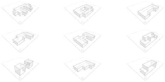
Figure 5. Single space in the building referred to as ‘Cell’.

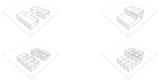
Figure 6. 18 spaces in the building, collectively known as the ‘Cell Complex’.

To achieve variation in enclosure transparency, variability was introduced to the amount and distribution of glazing across the enclosure walls and compass directions. Three levels of glazing area were considered, which are 10%, 25%, and 40% of the gross floor area. Additionally, the glazing area was distributed in five separate ways (see Table 2 and Figure 7). Furthermore, each of the 12 shapes was rotated in four directions at 90-degree intervals, resulting in the orientations north, east, south, and west. These orientations were included as variables in the simulation experiments. In total, 720 variations were generated by combining the 12 base shapes with 3 glazing area options, 5 glazing distribution patterns, and 4 orientations [6,16].

Table 2. Key Inputs and Parameters.

Category	Parameter	Value/Description
Building Features	Glazing Percentage	10%, 25%, 40%
	Orientation	North, East, South, West
	Shape Variants	12 parametric geometries (Cell, CellComplex)
	Node Attributes	Surface area, room type, aperture count, orientation
	Edge Types	Adjacency (Room-Room, Room-Aperture)
GML Parameters	GNN Layers	3 (SAGEConv layers), 3 (GINConv layers), 3 (Classic layers)
	Hidden Layer Widths	32, 32, 32–64, 64, 64–128, 128, 128
	Pooling Method	AvgPooling, MaxPooling
	Learning Rate	0.01, 0.001, 0.0001, 0.00001
	Loss Function	MSE, RMSE, MAE, MAPE, MAPE, RAE, R, R2
	Epochs	80
Random Forest	Number of Trees	90
	Criterion	MSE (regression)
	Bootstrap	Enabled
	Max Depth	Auto
Simulation Setup	Software Used	DesignBuilder + EnergyPlus
	Climate Data	Athens, Greece (TMY)
	Internal Gains	Uniform default occupancy schedule
	Wall/Window U-Values	Fixed per ASHRAE baseline

Figure 7. Three levels of glazing area were considered, which are 10%, 25%, and 40% of the gross floor area.

5.2. Energy Simulation Setting

The materials chosen for all 18 elements are consistent across all types of buildings. This selection was based on the most current and widely used materials in the construction industry, as well as their lowest U-value. The U-values for each building characteristic are as follows: walls (1.780), floors (0.860), roofs (0.500), windows (2.260).

To remain consistent with the precedent paper by [6], the simulation assumes that the buildings are situated in Athens, Greece, and are designated for residential use with a maximum of seven occupants engaged in sedentary activity (70 W). The internal design conditions were established as follows: a clothing level of 0.6 clo, humidity levels at 60%, air speed at 0.30 m/s, and lighting levels at 300 Lux. The internal heat gains were specified as 5 W/m² for sensible heat and 2 W/m² for latent heat, while the infiltration rate was set at 0.5 for the air change rate, with a wind sensitivity of 0.25 air changes per hour. Regarding thermal properties, a mixed mode with 95% efficiency was employed, with a thermostat range of 19–24 °C. The heating/cooling system was operated for 15–20 h on weekdays and 10–20 h on weekends [6,16,17]. To generate a total of 1538 data points, consisting of 769 Cells and 769 CellComplexes, the simulation was executed twice: once for generating cell datasets and once for creating CellComplexes.

In this comprehensive study, the energy simulation process was meticulously executed multiple times to cater to different datasets, each representing unique scenarios in building energy management. The initial phase of the simulation focused on the cooling dataset for a single building unit, referred to as the ‘Cell.’ This step was crucial in understanding how several factors influenced the cooling requirements of a standard building module. The simulation was then repeated for the same cell, but this time concentrating on the heating dataset. This dual approach allowed for a holistic analysis of the building’s energy needs, encompassing both heating and cooling aspects under similar conditions, thereby providing a balanced view of the energy dynamics within a single cell.

Following the detailed examination of the individual cell, the study expanded its scope to more complex structures, named ‘CellComplex’ These complexes represent a more intricate architectural arrangement, simulating a real-world scenario where spaces in a building are not isolated but part of a larger system.

6. Experimental Results

To comprehensively evaluate the predictive performance of the GML models, four key metrics were reported: Pearson’s correlation coefficient (R), coefficient of determination (R²), Mean Squared Error (MSE), and Root Mean Squared Error (RMSE). While R² is mathematically the square of R in simple linear regression, their interpretation differs in the context of non-linear and graph-based models. R provides a measure of the strength and direction of the linear relationship between predicted and actual values, while R² quantifies the proportion of variance in the dependent variable explained by the model. Including both metrics allows for a nuanced assessment of model performance. Similarly, although RMSE is the square root of MSE, both are reported to provide insight into error magnitude in squared units and interpretable units, respectively. This dual reporting facilitates comparability with other studies and supports both statistical rigor and practical understanding.

6.1. Optimizing the Hyperparameters

Initially, the entire dataset was segmented into training, validation, and testing sets. For the cooling dataset, the 767 graphs were allocated as follows: 70% for training, 10% for validation, and 20% for testing. A similar distribution was applied to the heating dataset.

As detailed below, hidden layer width, the learning rate, convolutional layer type and pooling layer, the number of epochs, and the batch size hyperparameters were varied to improve performance. The training and validation data used for tuning the hyperparameters were 630 graphs (70%).

6.1.1. Hidden Layer Width

The three experiments (No. 1, No. 2, and No. 3) compare the performance of a neural network with different hidden layer widths (see Table 3). The convolutional layer type (GINConv) and the pooling method (MaxPooling) are constant across these three experiments, and the performance is measured by the Root Mean Square Error (RMSE). The learning rate and cross-validation type are also consistent, suggesting that the variation in RMSE is due to the change in hidden layer width. Experiment No. 1: The hidden layers widths are set to 128, 128, 128. RMSE scores range from 0.9417 to 2.1524, with the best performance under the “CellComplex/heating” condition with an RMSE of 0.9417. Furthermore, experiment No. 2: The hidden layers widths are set to 64, 64, 64. RMSE scores range from 0.7524 to 2.1656, with the best performance under the “Cell/heating” condition with an RMSE of 0.7524. While experiment No. 3: The hidden layers widths are set to 32, 32, 32. RMSE scores range from 0.9291 to 2.0224, with the best performance under the “ CellComplex/heating” condition with an RMSE of 0.9291. Comparing the RMSE scores, the best-performing model in terms of the lowest RMSE is Experiment No. 2, which has hidden layers widths of 64, 64, 64. This configuration achieved the lowest RMSE of 0.7524 in the “Cell/heating” condition, suggesting that this middle ground in terms of hidden layers widths offers a better balance between model complexity and predictive performance, at least in this specific scenario. A wider hidden layer width does not automatically lead to better performance, as seen with the 128-width layers that did not perform as well as the 64-width layers. The 32-width layers also did not outperform the 64-width layers, indicating that too small a layer width might not capture enough complexity to model the data effectively. For this set of experiments and under these specific conditions, the neural network with a hidden layer width configuration of 64, 64, 64 appears to be the optimal choice among the ones assessed. Therefore, in subsequent experiments, 64-width layers were used to continue improving the accuracy of the results.

Table 3. Percentage of glazing facing on variation in direction.

	Percentage of Glazing Facing
Variation	North	East	South	West
No glazing	0	0	0	0
Uniform	25	25	25	25
North	55	15	15	15
East	15	55	15	15
South	15	15	55	15
West	15	15	15	55

6.1.2. Learning Rate

Learning rate is related to the step size at each iteration while moving toward a minimum of a loss function. The three experiments (No. 4, No. 5, and No. 6) compared the impact of different learning rates on the performance of a neural network using the GINConv convolutional layer and MaxPooling, with the performance measured by Root Mean Square Error (RMSE) (see Table 4). Experiment No. 4: Learning rate is 0.00001. RMSE ranges from 1.9254 to 2.3652, with the best performance in the “CellComplex/heating” condition at an RMSE of 1.8802. However, experiment No. 5: Learning rate is 0.001. RMSE ranges from 0.559 to 2.2171, with the best performance in the “CellComplex/heating” condition at an RMSE of 0.559. While experiment No. 6: Learning rate is 0.01. RMSE ranges from 0.5764 to 2.1638, with the best performance in the “cell/heating” condition at an RMSE of 0.5764.

Table 4. Experiments No. 1, No. 2, and No. 3.

Experiment Set No. 1		CellComplex		Cell
		Cooling	Heating	Cooling	Heating
Hyperparameters	learning rate	0.0001	0.0001	0.0001	0.0001
	cv_typ	Holdout	Holdout	Holdout	Holdout
	split	0.7, 0.1, 0.2	0.7, 0.1, 0.2	0.7, 0.1, 0.2	0.7, 0.1, 0.2
	hl_width	128, 128, 128	128, 128, 128	128, 128, 128	128, 128, 128
	conv_layer_typ	GINConv	GINConv	GINConv	GINConv
	epochs	80	80	80	80
	pooling	MaxPooling	MaxPooling	MaxPooling	MaxPooling
	batch_siz	1	1	1	1
Results	RMSE	1.2572	0.9417	2.1524	1.3871
	MAE	0.9575	0.7525	1.6902	0.7196
	MAPE	1.4306	0.7808	10.6365	4.8868
	MSE	1.5807	0.8869	4.6329	1.9241
	R	0.8616	0.108	0.6265	0.5168
	R2	0.7423	0.0117	0.3924	0.2671
	RAE	0.0144	0.0078	0.1081	0.0475
Experiment set No. 2		CellComplex		Cell
		cooling	heating	cooling	heating
Hyperparameters	learning rate	0.0001	0.0001	0.0001	0.0001
	cv_typ	Holdout	Holdout	Holdout	Holdout
	split	0.7, 0.1, 0.2	0.7, 0.1, 0.2	0.7, 0.1, 0.2	0.7, 0.1, 0.2
	hl_width	64, 64, 64	64, 64, 64	64, 64, 64	64, 64, 64
	conv_layer_typ	GINConv	GINConv	GINConv	GINConv
	epochs	80	80	80	80
	pooling	MaxPooling	MaxPooling	MaxPooling	MaxPooling
	batch_siz	1	1	1	1
Results	RMSE	1.4246	1.433	2.1656	0.7524
	MAE	1.058	0.6728	1.5917	0.5319
	MAPE	1.5796	0.6969	9.6537	3.5263
	MSE	2.0294	2.0535	4.6897	0.5661
	R	0.8025	0.0797	0.6058	0.8058
	R2	0.6441	0.0063	0.367	0.6493
	RAE	0.0159	0.007	0.1008	0.0351
Experiment set No. 3		CellComplex		Cell
		cooling	heating	cooling	heating
Hyperparameters	learning rate	0.0001	0.0001	0.0001	0.0001
	cv_typ	Holdout	Holdout	Holdout	Holdout
	split	0.7, 0.1, 0.2	0.7, 0.1, 0.2	0.7, 0.1, 0.2	0.7, 0.1, 0.2
	hl_width	32, 32, 32	32, 32, 32	32, 32, 32	32, 32, 32
	conv_layer_typ	GINConv	GINConv	GINConv	GINConv
	epochs	80	80	80	80
	pooling	MaxPooling	MaxPooling	MaxPooling	MaxPooling
	batch_siz	1	1	1	1
Results	RMSE	1.6912	0.9291	2.0224	0.9552
	MAE	1.1998	0.5768	1.5927	0.6949
	MAPE	1.7882	0.5964	10.2843	4.5139
	MSE	2.8603	0.8633	4.09	0.9124
	R	0.7474	−0.0392	0.6034	0.6984
	R2	0.5586	0.0015	0.3641	0.4878
	RAE	0.0181	0.006	0.1049	0.0453

Based on the RMSE values, the best learning rate among those assessed is 0.001 (Experiment No. 5), as it resulted in the lowest RMSE of 0.559 under the “CellComplex/cooling” condition. A lower RMSE indicates a model that is better at predicting the target variable with fewer errors, and thus it can be inferred that the learning rate of 0.001 is the most effective for this neural network configuration and dataset. Therefore, in subsequent experiments, we used this learning rate to continue improving the accuracy of the results.

6.1.3. Pooling Layer

The two experiments (No. 2 and No. 9) compared the performance of a neural network with different pooling layers: MaxPooling in Experiment No. 2 and AvgPooling in Experiment No. 9 (see Table 5). Other hyperparameters, such as learning rate, cross-validation type, split, hidden layer width, and convolutional layer type, are held constant across both experiments. The performance of the network is evaluated using Root Mean Square Error (RMSE). Experiment No. 2 (MaxPooling): The RMSE values range from 0.7524 to 2.1656. The best performance in this experiment is observed under the “cell/heating” condition with an RMSE of 0.7524. Moreover, experiment No. 9 (AvgPooling): The RMSE values range from 0.2205 to 2.0393. The best performance in this experiment is observed under the “CellComplex/heating” condition with an RMSE of 0.2205. Based on the RMSE values, AvgPooling in Experiment No. 9 shows the best performance with the lowest RMSE of 0.2205 under the “CellComplex/heating” condition, suggesting that AvgPooling layer may be more effective for this particular network architecture and dataset. Therefore, in subsequent experiments, we used AvgPooling to continue improving the accuracy of the results.

Table 5. Experiments No. 4, No. 5, and No. 6.

Experiment Set No. 4		CellComplex		Cell
		Cooling	Heating	Cooling	Heating
Hyperparameters	learning rate	0.00001	0.00001	0.00001	0.00001
	cv_typ	Holdout	Holdout	Holdout	Holdout
	split	0.7, 0.1, 0.2	0.7, 0.1, 0.2	0.7, 0.1, 0.2	0.7, 0.1, 0.2
	hl_width	64, 64, 64	64, 64, 64	64, 64, 64	64, 64, 64
	conv_layer_typ	GINConv	GINConv	GINConv	GINConv
	epochs	80	80	80	80
	pooling	MaxPooling	MaxPooling	MaxPooling	MaxPooling
	batch_siz	1	1	1	1
Results	RMSE	1.9254	2.3213	2.3652	1.8802
	MAE	1.3774	1.2154	1.8194	1.3382
	MAPE	2.0865	1.2587	11.473	9.0812
	MSE	3.7071	5.3882	5.594	3.5352
	R	0.6371	−0.0655	0.6362	0.6272
	R2	0.4059	0.004	0.4048	0.3934
	RAE	0.0208	0.0126	0.1158	0.0881
Experiment set No. 5		CellComplex		Cell
		cooling	heating	cooling	heating
Hyperparameters	learning rate	0.001	0.001	0.001	0.001
	cv_typ	Holdout	Holdout	Holdout	Holdout
	split	0.7, 0.1, 0.2	0.7, 0.1, 0.2	0.7, 0.1, 0.2	0.7, 0.1, 0.2
	hl_width	64, 64, 64	64, 64, 64	64, 64, 64	64, 64, 64
	conv_layer_typ	GINConv	GINConv	GINConv	GINConv
	epochs	80	80	80	80
	pooling	MaxPooling	MaxPooling	MaxPooling	MaxPooling
	batch_siz	1	1	1	1
Results	RMSE	1.7719	0.559	2.2171	0.6857
	MAE	1.5088	0.4506	1.5817	0.4505
	MAPE	2.2898	0.4667	9.6008	2.9997
	MSE	3.1397	0.3125	4.9157	0.4701
	R	0.8631	0.2968	0.5787	0.8232
	R2	0.745	0.0881	0.3349	0.6777
	RAE	0.0228	0.0047	0.1007	0.0297
Experiment set No. 6		CellComplex		Cell
		cooling	heating	cooling	heating
Hyperparameters	learning rate	0.01	0.01	0.01	0.01
	cv_typ	Holdout	Holdout	Holdout	Holdout
	split	0.7, 0.1, 0.2	0.7, 0.1, 0.2	0.7, 0.1, 0.2	0.7, 0.1, 0.2
	hl_width	64, 64, 64	64, 64, 64	64, 64, 64	64, 64, 64
	conv_layer_typ	GINConv	GINConv	GINConv	GINConv
	epochs	80	80	80	80
	pooling	MaxPooling	MaxPooling	MaxPooling	MaxPooling
	batch_siz	1	1	1	1
Results	RMSE	2.1638	1.7054	1.8569	0.5764
	MAE	1.889	1.5617	1.3772	0.4178
	MAPE	2.8708	1.6199	8.3608	2.7437
	MSE	4.6822	2.9082	3.448	0.3322
	R	0.8536	0.0631	0.6706	0.8779
	R2	0.7286	0.004	0.4497	0.7707
	RAE	0.0286	0.0162	0.0876	0.0275

6.1.4. Convolutional Layer Type

The type of convolutional layer varies across experiments with GINConv used in No. 7, SAGEConv in No. 8, and Classic in No. 9 (see Table 6). Experiment No. 7 uses “GINConv” convolutional layers. The RMSE scores range from 0.3702 to 2.1839, with the lowest RMSE observed under the “CellComplex/heating” condition at 0.3702. Moreover, experiment No. 8 uses “SAGEConv” convolutional layers. The RMSE scores here range from 0.2158 to 2.0855, with the lowest RMSE again observed under the “CellComplex/heating” condition at 0.2158. Furthermore, experiment No. 9 uses “Classic” convolutional. The RMSE scores range from 0.2205 to 2.0393, with the lowest RMSE observed under the “CellComplex/heating” condition at 0.2205. Based on the RMSE values presented, “SAGEConv” convolutional layers in Experiment No. 8 demonstrate the best performance with the lowest RMSE of 0.2158, indicating it as the most accurate model under the “CellComplex/heating” condition among the three experiments. Therefore, in subsequent experiments, we used SAGEConv layer type to continue improving the accuracy of the results.

Table 6. Experiments No. 9.

Experiment Set No. 9		CellComplex		Cell
		Cooling	Heating	Cooling	Heating
Hyperparameters	learning rate	0.001	0.001	0.001	0.001
	cv_typ	Holdout	Holdout	Holdout	Holdout
	split	0.7, 0.1, 0.2	0.7, 0.1, 0.2	0.7, 0.1, 0.2	0.7, 0.1, 0.2
	hl_width	64, 64, 64	64, 64, 64	64, 64, 64	64, 64, 64
	conv_layer_typ	Classic	Classic	Classic	Classic
	epochs	80	80	80	80
	pooling	AvgPooling	AvgPooling	AvgPooling	AvgPooling
	batch_siz	1	1	1	1
Results	RMSE	0.8247	0.2205	2.0393	0.784
	MAE	0.6756	0.1806	1.4127	0.6108
	MAPE	1.0208	0.1868	8.3763	4.0768
	MSE	0.6801	0.0486	4.1588	0.6147
	R	0.9585	0.9367	0.659	0.8291
	R2	0.9187	0.8774	0.4343	0.6874
	RAE	0.0102	0.0019	0.09	0.0401

6.1.5. Cross Validation Type

The two experiments (No. 8 and No. 9) compared the performance of a neural network with the SAGEConv convolutional layer type using different cross-validation (CV) strategies: “Holdout” in Experiment No. 8 and “10 k_folds” in Experiment No. 9. The performance of the neural network is measured using the Root Mean Square Error (RMSE), with both experiments maintaining a constant learning rate of 0.001. Experiment No. 8 (Holdout CV): The RMSE values range from 0.2158 to 2.0855. The best performance is observed under the “CellComplex/heating” condition with an RMSE of 0.2158. Moreover, experiment No. 9 (10 k_folds CV): The RMSE values range from 0.1739 to 1.9675. The best performance is observed under the “CellComplex/heating” condition with an RMSE of 0.1739. Based on the provided RMSE values, the “10 k_folds” cross-validation technique used in Experiment No. 9 seems to be the better method for evaluating the neural network’s performance, as it achieved the lowest RMSE of 0.1739 in the “CellComplex/heating” condition. This suggests that using a k-fold cross-validation provides a more reliable estimate of the model’s generalization to new data compared to the holdout method. However, the drawback of using k-fold cross-validation is that it requires a more powerful computer and additional time.

6.1.6. Sensitivity to Hyperparameter Changes

The tuning results indicate that model performance is most sensitive to changes in the convolutional layer type and learning rate. Switching from GINConv to SAGEConv led to an RMSE reduction of up to 41%, especially in heating prediction tasks. Similarly, increasing the learning rate from 0.00001 to 0.001 significantly improved convergence and lowered RMSE values. Conversely, changes in hidden layer width had a moderate effect, with diminishing returns beyond 64 units. The choice of pooling method (AvgPooling vs. MaxPooling) also contributed to performance variation, especially in smaller datasets. These findings suggest that proper selection of convolution layers and learning rate is critical for achieving optimal GML performance in building energy prediction tasks.

6.2. Testing the Machine Learning DGL

After tuning the hyperparameters, the best performing model was saved and tested on the test set. As mentioned above, the data was split as 70% for training, 10% for validation, and 20% for testing. In this stage we used a 20% portion of the data to run the testing. The DGL parameters were as follows: learning rate of 0.001, hidden layer width 64,64,64, with AvgPooling layer, 80 epochs SAGEConv for the convolutional layer type, Holdout cross validation type, and batch size of 1. The result of the final test was: For “CellComplex” under “cooling,” RMSE is 0.8805. For “CellComplex” under “heating,” RMSE is 0.2158. For “Cell” under “cooling,” RMSE is 2.0855. For “Cell” under “heating,” RMSE is 0.8238.

A comparison of actual values and predicted values was described in (Table 7). Each row represents a single observation or test case, with the first number being the actual value observed or measured, and the second number being the value that the model predicted for that same case.

Table 7. Experiments (No. 7, and No. 8).

Experiment Set No. 7		CellComplex		Cell
		Cooling	Heating	Cooling	Heating
Hyperparameters	learning rate	0.001	0.001	0.001	0.001
	cv_typ	Holdout	Holdout	Holdout	Holdout
	split	0.7, 0.1, 0.2	0.7, 0.1, 0.2	0.7, 0.1, 0.2	0.7, 0.1, 0.2
	hl_width	64, 64, 64	64, 64, 64	64, 64, 64	64, 64, 64
	conv_layer_typ	GINConv	GINConv	GINConv	GINConv
	epochs	80	80	80	80
	pooling	AvgPooling	AvgPooling	AvgPooling	AvgPooling
	batch_siz	1	1	1	1
Results	RMSE	0.9526	0.3702	2.1839	0.6255
	MAE	0.7201	0.3158	1.5367	0.4277
	MAPE	1.0887	0.327	9.3178	2.8303
	MSE	0.9075	0.1371	4.7696	0.3912
	R	0.9297	0.9182	0.6845	0.8417
	R2	0.8643	0.843	0.4686	0.7085
	RAE	0.0109	0.0033	0.1001	0.0283
Experiment set No. 8		CellComplex		Cell
		cooling	heating	cooling	heating
Hyperparameters	learning rate	0.001	0.001	0.001	0.001
	cv_typ	Holdout	Holdout	Holdout	Holdout
	split	0.7, 0.1, 0.2	0.7, 0.1, 0.2	0.7, 0.1, 0.2	0.7, 0.1, 0.2
	hl_width	64, 64, 64	64, 64, 64	64, 64, 64	64, 64, 64
	conv_layer_typ	SAGEConv	SAGEConv	SAGEConv	SAGEConv
	epochs	80	80	80	80
	pooling	AvgPooling	AvgPooling	AvgPooling	AvgPooling
	batch_siz	1	1	1	1
Results	RMSE	0.8805	0.2158	2.0855	0.8238
	MAE	0.72	0.1762	1.5363	0.6276
	MAPE	1.0913	0.1825	9.561	4.14
	MSE	0.7754	0.0465	4.3492	0.6786
	R	0.9367	0.9455	0.6595	0.6893
	R2	0.8773	0.894	0.435	0.4751
	RAE	0.0109	0.0018	0.0983	0.0412

To analyze this:

• Closeness of Values: The predicted values are quite close to the actual values, which suggests that the predictive model is performing relatively well.
• Consistency: The model exhibits a consistent underestimation of actual values despite strong correlation, likely due to the asymmetric distribution of the target variable and the use of a symmetric loss function (e.g., MSE), which biases predictions toward the center of the distribution. Future work will explore target transformations and alternative loss functions, such as quantile or asymmetric losses, to improve prediction accuracy across the full value range.
• Error Measurement: To quantify the model performance, an error is calculated for each prediction. Common methods include the absolute error (the absolute difference between actual and predicted).

In the example above, the absolute error is calculated by subtracting the predicted value from the actual value and taking the absolute value of the result. This is performed for each pair of actual and predicted values.

For a more detailed analysis and observation, a Scatter Plot was generated (see Figure 8). Most data points in the plot are relatively close to the perfect prediction line, suggesting that the model generally achieves a satisfactory level of accuracy. This indicates that, in most cases, the predicted values are reasonably close to the actual values.

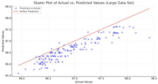
Figure 8. Scatter plot of the relationship between actual and predicted energy load values for the large dataset. The red dashed line represents the ideal case where predicted values match actual values.

However, some data points are scattered away from the perfect prediction line, highlighting specific instances where the model’s predictions are less accurate. These instances suggest that, while the model performs well overall, there are certain cases or patterns that it may not be capturing effectively.

The line graph (see Figure 9) comparing actual values to predicted values over a series of data points. The two lines in the graph, one representing the actual values and the other representing the predicted values, to visualize the performance of a predictive model. Both values show similar patterns, indicating that the predicted values are following the actual values closely. This is indicative of a model that has learned the underlying pattern in the data well.

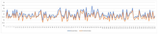
Figure 9. Comparison of actual versus predicted heating and cooling loads. The line graph shows predicted values tracking actual simulation results over test data points. Axis labels indicate energy load in kWh. Close alignment indicates model accuracy.

6.3. Random Forest Baseline

This section presents the experiment using RF algorithms, which serve as a baseline model. Random Forest, an advancement of Decision Trees (DT), is employed in regression learning for modeling heating and cooling loads. The input features for RF modeling mirror those discussed in Section 5, having undergone pre-processing in preparation for (DGL) modeling. The output of the model is focused on predicting heating and cooling loads.

Numerous hyperparameters play a crucial role in achieving an accurate RF model. This experiment specifically addresses parameters such as (1) the number of trees, (2) bootstrap, and (3) the minimal cost-complexity pruning parameter (ccp_alphas). To fine-tune these hyperparameters, a systematic search is conducted with a k-fold cross-validation experiment. In k-fold cross-validation, the data are divided into k folds, with (k − 1) folds allocated to training and the remaining one to testing. The experiments are iterated k times, ensuring that each fold is part of both training and testing sets across different iterations.

After the hyperparameter tuning, the optimal results of each experiment, as presented in (see Table 8 and Table 9), are summarized as follows:

Table 8. An example of how one might calculate the absolute errors for given data.

Actual Value	Predicted Value	Absolute Error
96.636	96.3291	0.3069
97.761	97.3508	0.4102
96.267	96.3119	0.0449
96.984	96.635	0.349
96.50	96.3282	0.1718
96.626	96.4564	0.1696
96.685	96.6478	0.0372
97.59	97.1392	0.4508
96.752	96.3426	0.4094
97.835	97.1421	0.6929
96.407	96.326	0.081

Table 9. Random Forest optimal results.

Final Optimized Results		CellComplex		Cell
		Cooling	Heating	Cooling	Heating
Hyperparameters	learning rate	0.001	0.001	0.001	0.001
	cv_typ	K-Fold	K-Fold	K-Fold	K-Fold
	n_splits	5 folds	5 folds	5 folds	5 folds
	Data Split	80, 20	80, 20	80, 20	80, 20
	number of trees	80	90	70	90
	bootstrap_opt	Enabled	Enabled	Enabled	Enabled
	ccp_alphas	0	0	0	0
Results	RMSE	0.04964	0.03126	0.05650	0.03644
	MAE	0.16994	0.14156	0.17528	0.14931
	R2	0.98894	0.99493	0.99085	0.99423

CellComplex (cooling loads): The results are for the bootstrap option enabled, with a total of 80 trees. The final test results were as follows: the RMSE was 0.04964, the MAE was 0.16994, and the R² score was 0.98894.

CellComplex (heating loads): From the experiment, the optimal model had the following hyperparameter combination: Bootstrap option enabled and a total of 90 trees. The final test results were as follows: the RMSE was 0.03126, the MAE was 0.14156, and the R² score was close to one.

Cell (cooling loads): The results are for the bootstrap option enabled, with a total of 70 trees. The final test results were as follows: the RMSE was 0.05650, the MAE was 0.17528, and the R² score was 0.99085.

Cell (heating loads): From the experiment, the optimal model had the following hyperparameter combination: Bootstrap option enabled and a total of 90 trees. The final test results were as follows: the RMSE was 0.03644, the MAE was 0.14931, and the R² score was 0.99423.

The results demonstrated that RF algorithms exhibit high accuracy in predicting heating and cooling loads. Furthermore, an increase in the number of trees generally aligns with improved performance. Although the influence on performance due to enabling or disabling the bootstrap option is not conspicuous, its absence leads to a reduction in overall performance.

6.4. Physical Explanations of Trends and Practical Applications

The trends observed in the results can be explained by the underlying physical principles governing building thermal performance. For example, lower RMSE values in the heating load predictions for the CellComplex models reflect the advantage of explicitly modeling spatial connectivity and adjacency between zones, which is critical in heat transfer analysis. The higher accuracy in heating prediction compared to cooling may also be attributed to more consistent internal gains and the envelope’s thermal resistance in heating-dominated conditions.

The Random Forest baseline performed exceptionally well (R² > 0.99) because of its ability to capture non-linear relationships in the synthetic dataset, which includes structured variations in glazing ratios (10%, 25%, 40%), orientations (north, east, south, west), and surface areas. However, Random Forest models flatten this information and cannot directly capture topological relationships. Graph machine learning (GML), in contrast, leverages node and edge connectivity to maintain adjacency relationships critical for realistic energy modeling, explaining its robust performance even when tested with cross-validation.

From a practical perspective, these results highlight how GML can support early design decision-making in architecture and engineering. By integrating topological data directly into the prediction model, GML enables more realistic energy consumption estimates for novel design configurations without requiring detailed, time-consuming simulations for every variant. This capability is essential for rapid evaluation of design alternatives, supporting goals of energy-efficient design, code compliance, and smart building integration with IoT systems for real-time energy optimization.

6.5. Comparative Analysis and Discussion of Alternative Approaches

To contextualize the benefits of graph machine learning (GML) in this study, it is important to consider how it compares to other machine learning approaches, including Convolutional Neural Networks (CNNs) and hybrid models. While CNNs excel in domains with regular grid structures such as image data, their architecture is inherently limited when applied to irregular, non-Euclidean data like building topology graphs. In building energy modeling, the relationships between rooms, walls, floors, and apertures form complex, non-grid-like graphs where connectivity and adjacency vary per design. GML models, by design, can naturally incorporate these topological features through node and edge representations, enabling them to capture thermal interactions in ways that CNNs cannot.

In this study, we included Random Forest (RF) as a strong baseline method. RF models are effective in capturing non-linear relationships and achieved very high accuracy (e.g., RMSE as low as 0.03126 for heating loads in CellComplex configurations with R² > 0.99). However, RF relies on flattened, tabular representations of features and does not inherently model spatial connectivity. In contrast, GML achieves comparable accuracy (best RMSE of 0.1739 with 10-fold cross-validation) while explicitly preserving building topology. This ability to directly encode graph structure offers significant benefits for generalizing to diverse architectural designs.

Hybrid models that combine GML with other neural network components (e.g., sequence models for temporal occupancy patterns, CNN modules for façade image analysis) represent a promising avenue for future research. While this study focused on establishing a graph-based framework for static topological and geometric features, integrating hybrid methods could enable richer multi-modal analysis, combining topology with sensor data, temporal schedules, or image-based façade features.

By highlighting these differences, this comparison underscores the unique suitability of GML for the challenge of estimating building heating and cooling loads while identifying opportunities for expanding the framework with complementary techniques.

6.6. Feature Importance and Topological Contribution

Understanding how different topological features contribute to model predictions is critical for interpreting graph machine learning (GML) outputs in the context of building energy analysis. In this study, each node is labeled by type (e.g., wall, floor, aperture), and topological features such as surface area, orientation, and adjacency counts are embedded as node attributes. Edges represent spatial relationships, primarily room-to-room and room-to-aperture connections. While traditional ML models such as Random Forests offer explicit feature importance scores, explainability in GML is more complex. To assess the influence of topological features, we adopted several strategies. First, experiments revealed that denser graphs—those with higher node degree centrality—tended to result in better performance, especially in heating load predictions. This suggests that thermal adjacency relationships (captured via edges) enhance the model’s ability to learn heat transfer across connected spaces. Second, while edges in this study were treated as unweighted, future extensions will consider encoding edge weights based on thermal resistance or adjacency area to better reflect physical interactions and their impact on energy transfer.

7. Conclusions

This paper presented a novel approach in graph machine learning, aimed at improving the estimation of heating and cooling loads in buildings, a crucial aspect of building energy efficiency. Traditional methods in this domain often fall short in capturing the complex relationship between a building’s topological, geometric, and physical characteristics, leading to predictions that lack precision. This research successfully addresses this gap by integrating these critical factors into a graph-based machine learning framework.

A significant contribution of this work is the development of a parametric generative workflow, building upon the methodology of [6]. This workflow enabled the creation of a synthetic dataset, which is a cornerstone of this study. This dataset is comprehensive, encompassing various building forms with distinct topological connections and attributes. It facilitated extensive analysis across different building scenarios, enhancing the robustness and applicability of this finding.

This research involved simulating a wide range of building shapes and glazing scenarios, incorporating variations in window sizes and orientations. The results from thermal simulations provided a rich dataset for this machine learning analysis. We employed Deep Graph Learning (DGL) as a primary method for training and used decision trees (DT) for validation purposes. Both the DGL and DT algorithms showed high efficacy in predicting heating and cooling loads, thereby making a significant contribution to the field of building energy efficiency.

In this study, a series of experiments were conducted to optimize the hyperparameters of a graph-based machine learning model for predicting heating and cooling loads in buildings. The experiments involved adjusting variables such as a hidden layer width, a learning rate, a pooling layer, a convolutional layer type, and a cross-validation type. Notable findings include the identification of an optimal hidden layer’s widths of 64, 64, 64, a learning rate of 0.001, the effectiveness of the AvgPooling layer, and the superiority of the SAGEConv convolutional layer. The “10 k_folds” cross-validation method outperformed the holdout method, providing more reliable estimates. The final model, tested on a separate dataset, demonstrated high accuracy, with predicted values closely matching the actual values, as evidenced by low Root Mean Square Error (RMSE) scores and a comparison of actual versus predicted values in the test cases. This highlights the model’s effectiveness in accurately predicting building energy needs, which illustrates the potential of machine learning in enhancing energy efficiency in the architectural domain.

In conclusion, this study highlights the transformative potential of machine learning in optimizing building designs for energy efficiency. By delivering more accurate predictions of heating and cooling loads, this approach advances research at the intersection of machine learning, architecture, and sustainability. This work establishes a framework for smarter, energy-efficient buildings, supporting broader goals in environmental sustainability and energy conservation.

8. Limitations and Future Work

Despite the promising results achieved through graph machine learning (GML) in predicting building heating and cooling loads, several limitations and challenges remain. A primary concern is the reliance on a synthetically generated dataset created through a parametric workflow. While this ensures systematic control and reproducibility, it may not fully capture the complex variability and nuanced characteristics of real-world buildings, thereby limiting the model’s direct applicability without further empirical validation.

Another challenge lies in the scalability and generalizability of the proposed method. As the size and complexity of the dataset increase, so do the computational requirements—particularly when using deep graph neural networks, k-fold cross-validation, and multiple convolutional architectures. These demands may hinder large-scale deployment or application in resource-constrained environments.

Geographic and climatic assumptions present further limitations. The simulations are based solely on conditions in Athens, Greece, restricting generalizability to regions with different climatic profiles. Additionally, fixed internal loads, occupant behavior, and HVAC schedules in the simulations fail to reflect the dynamic and unpredictable nature of real-world building operations.

The current model is also purely data-driven and does not incorporate physical laws. This limits its interpretability and robustness under changing boundary conditions. Future work could integrate physics-informed learning—such as embedding heat conduction equations—through techniques like physics-informed neural networks (PINNs) or physics-constrained GNNs. This hybrid modeling approach may enhance both predictive accuracy and physical interpretability.

To overcome current limitations, future research will incorporate empirical datasets from Building Information Models (BIM), laser scanning, and IoT-enabled sensor networks to validate GML models against actual building performance. Accurate 3D digital models capturing spatial relationships such as adjacency and connectivity will be essential. Where such models are unavailable, 3D scanning technologies can be employed, with the data processed via TopologicPy to generate graph representations suitable for GML analysis.

Furthermore, exploring optimization techniques—including hyperparameter tuning, graph pruning, and integrating alternative learning methods such as reinforcement learning or transfer learning—will help improve adaptability and scalability. This methodology could also extend to urban-scale analysis, influencing city-wide energy strategies and sustainable development. Finally, these insights can enrich architectural and engineering education by emphasizing AI and ML’s growing role in sustainable design.

To further support practical design and retrofitting decisions, future work will integrate explainable AI (XAI) techniques into the modeling pipeline. While graph machine learning models are inherently less interpretable, emerging XAI methods such as GNNExplainer, Integrated Gradients, and Saliency Maps offer tools to identify the most influential nodes, features, and edge structures contributing to heating and cooling load predictions. By quantifying the importance of input features—such as surface area, aperture count, orientation, and topological adjacency—XAI can offer architects and engineers transparent insights into how specific design attributes affect energy outcomes. This capability can inform envelope optimization strategies that comply with code requirements while enhancing building performance.

Finaly graph machine learning (GML), especially with 10-fold cross-validation, requires substantial computational resources. For this study, each k-fold training cycle for the DGL model (including AvgPooling, SAGEConv layers, and 80 epochs) required approximately 12–15 min on a mid-range GPU (NVIDIA RTX 3060, 12 GB VRAM), amounting to ~1.2–1.5 h for full 10-fold validation. Random Forest (with 90 trees and bootstrap enabled) was considerably faster, with k-fold runs taking 15–20 min on a standard CPU (Intel i7, 16 GB RAM). These resource demands underscore the need to balance model complexity with practical training time, particularly for large-scale deployment or real-time applications in smart building systems.

References

- Zhong, H.; Wang, J.; Jia, H.; Mu, Y.; Lv, S. Vector Field-Based Support Vector Regression for Building Energy Consumption Prediction. Appl. Energy 2019, 242, 403–414. [Google Scholar] [CrossRef]
- Dong, B.; Cao, C.; Lee, S.E. Applying Support Vector Machines to Predict Building Energy Consumption in Tropical Region. Energy Build. 2005, 37, 545–553. [Google Scholar] [CrossRef]
- Wei, Y.; Xia, L.; Pan, S.; Wu, J.; Zhang, X.; Han, M.; Zhang, W.; Xie, J.; Li, Q. Prediction of Occupancy Level and Energy Consumption in Office Building Using Blind System Identification and Neural Networks. Appl. Energy 2019, 240, 276–294. [Google Scholar] [CrossRef]
- Ekici, B.B.; Aksoy, U.T. Prediction of Building Energy Consumption by Using Artificial Neural Networks. Adv. Eng. Softw. 2009, 40, 356–362. [Google Scholar] [CrossRef]
- Rahman, A.; Srikumar, V.; Smith, A.D. Predicting Electricity Consumption for Commercial and Residential Buildings Using Deep Recurrent Neural Networks. Appl. Energy 2018, 212, 372–385. [Google Scholar] [CrossRef]
- Chou, J.S.; Dac, K.B. Modeling Heating and Cooling Loads by Artificial Intelligence for Energy-Efficient Building Design. Energy Build. 2014, 82, 437–446. [Google Scholar] [CrossRef]
- Pan, Y.; Zhu, M.; Lv, Y.; Yang, Y.; Liang, Y.; Yin, R.; Yang, Y.; Jia, X.; Wang, X.; Zeng, F.; et al. Building Energy Simulation and Its Application for Building Performance Optimization: A Review of Methods, Tools, and Case Studies. Adv. Appl. Energy 2023, 10, 100135. [Google Scholar] [CrossRef]
- Gonzalo, A.D.F.; Santamaría, B.M.; Burgos, M.J.M. Assessment of Building Energy Simulation Tools to Predict Heating and Cooling Energy Consumption at Early Design Stages. Sustainability 2023, 15, 1920. [Google Scholar] [CrossRef]
- Harish, V.S.K.V.; Kumar, A. A Review on Modeling and Simulation of Building Energy Systems. Renew. Sustain. Energy Rev. 2016, 56, 1272–1292. [Google Scholar] [CrossRef]
- Subramanian, A.S.R.; Gundersen, T.; Adams, T.A. Modeling and Simulation of Energy Systems: A Review. Processes 2018, 6, 238. [Google Scholar] [CrossRef]
- Aish, R.; Jabi, W.; Lannon, S.; Wardhana, N.; Chatzivasileiadi, A. Topologic: Tools to Explore Architectural Topology. In Proceedings of the AAG 2018: Advances in Architectural Geometry 2018, Gothenburg, Sweden, 22–25 September 2018; pp. 316–341. [Google Scholar]
- Jabi, W.; Aish, R.; Lannon, S.; Chatzivasileiadi, A.; Wardhana, N.M. Topologic a Toolkit for Spatial and Topological Modelling. In Shape, Form & Geometry; Springer: Berlin/Heidelberg, Germany, 2018; Available online: http://papers.cumincad.org/data/works/att/ecaade2018_310.pdf (accessed on 28 August 2025).
- Jabi, W. Linking Design and Simulation Using Non-Manifold Topology. Archit. Sci. Rev. 2016, 59, 323–334. [Google Scholar] [CrossRef]
- Jabi, W. The Potential of Non-Manifold Topology in the Early Design Stages. In Proceedings of the ACADIA 2015—Computational Ecologies: Design in the Anthropocene: Proceedings of the 35th Annual Conference of the Association for Computer Aided Design in Architecture, Cincinnati, OH, USA, 19–25 October 2015. [Google Scholar]
- Chatzivasileiadi, A.; Simon, L.; Wassim, J.; Nicholas, M.W.; Robert, A. Addressing Pathways to Energy Modelling through Non-Manifold Topology. Simul. Ser. 2018, 50, 31–38. [Google Scholar] [CrossRef]
- Pessenlehner, W.; Mahdavi, A. Building Morphology, Transparence and Energy Performance. In Proceedings of the Building Simulation 2003, Eindhoven, The Netherlands, 11–14 August 2003; pp. 1025–1032. [Google Scholar]
- Tsanas, A.; Xifara, A. Accurate Quantitative Estimation of Energy Performance of Residential Buildings Using Statistical Machine Learning Tools. Energy Build. 2012, 49, 560–567. [Google Scholar] [CrossRef]
- Moayedi, H.; Bui, D.T.; Dounis, A.; Lyu, Z.; Foong, L.K. Predicting Heating Load in Energy-Efficient Buildings through Machine Learning Techniques. Appl. Sci. 2019, 9, 4338. [Google Scholar] [CrossRef]
- Yan, Z.; Zhu, X.; Wang, X.; Ye, Z.; Guo, F.; Xie, L.; Zhang, G. A multi-energy load prediction of a building using the multi-layer perceptron neural network method with different optimization algorithms. Energy Explor. Exploit. 2023, 41, 273–305. [Google Scholar] [CrossRef]
- Ahmad, M.W.; Jonathan, R.; Yacine, R. Random Forests and Artificial Neural Network for Predicting Daylight Illuminance and Energy Consumption. Build. Simul. 2017, 15, 1949–1955. [Google Scholar]
- Tung, K.Y.; Huang, I.C.; Chen, S.L.; Shih, C.T. Mining the Generation Xers’ Job Attitudes by Artificial Neural Network and Decision Tree—Empirical Evidence in Taiwan. Expert Syst. Appl. 2005, 29, 783–794. [Google Scholar] [CrossRef]
- Tso, G.K.F.; Yau, K.K.W. Predicting Electricity Energy Consumption: A Comparison of Regression Analysis, Decision Tree and Neural Networks. Energy 2007, 32, 1761–1768. [Google Scholar] [CrossRef]
- Yu, Z.; Haghighat, F.; Fung, B.C.M.; Yoshino, H. A Decision Tree Method for Building Energy Demand Modeling. Energy Build. 2010, 42, 1637–1646. [Google Scholar] [CrossRef]
- Alammar, A.; Jabi, W.; Lannon, S. Predicting Incident Solar Radiation on Building’s Envelope Using Machine Learning; SimAUD: Madrid, Spain, 2021. [Google Scholar]
- Alammar, A.; Jabi, W. Generation of a Large Synthetic Database of Office Tower’s Energy Demand Using Simulation and Machine Learning. In Formal Methods in Architecture; Mora, P.L., Viana, D.L., Morais, F., Vaz, J.V., Eds.; Springer Nature: Singapore, 2023; pp. 479–500. [Google Scholar]
- Jabi, W.; Alymani, A. Graph Machine Learning Using 3D Topological Models; SimAUD: Madrid, Spain, 2020; pp. 427–434. [Google Scholar]
- Alymani, A.; Jabi, W.; Corcoran, P. Graph Machine Learning Classification Using Architectural 3D Topological Models. Simul. Trans. Soc. Model. Simul. Int. 2022, 99, 1117–1131. [Google Scholar] [CrossRef]
- Alymani, A.; Jabi, W. Modelling the Relationships between Ground and Buildings Using Architectural Topological Models Utilizing Graph Machine Learning. In Proceedings of the 6th International Symposium Formal Methods in Architecture, A Coruña, Spain, 24–27 May 2022. [Google Scholar]
Disclaimer/Publisher’s Note: The statements, opinions and data contained in all publications are solely those of the individual author(s) and contributor(s) and not of MDPI and/or the editor(s). MDPI and/or the editor(s) disclaim responsibility for any injury to people or property resulting from any ideas, methods, instructions or products referred to in the content. |
© 2025 by the authors. Licensee MDPI, Basel, Switzerland. This article is an open access article distributed under the terms and conditions of the Creative Commons Attribution (CC BY) license (https://creativecommons.org/licenses/by/4.0/).