Multiperiod Location–Allocation Optimization of Construction Logistics Centers for Large-Scale Projects in Complex Environmental Regions

Abstract

As an efficient management pattern to improve logistics efficiency through intensive management of construction materials, construction logistics centers (CLCs) have received active attention from academics and practitioners. However, the CLC location–allocation problem, which considers periodic demand and transportation risk, has not been adequately solved. This work provides an approach to integrating transportation path risk into multiperiod CLC location–allocation optimization for large-scale projects in complex environmental regions. For this purpose, this paper formulates a hybrid non-linear integer planning model to define this location–allocation problem and minimize the total cost of construction logistics and transportation risk. The model also incorporates critical features from realistic scenarios, including CLC’s service coverage, capacity constraints, and minimum utilization limits. We have designed an NSGA-II based on endocrine hormone regulation (EHR-NSGA-II) to solve the model. Finally, a large-scale railroad construction project in complex environmental regions is used as an example to prove the effectiveness of the model and algorithm. Compared with the single-period model, the multiperiod model designed in this paper provides a total cost reduction of 8.11% for the CLC location–allocation scheme. In addition, analyzing several key parameters provides valuable insights for managers to design more reliable construction logistics networks.

1. Introduction

Construction accounts for approximately 13% of the world’s gross domestic product and is an industry of great economic significance and global influence [1]. The main activity of a construction project is to receive construction materials from different suppliers from all over the country or even the world and assemble them into a complex and unique final product through a complicated process [2,3]. On-time and on-quantity delivery of construction materials to construction sites is a prerequisite for adequately executing a construction project [4]. Delays in the delivery of construction materials may disrupt the construction program, affecting the project’s schedule, cost, and quality [5]. According to statistics, an average Swedish construction worker spends over 50% of his time waiting for and handling construction materials [6]. Non-value-added costs due to the improper delivery of construction materials accounted for 7–12% of the total expenses on a construction project in China [7]. To promote the sustainable development of the construction industry, many scholars have studied ways to improve the organization model of construction activities to increase the efficiency of construction logistics [7,8]. Among these, construction logistics management is recognized by both academia and industry as a potential frontier for improving the overall performance of the construction industry [9]. Properly designed construction logistics networks can reduce construction project costs and can improve productivity and environmental sustainability [1,10].

Because of the wide variety of construction materials needed for construction projects, the construction supply chain (CSC) consists of many subcontractors and has a very fragile structure [11]. Subcontractors in the CSC manage the transportation of construction materials separately, and logistics coordination is lacking among them [12]. Therefore, many construction projects realize the intensive management of construction materials through the construction of the CLC to improve the transportation efficiency of construction materials [13]. When there is a CLC on a construction project, suppliers will first deliver construction materials to the CLC for consolidation before delivery to the construction site along with construction materials from other suppliers [14]. Coordinating and integrating the logistics activities of each subcontractor through the CLC can effectively reduce the inventory of construction materials at the construction site and can control the transportation time of construction materials to the site, thus realizing JIT distribution of construction materials [15,16]. Studies have shown that the presence of the CLC has reduced construction material waste in construction projects by 10% and has improved the reliability of material delivery to 97% [17].

Large-scale projects in complex environmental regions traverse inaccessible areas with poor transportation infrastructure and frequent natural and geological disasters. Frequent traffic congestion, road maintenance, and other events disrupt the transportation of construction materials. In addition, large-scale projects span more space and can be divided into multiple construction sections according to the project’s construction content. Construction material demands significantly vary among construction sections throughout different periods. Therefore, CLC construction of large-scale projects in complex environmental regions must consider periodic changes in material demands and the risk of road interruption. It is also necessary to stockpile a safety stock of construction materials that can meet construction section demands for a certain number of consecutive days to safeguard the daily construction of large-scale projects. In terms of CLC layout, managers can choose a centralized layout to achieve economies of scale, or a decentralized layout near customers and suppliers to improve demand response capabilities [18]. Scientifically developing a location–allocation plan for the CLC of large-scale projects in complex environmental regions has become an urgent problem to be addressed.

In general, the location–allocation optimization of the CLC mainly includes determining the optimal location of the CLC, selecting suitable sources of construction materials, and distributing them efficiently to various demand locations [19]. This paper’s realistic problem of multiperiod CLC location–allocation optimization for large-scale projects in complex environmental regions is framed as a multiperiod CLC location–allocation model that considers transportation risks. The model considers the effects of periodic changes in large-scale construction material demands, transportation road risks, and realistic characteristics on the location–allocation of the CLC. The realistic attributes of the CLC include capacity limitation, minimum utilization rate, and service distance constraint. Finally, a scientific location–allocation plan for the CLC was developed to reduce total construction logistics costs and improve the safety of construction material transportation.

The contributions of this paper can be summarized as follows. (1) Addressing the CLC location–allocation problem for large-scale projects in complex environmental regions, this study is the first attempt to construct a multiperiod, multi-objective, and multi-material mixed-integer planning model that considers path risks. (2) The transportation risk minimization objective reflects the influence of natural geography, climate conditions, transportation infrastructure, and other factors on CLC location–allocation in complex environmental regions. (3) EHR-NSGA-II was constructed to increase the search performance and convergence speed of NSGA-II by adaptively adjusting the crossover and variance probabilities.

The remainder of this paper is structured as follows. The literature review is presented in Section 2. The problem description and basic model are given in Section 3. Section 4 describes the design process of EHR-NSGA-II. Section 5 presents an empirical and sensitivity analysis that may be of significant value to managers responsible for designing construction logistics networks. Finally, Section 6 provides conclusions, managerial comments, and directions for future research.

2. Literature Review

2.1. Optimization of Construction Logistics

Construction logistics are all activities that deliver the right materials and resources to the right customers and construction sites to meet customer demand [16]. Traditional construction logistics typically involve multiple suppliers of raw materials that are delivered directly to construction sites [20]. In this model, suppliers can provide raw materials to construction sites on demand or temporarily store them in their warehouses [21]. As a result, early construction logistics research focused on optimizing supplier selection, inventory strategies, and distribution routes [2]. For example, Lei et al. developed a mathematical model that simultaneously considered production, inventory, and distribution path optimization and used a genetic algorithm to generate optimal material procurement and distribution path decisions to minimize construction logistics costs [22]. Said et al. constructed a decision model for simultaneously optimizing material procurement and storage at construction sites to reduce material procurement, transportation, inventory, and out-of-stock costs in construction logistics [23]. Li et al. modeled the construction material scheduling process as a specific vehicle path problem and addressed it using an improved artificial bee colony algorithm [24]. RezaHoseini et al. constructed a bi-objective optimization model to address the problems of supplier selection and resource scheduling under different economic conditions in construction projects to reduce logistics costs [25].

In the interest of advocating for the development of a circular economy to achieve cleaner production and resource conservation, some more effective ways of managing construction logistics are being explored and practiced [26]. Of these, the CLC is gaining popularity among practitioners and academics because of its role in cutting costs [13]. Although the CLC has various definitions in the literature, such as the construction consolidation centers (CCCs) [27], it is a logistics facility that bridges the regional demand for construction materials and the upstream supply chain [28]. In the 1990s, the role of CCCs in construction logistics activities was explored in Europe through the STRAIGHTSOL, CIVIC, and SUCCESS projects [5]. The CCC has been found to be effective in reducing harmful emissions, as well as reducing the number of transport vehicles, stockpiles of materials, and construction breakdowns due to untimely deliveries [29]. However, constructing a CLC requires additional logistics infrastructure and workers, which incur additional costs [16]. Only the rational development of the CLC construction layout plan can improve transportation efficiency and reduce logistics costs [13]. EL-Anwar et al. proposed a multi-objective optimization model that considers transportation costs and environmental impacts to determine transportation decisions for construction materials among manufacturing plants, CLCs, and construction sites [30]. Hsu et al. constructed a three-tier logistics structure model for a construction project to generate optimal purchasing, transportation, and inventory solutions for a construction project [20]. Fang et al. constructed a prefabricated component logistics optimization model from suppliers to CLCs to construction sites that considers the project schedule, production and delivery schedule, and material storage [31]. Transportation risks are also an essential issue in construction logistics research due to the long transportation distances between construction logistics suppliers and construction sites. For example, Xu et al. constructed a two-tier transportation scheduling model in a fuzzy stochastic environment, defining construction materials’ transportation time and transportation cost as triangular fuzzy random variables to optimize the allocation of materials and transportation routes among different tiers [32]. Hsu constructed a two-phase optimization model that considers multiple risks, such as transportation disruptions, weather disruptions, and construction accidents, to determine CLC location and inventory levels for construction projects to achieve a balance between cost optimization and risk aversion for construction logistics [33].

2.2. Multiperiod Facility Location Problems

Facility location is usually a long-term decision, with facilities such as schools, transportation hubs, distribution centers, and hospitals typically operating for decades [34]. Over time, the needs of the clients served by the facility will change. There is also considerable uncertainty of the parameters involved in facility location decisions [34]. In the multiperiod facility location problem (MPFLP), facility location planning is divided into multiple planning periods. Decision makers can decide on facility location, opening and closing, and facility-customer service relationships based on the expected changes in customer demand over the planning period [35]. Campbell first proposed a continuous approximation model in 1990 to address the MPFLP under increasing demand scenarios [36]. Subsequently, Gelareh addressed the problem of locating and operating public transportation hubs over multiple periods and introduced MPFLP to the field of transportation planning [37]. In subsequent studies, many scholars have discussed the extension of MPFLP, considering capacity constraints, the radius of the facility coverage, and reliability [38]. In a study on MPFLP considering facility capacity, Contreras constructed a discrete MPFLP model with no capacity constraints for multiple commodities [39]. On this basis, Alumur et al. studied the MPFLP problem in which facility capacity can be expanded over time and compared the effects of single and multiple allocation models on facility location–allocation [40]. In their MPFLP reliability study, Fotuhi et al. developed a mixed-integer probabilistic robust model by considering demand and supply uncertainties in intermodal transportation networks. The analysis found that the multiperiod planning approach can significantly reduce the total intermodal transportation cost and can improve the capacity utilization rate [41]. Fattahi et al. investigated the problem of multiperiod reliability hub location considering the effects of congestion, which improves the reliability of construction material transportation while reducing hub operating costs and construction material transportation costs [38]. In addition to the MPFLP extensions discussed above, several scholars have addressed the impact of factors such as sustainability [40], project budgets [42], economies of scale in transportation [43], and competition in the market [42] on MPFLP.

When addressing small-scale MPFLP, most scholars use exact algorithms. The commonly used exact solution algorithms are branch delimitation [39], epsilon constraints [43], and Benders decomposition [44], among others. However, MPFLP often evolves into a large-scale optimization problem because of the excessive number of variables involved, and exact algorithms cannot obtain an optimal solution in a shorter time. To improve the efficiency of addressing large-scale MPFLP, researchers have designed several types of meta-heuristic algorithms that can obtain a solution close to the optimal one in a shorter time. The commonly used meta-heuristic algorithms for addressing MPFLP are genetic algorithms [34,45], simulated annealing algorithms [41], and hybrid meta-heuristics [46]. Therefore, some scholars have also applied exact and heuristic algorithms to address MPFLP. For example, Ghaderi et al. proposed a greedy heuristic and a fixed optimization heuristic based on simulated annealing and exact methods (branch-and-bound and cutting methods) and compared them with the CPLEX solver [47]. When MPFLP involves multiple objectives and uncertainties, the difficulty of solving the model dramatically increases. While considering uncertainties, some scholars have designed novel evolutionary algorithms to address the multi-objective MPFLP. Wan et al. proposed hybrid salp swarm and sine cosine algorithms and compared their performance to various multi-objective-solving algorithms [48]. Delfani et al. developed the red deer evolutionary algorithm for addressing a multi-objective pharmaceutical supply chain network design problem that considers reliability and delivery time. They compared it to NSGA-II and the multi-objective particle swarm optimization algorithm to demonstrate the applicability and effectiveness of the algorithm [49]. A more detailed specification of some recent publications regarding multiperiod optimization objective functions, model classes, solution algorithms, and objects of study is presented in

Table 1. Configuration review of some recent studies on MPFLP.

Article	Objective Function				Strategic Decisions				Product	Model	Algorithm
	Economic	Environment	Risk	Efficiency	Facility Selection	Supplier Selection	Demand Allocation	Inventory
Ebrahimi-Zade et al., 2016 [34]	√				√		√		SP	MINLP	HA
Fattahi Canel et al., 2020 [38]	√		√		√		√		SP	MINLP	EA
Contreras et al., 2011 [39]	√				√		√		SP	MINLP	EA
Alumur et al., 2016 [40]	√				√		√		SP	MILP	EA
Fotuhi et al., 2018 [41]	√				√		√		SP	MILP	HA
Gelareh et al., 2015 [37]	√				√		√		SP	MINLP	HA
Wang et al., 2008 [42]	√				√	√	√		SP	MILP	HA
Khosravian et al., 2019 [43]	√			√	√		√		SP	MILP	EA
Reddy et al., 2022 [44]	√				√	√	√	√	SP	MILP	EA
Bashiri et al., 2018 [45]	√				√		√		SP	MILP	HA
Goodarzian et al., 2021 [46]	√	√			√	√	√	√	MP	MILP	HA
Ghaderi et al., 2013 [47]	√				√		√		MP	MILP	HA
Wan et al., 2023 [48]	√		√		√		√		MP	MILP	HA
Delfani et al., 2022 [49]	√			√	√	√	√	√	MP	MINLP	HA
This paper	√		√		√	√	√	√	MP	MINLP	HA

SP, single product; MP, multiproduct; MILP, mixed-integer linear programming; MINLP, mixed-integer non-linear programming; EA, exact algorithm; HA, heuristic algorithms.

.

2.3. Research Gap Analysis

In summary, numerous studies on improving the efficiency of construction logistics organizations by constructing CLCs have been conducted [16,50]. However, issues related to the scientific construction and operation of the CLC based on periodic demands and path risks have not yet been thoroughly investigated in mathematical modeling and empirical analysis. In other words, CLC planning in construction logistics in complex environmental regions lacks an approach that uses quantitative methods and optimal management. In addition, MPFLP has been widely used in other disciplines but is rarely used to address construction logistics optimization problems. As a typical long-term facility location decision problem for large-scale projects in complex environmental regions, it is necessary to use multiperiod facility location decision methods to optimize the layout and operation decisions of the CLC to improve the organization efficiency of construction logistics and reduce the construction logistics cost.

3. Model Establishment

In facility location planning, considering parameters for only one period may lead to designing a network that performs well at present but causes catastrophic losses in subsequent operations [51]. Considering the periodicity of construction material requirements for construction logistics networks, this paper constructs a multiperiod CLC location–allocation model based on problem analyses and model assumptions.

3.1. Problem Definition

The operation pattern of the multiperiod construction logistics network for large-scale projects is shown in Figure 1. The construction logistics network comprises a material distribution center (MDC), CLC, and construction sections. Industrial development within the complex environment region is lagging, and the construction materials needed for the project must be procured from outside the region. At the same time, the internal transport infrastructure of the complex environment region is weak, and there is no railway suitable for the transport of large quantities of materials. Therefore, the construction project will set up MDCs in places accessible by rail, which will be responsible for gathering materials from all over the country and transporting them to the CLC according to demand. The CLC receives the construction materials and provides them to construction sections based on their demand. It will also store a certain amount of safety stock for the construction sections, ensuring that the need for construction materials is met in an emergency.

Construction material demands change with the construction period because of the different start and end times of construction sections. Managers need to decide whether to construct, open, or close CLCs in response to demand changes for construction materials to reduce total costs and transport risks.

3.2. Model Assumptions

The multiperiod CLC location–allocation model considers transportation risks as being affected by multiple realistic factors. To avoid considering secondary factors that make the model difficult to solve, the problem is defined and assumed based on actual situations before the model is built. The model is constructed under the following assumptions:

• The MDC has a complete range of materials that meet all construction material demands.
• The construction design unit determines the potential location of the CLC through research and survey.
• Logistics land in complex environmental regions is restricted. Thus, the storage capacity of the CLC is known and has an upper limit.
• Because of the different storage requirements of construction materials, the capacity limit of the CLC is different for various engineering materials.
• After the research and demonstration of the construction design unit, construction material demands in different periods of each construction section are known.
• The CLC can only provide construction materials in one MDC.
• The types of materials provided by each CLC are the same as the types of materials required by construction sections. To simplify the model, it is set that only one CLC can provide construction materials for a construction section.
• Transportation risks in the construction logistics network are assessed based on historical meteorological, disaster, and other data.
• CLC safety stock period $\mathrm{RT}$ is based on the stability of the transport network in different seasons.
• The minimum utilization of the capacity of the CLC depends on the minimum number of construction sections to be served when it is opened.
• There is no transportation of construction materials between CLCs.
• If the CLC is closed, there is no inventory remaining at the end of the period.

3.3. Notations

Notations used in the model are explained in

Table 2. Set, parameter, and decision variable symbols and their definitions.

Sets
$I$	Set of construction sections, $i\in I$
$J$	Set of MDCs, $j\in J$
$K$	Set of potential construction logistic centers, $k\in K$
$T$	Set of construction periods, $t\in T$
$M$	Set of construction materials, $m\in M$
Parameters
$D_{im}^t$	Total demand for construction materials $m$ of construction section $i$ in period $t$
$P{D}_{im}^t$	Daily demand for construction materials $m$ of construction section $i$ in period $t$
$RT$	Safety stock period (the CLC is required to reserve a safety stock of construction materials for $RT$ days of continuous construction for the construction sections it serves)
$B^t$	Duration of period $t$
$d_{jk}$	Distance between MDC $j$ and construction logistic center $k$
$d_{ki}$	Distance between CLC $k$ and construction section $i$
$L$	Coverage of CLCs
$c_{jk}^m$	Unit transportation cost of construction materials $m$ from material logistic center $j$ to CLC $k$
$c_{ki}^m$	Unit transportation cost of construction materials $m$ from construction logistic center $k$ to construction section $i$
$R_{jk}$	Transportation risk factor between MDC $j$ and construction logistic center $k$
$R_{ki}$	Transportation risk factor between construction logistic center $k$ and construction section $i$
${\Gamma }_k^m$	Maximum stockpile capacity for material $m$ in construction logistic center $k$
$\lambda$	Minimum utilization of construction logistic center opening;
$A_k$	Area of construction logistic center $k$
$C{C}_k$	Unit construction costs for construction logistic center $k$
$S{C}_k$	Unit closing costs for construction logistic center $k$
$O{C}_k$	Unit opening costs for construction logistic center $k$
$F{C}_k$	Unit fixed operating costs for construction logistic center $k$
$W{C}_m$	Unit warehousing costs for material $m$ in construction logistic centers
$G$	A sufficiently large constant
Variables
$X_k^t$	1 if the construction logistic center $k$ is open in the period $t$, 0 otherwise
$Y_{jk}^t$	1 if the material demand at construction logistic center $k$ is supplied by material distribution point $j$ in period $t$, 0 otherwise
$Z_{ki}^t$	1 if the material demand for construction sections $i$ is supplied by construction logistic center $k$ in period $t$, 0 otherwise
$S_{km}^t$	The safety stock of construction materials $m$ at construction logistic center $k$ in period $t$
$Q_{jkm}^t$	The total amount of construction materials $m$ transported to the construction logistic $k$ center by the MDC $j$ in period $t$
$Q_{kim}^t$	The total amount of construction materials $m$ transported from construction logistic center $k$ to construction sections $i$ in period $t$

.

3.4. Objective Function

The bi-objective model constructed in this paper can find a good balance between reducing the total construction logistics cost and improving the safety of construction material transportation. The first objective of the model is to minimize the total construction logistics cost, including the construction material transportation cost and the construction, opening, closing, fixed operation, and storage costs of the CLC.

Equation (1) is used to calculate the transportation cost of construction materials, which includes the transportation cost from the MDC to the CLC and that from the CLC to the construction sections.

$$C_1={\displaystyle \sum _{t\in T}{\displaystyle \sum _{k\in K}{\displaystyle \sum _{j\in J}{\displaystyle \sum _{m\in M}{Q}_{jkm}^t{d}_{jk}{c}_{jk}^m}}}}+{\displaystyle \sum _{t\in T}{\displaystyle \sum _{k\in K}{\displaystyle \sum _{i\in I}{\displaystyle \sum _{m\in M}{Q}_{kim}^t{d}_{ki}{c}_{ki}^m}}}}$$

(1)

Equation (2) is used to calculate the construction cost of the CLC.

$$C_2={\displaystyle \sum _{k\in K}⌈\frac{{\displaystyle \sum _{t\in T}{X}_k^t}}{\left|T\right|}⌉A_{k}C{C}_k}$$

(2)

Equation (3) is used to calculate the opening cost of the CLC.

$$C_3={\displaystyle \sum _{k\in K}{\displaystyle \sum _{t\in T}(1}}-X_k^{t+1})X_k^t{A}_{k}O{C}_k$$

(3)

Equation (4) is used to calculate the closing cost of the CLC.

$$C_4={\displaystyle \sum _{k\in K}{\displaystyle \sum _{t\in T}(1}}-X_k^{t+1})X_k^t{A}_{k}S{C}_k$$

(4)

Equation (5) is used to calculate the fixed operating cost of the CLC during the opening period.

$$C_5={\displaystyle \sum _{t\in T}{\displaystyle \sum _{k\in K}{X}_k^t{A}_k{B}^{t}F{C}_k}}$$

(5)

Equation (6) is used to calculate the storage cost incurred by the CLC to store a safety stock of construction materials for each construction section.

$$C_6={\displaystyle \sum _{t\in T}{\displaystyle \sum _{k\in K}{\displaystyle \sum _{m\in M}{X}_k^{t}W{C}_m{S}_{km}^t}}}{B}^t$$

(6)

The first objective function can be summarized as follows.

$$Min{f}_1=C_1+C_2+C_3+C_4+C_5+C_6$$

(7)

Conversely, the transportation safety of construction materials is also a vital objective of the construction logistics optimization problem. Therefore, the second objective of the model is to minimize the transportation risk of construction logistics.

$$Min{f}_2={\displaystyle \sum _{t\in T}{\displaystyle \sum _{j\in J}{\displaystyle \sum _{k\in K}{\displaystyle \sum _{m\in M}{Q}_{jkm}^t{R}_{jk}}}}}+{\displaystyle \sum _{t\in T}{\displaystyle \sum _{k\in K}{\displaystyle \sum _{i\in I}{\displaystyle \sum _{m\in M}{Q}_{kim}^t{R}_{ki}}}}}$$

(8)

3.5. Constraints

$$S_{km}^t={\displaystyle \sum _{i\in I}{Z}_{ki}^t}P{D}_{im}^{t}RT\forall t\in T,k\in K,m\in M$$

(9)

Constraint (9) ensures that the safety stock of construction materials at the CLC $k$ for the construction materials $m$ in the period $t$ is determined by the average daily demand $P{D}_{im}^t$ and the safety stock period $RT$ for the construction sections served by the CLC.

$$S_{km}^t\le X_k^t{\Gamma }_k^m\forall t\in T,k\in K,m\in M$$

(10)

$$S_{km}^t\ge \lambda X_k^t{\Gamma }_k^m\forall t\in T,k\in K,m\in M$$

(11)

Constraint (10) ensures that the amount of safety stock material stockpiled by the CLC for serving construction sections cannot exceed its capacity upper limit. Constraint (11) guarantees that the CLC’s safety stock of any material will not be engaged until the minimum utilization of its capacity has been reached.

$${\displaystyle \sum _{k\in K}{Q}_{kim}^t}=D_{im}^t\forall t\in T,i\in I,m\in M$$

(12)

$${\displaystyle \sum _{j\in J}{Q}_{jkm}^t}+S_{km}^{t-1}={\displaystyle \sum _{i\in I}{Q}_{kim}^t}+S_{km}^t\forall t\in T,k\in K,m\in M$$

(13)

Constraint (12) ensures that the quantity of material the construction sections receive equals their requirements. Constraint (13) states that the total amount of material received by the CLC in the current period and the amount of material left in safety stock from the previous period is equal to the sum of the total amount of material supplied by the CLC to each construction section in the current period and the amount of material in safety stock in the current period, respectively.

$$S_{km}^t=0t=0,\forall k\in K,m\in M$$

(14)

$$\left[1-\left(X_k^{t-1}-X_k^t\right)\right]G\ge S_{km}^t\forall t\in T,k\in K,m\in M$$

(15)

$$S_{km}^t=0\mathrm{t}=\left|T\right|+1,\forall k\in K,m\in M$$

(16)

Constraint (14) ensures that the CLC has no safety stock until the start of the first period. Constraint (15) provides that the CLC has no safety stock at the end of the closed period. Constraint (16) ensures that the CLC has no safety stock at the end of the last period.

$$Z_{ki}^t{d}_{ki}\le X_k^{t}L\forall t\in T,i\in I,k\in K$$

(17)

Constraint (17) provides that a CLC can only be available to provide material supply services for construction sections if they are within the CLC’s scope of services.

$${\displaystyle \sum _{k\in K}{Z}_{ki}^t}=1\forall t\in T,i\in I$$

(18)

Constraint (18) indicates that the construction sections have one and only one CLC supplying them with materials at each period.

$$Y_{jk}^t\le X_k^t\forall t\in T,j\in J,k\in K$$

(19)

$$Z_{ki}^t\le X_k^t\forall t\in T,i\in I,k\in K$$

(20)

Constraint (19) defines that material can only be transported from an MDC to a CLC when the CLC is open. Constraint (20) indicates that material can only be transported from that CLC to construction sections when the MDC opens.

$$Q_{jkm}^t\le Y_{jk}^{t}G\forall t\in T,j\in J,k\in K,m\in M$$

(21)

$$Q_{kim}^t\le Z_{ki}^{t}G\forall t\in T,k\in K,i\in I,m\in M$$

(22)

Constraint (21) ensures that material can only be shipped from MDC $j$ to CLC $k$ if the MDC supplies the material for CLC $j$. Constraint (22) states that material can only be shipped from CLC $k$ to construction sections $i$ if the CLC supplies the material for the construction section $i$.

$$X_j^t\in \left\{0,1\right\}\forall t\in \left[0,\left|T\right|+1\right],j\in J$$

(23)

$$Y_{jk}^t\in \left\{0,1\right\}\forall t\in T,j\in J,k\in K$$

(24)

$$Z_{ki}^t\in \left\{0,1\right\}\forall t\in T,k\in K,i\in I$$

(25)

Constraints (23)–(25) are standard binary requirements on the variables.

$$Q_{jkm}^t\ge 0\forall t\in T,j\in J,k\in K,m\in M$$

(26)

$$Q_{kim}^t\ge 0\forall t\in T,k\in K,i\in I,m\in M$$

(27)

$$S_{km}^t\ge 0\forall t\in T,k\in K,m\in M$$

(28)

Constraints (26)–(28) are non-negativity requirements on the variables.

4. Algorithm Design

The multiperiod CLC location–allocation optimization problem for large-scale projects in complex environmental regions studied in this paper belongs to large-scale NP-hard problems. The established multiperiod CLC location–allocation model considering transportation risk belongs to the non-linear mixed-integer programming model. The model includes multiple objectives and material types and involves capacity constraints and multiperiod decisions characterized by various constraints and high complexity. If an exact algorithm is used for model solving, not only does it require a linear transformation for the model, but it may also take too long to solve or even have no solution. Considering the superior performance of heuristic algorithms in non-linear model solving, EHR-NSGA-II is designed for model solving in this paper.

Deb et al. [52] proposed the NSGA-II by incorporating a fast non-dominated sorting strategy and congestion comparison operator based on the NSGA. NSGA-II has better convergence speed and robustness and has wide applications in transportation network optimization problems [49]. However, NSGA-II has some parameters that must be adjusted according to specific application scenarios, such as crossover probability, mutation probability, etc. If the parameters are incorrectly selected, the algorithm’s performance may decrease. This paper’s adaptive crossover and variation operators are designed based on the function descent form of endocrine hormone regulation. These two operators can make the crossover rate and variation rate adaptively adjusted during the NSGA-II iteration process to ensure that the population diversity is maintained at a reasonable level during the evolutionary process. The specific process of EHR-NSGA-II is shown in Figure 2.

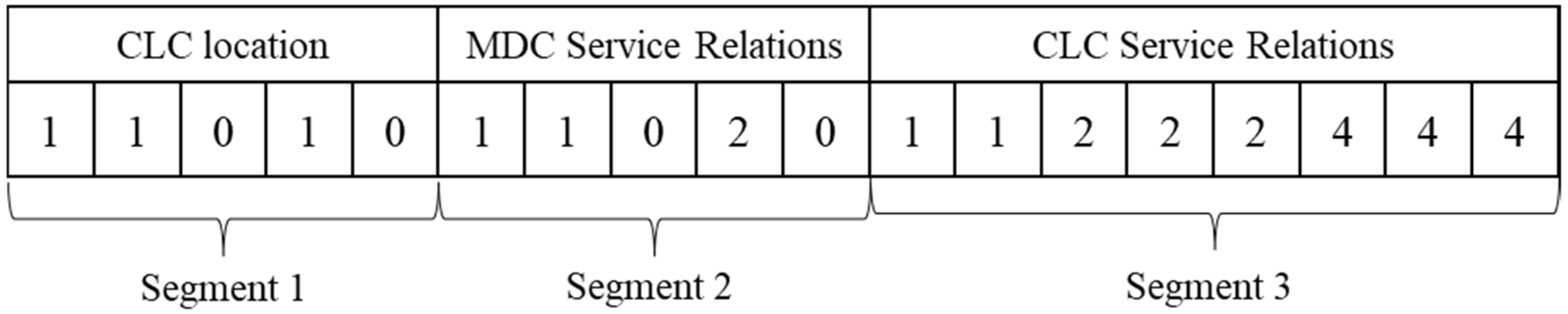
4.1. Chromosome Coding and Initial Population Generation

The EHR-NSGA-II designed in this study uses a segmented coding method. Each chromosome consists of $T$ substrings. $T$ is the number of periods in a large-scale project. Each substring corresponds to a CLC location–allocation scheme in a period. The substring can be split into three segments, and each genetic position in each segment corresponds to a decision variable. Segment 1 in the substring represents the location scheme of the CLC encoded in binary. The segment length is the number of potential CLCs. A genetic position with a value of 1 indicates that the CLC is open. Otherwise, it is 0. Segment 2 in the substring represents the service relationship between the CLC and the MDC and is encoded in real numbers. The length of segment 2 is the number of potential CLCs. Each genetic position takes values from 1 to $j$ ($j$ is the number of MDCs). Closed CLCs correspond to genes with meaningless values. Segment 3 in the substring represents the allocation relationship between the construction sections and CLCs and is encoded in real numbers. The length of segment 3 is the number of construction sections, and each genetic position takes values from 1 to $k$ ($k$ is the number of potential CLCs). The value of fragment 3 depends on the value of fragment 1. Only the genes in fragment 1 that take the value of 1 can be the values of the genes in fragment 3. This is because only the CLC in fragment 1 is open to provide material transport services for the construction sections in fragment 3.

Each chromosome is generated by randomly selecting $x$ CLCs open from $k$ potential CLCs. The service relationships between the CLC and the material distribution center and between the CLC and the construction bids are then determined based on the constraints. Subsequently, the chromosomes are checked to determine whether they satisfy the model’s constraints, and the chromosomes that violate the model constraints are repaired. The above methods randomly generate several chromosomes to form the parent population.

For example, a construction logistics network has two MDCs, five potential CLCs, and eight construction sections. Figure 3 illustrates a substring of chromosomes for a feasible solution. Segment 1 in the substring indicates the opening of CLCs numbered 1, 2, and 4. Segment 2 of the substring indicates that CLCs numbered 1 and 2 are provided with material transport services by MDC numbered 1. CLC number 4 is transported by MDC number 2. CLCs numbered 3 and 5 take meaningless values. Segment 3 in the substring indicates that construction sections numbered 1 and 2 are supplied by the CLC numbered 1. Construction sections numbered 3, 4, and 5 are provided by the CLC numbered 2. Construction sections numbered 5, 6, and 7 are supplied by the CLC numbered 4.

4.2. Fitness Calculation and Fast Non-Dominated Sorting

The fitness function of a genetic algorithm is usually equivalent to the model’s objective function. The fitness function in this paper’s algorithm is represented as a vector of two objectives: $F=\left(f_1,f_2\right)$. $f_1$ is the total cost, and $f_2$ is the total transportation risk.

Fast non-dominated sorting is a hierarchical processing method proposed by Deb in 2002 for sorting population dominance relations, which can effectively reduce the complexity of population non-dominated stratification [51]. Assume that every population has a number $n\left(i\right)$ of individuals that dominate it and a number $S\left(i\right)$ of individuals that are dominated by it. When $n\left(i\right)=0$, any other individual does not dominate it, and it is deposited in the first non-dominated layer. At the same time, $S\left(i\right)$ of all individuals in a set of individuals dominated by it is subtracted by 1 until all individuals are graded.

4.3. Dynamic Crowding Distance

Crowding distance reflects the density of individuals in the target space. The smaller the crowding distance is, the more dispersed the individuals are in the target space and the stronger the search ability is. However, in the traditional crowding distance calculation method, when individuals with low crowding distance are gathered in a specific region, the fixed crowding distance sorting strategy may eliminate all the individuals in that region, making the diversity of the finally obtained Pareto solution set worse. This paper adopts a dynamic crowding distance sorting strategy to overcome the shortcomings of the fixed crowding distance sorting method in practical applications. When the algorithm needs to eliminate the individual with the smallest crowding distance from the $h$ individuals in the $F_n$ layer of the population, the dynamic crowding distance sorting strategy is used. After eliminating an individual, the position $l$ of the individual is recorded, and the crowding distances of the individuals located in $l-1$ and $l+1$ are recalculated. The individual with the lowest crowding distance is removed based on the updated crowding distance ranking until the number of individuals in the population meets the requirement.

4.4. Binary Tournament Selection

The binary tournament selection process consists of randomly selecting two individuals at a time in the population and determining the dominant relationship between the two individuals. If there is a dominant relationship, then the better individual enters the next generation of the population. If no dominance relationship exists, then the crowding values are compared, and the one with the larger crowding value enters the next generation. This operation is repeated until the next-generation population consisting of the selected individuals is the same size as the original population. The binary tournament selection strategy facilitates parallelized processing and avoids falling into local optimal solutions. It ensures that the excellent individuals are copied into the next generation during the selection process of each generation, which accelerates the convergence speed of the algorithm [53].

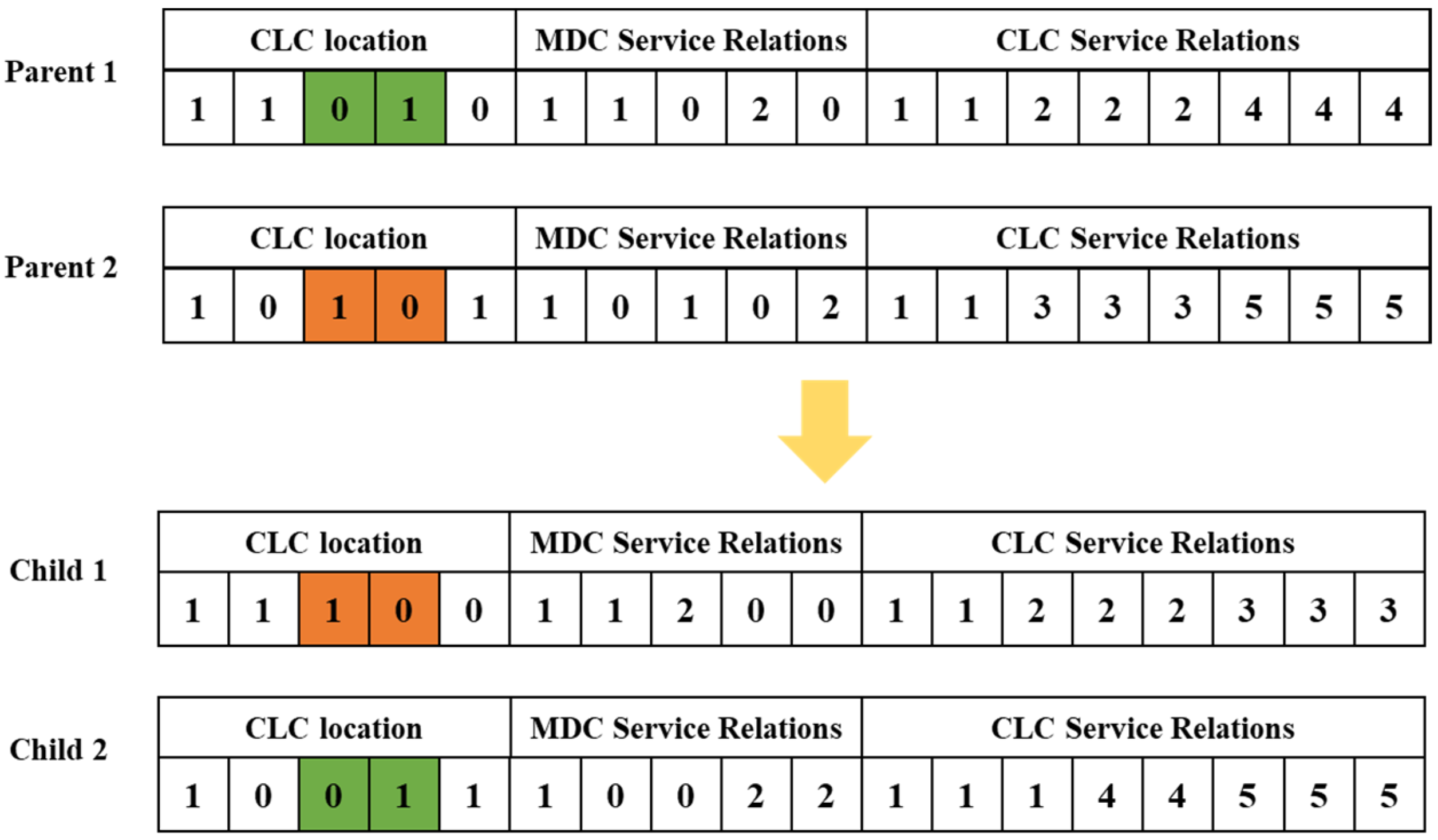
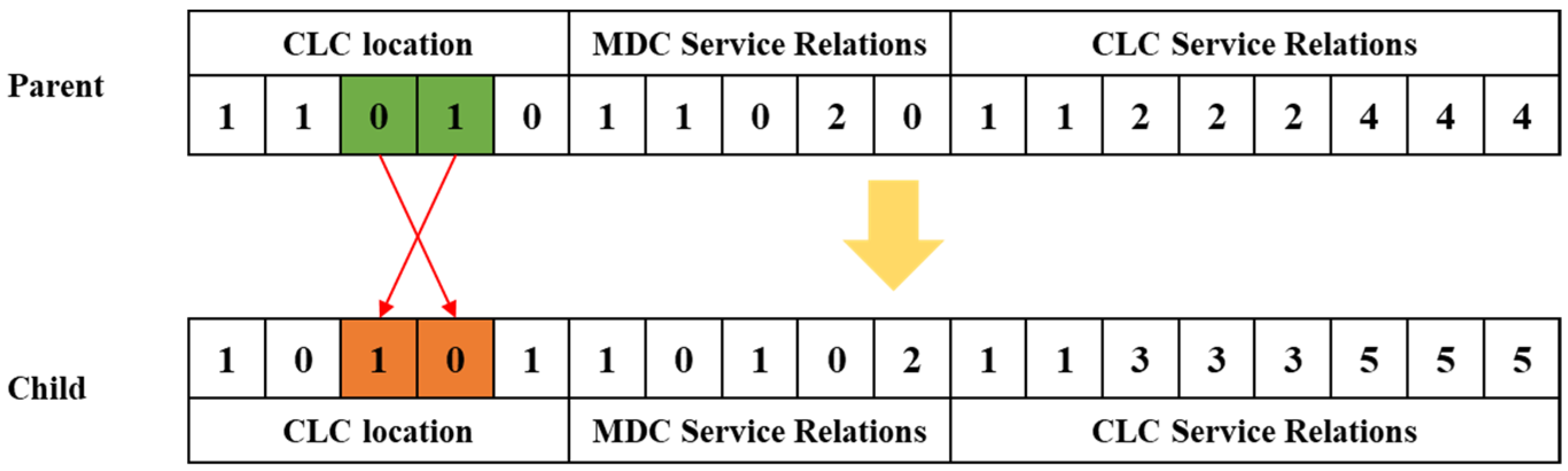
4.5. Crossover, Variational Operator Design

Genetic algorithms’ crossover and mutation probability are crucial in algorithm convergence and solution quality [54]. Increasing the crossover probability and decreasing the mutation probability in the early stage of population evolution is conducive to rapid convergence of the population, and the better solution is less likely to be lost. Lowering the crossover probability and increasing the mutation probability in the later stage of population evolution is conducive to fine-tuning the search for the optimal solution and maintaining the diversity of the population. However, the traditional genetic algorithm’s crossover probability and mutation probability are fixed, which leads to the deterioration of the optimization ability and optimization results of the genetic algorithm. Therefore, this paper draws on the mutual promotion and inhibition of hormone regulation so that the genetic algorithm’s crossover probability and mutation probability are adaptively adjusted according to the standard deviation of the fitness function value, to promote population diversity and overcome the problems of precocity and slow evolution of the genetic algorithm.

Farhy proposed the basic rules of endocrine hormones in 2004, revealing that hormones have monotonic and non-negative change characteristics [55]. The ascending regularity function $U_{up}\left(H\right)$ and the descending regularity function $U_{down}\left(H\right)$ of hormone regulation follow the $\mathrm{Hill}$ functional rules expressed in the formulas shown in (29) and (30).

$$U_{up}\left(H\right)={\displaystyle \frac{H^n}{O^n+H^n}}$$

(29)

$$U_{down}\left(H\right)={\displaystyle \frac{O^n}{O^n+H^n}}$$

(30)

where $H$ is the function independent variable. $O$ is the threshold value, and $O>0$. $N$ is the coefficient of the $\mathrm{Hill}$ function, and $\mathrm{N}\ge 1$. $N$ and $O$ together determine the slope of the upward and downward function curves.

If hormone $v$ is regulated by hormone $w$, the relationship between the secretion rate $S_v$ of hormone $v$ and the concentration $E_w$ of hormone $w$ is:

$$S_v=\alpha F\left(E_w\right)+S_{v0}$$

(31)

where $S_{v0}$ is the basal secretion rate of the hormone $v$, and $\alpha$ is a constant factor.

Substituting Equations (29) and (30) into Equation (31), Equations (32) and (33) are obtained.

$$P_{up}=\alpha {\displaystyle \frac{E_w^n}{O^n+E_w^n}}+S_{v0}=S_{v0}\left(1+{\displaystyle \frac{\alpha }{S_{v0}}}\times {\displaystyle \frac{E_w^n}{O^n+E_w^n}}\right)$$

(32)

$$P_{down}=\alpha {\displaystyle \frac{O_w^n}{O^n+E_w^n}}+S_{v0}=S_{v0}\left(1-{\displaystyle \frac{\alpha }{S_{v0}}}\times {\displaystyle \frac{E_w^n}{O^n+E_w^n}}\right)+\alpha$$

(33)

Corresponding to the genetic algorithm, the concentration $E_w$ of hormone $w$ is the number of algorithm iterations. Equation (32) is the formula for the rate of increase in the mutation probability. Equation (33) is the crossover probability falling rate formula.

After determining the crossover and mutation adaptive change probabilities, offspring are generated by crossover and mutation works. Specifically, we select the first chromosome segment as the basic chromosome. Crossover and mutation are performed only on the basic chromosome. This is because once the location of the CLC changes, its service relationship with the MDC and the construction section will change as well. After each crossover and mutation, the second and third segments of chromosomes are generated according to the constraints. Schematic diagrams of the crossover and mutation operations in this paper are shown in Figure 4 and Figure 5.

5. Result and Discussion

This section analyzes the performance of the models and algorithms using data from a large-scale railroad construction project in complex environmental regions. First, the model was coded and solved using MATLAB R2020b optimization software. The solution results of the multiperiod CLC location–allocation model designed in this paper were compared with those of the single-period model. The performance gap between the EHR-NSGA-II and other multi-objective algorithms was analyzed. Then, the square CLC location–allocation cases with different objective biases were given, and the costs and risks of various schemes were investigated. Finally, a sensitivity analysis of the critical parameters in the case was performed. All experiments were conducted on a computer with a 3.60 GHz CPU, 16 GB RAM, and an Intel^® Core ™ i7-9700 processor. The Intel chips come from Intel’s Chengdu factory in China.

5.1. Case Data Collection

The large-scale railroad construction project in the case study can be divided into five periods based on schedule planning. The duration of periods I to V is one year, one year, four years, two years, and two years, respectively, for a total of 10 years. Data on road transportation distances between the MDC, CLC, and construction sections were calculated by using Amap v15.06. Unit freight rates for different materials were collected by consulting with construction companies. Transportation road risk data between the MDC, CLC, and construction sections were calculated based on the dataset [56] and using ArcGIS 10.2 with a buffer set at a 3 km range of the transportation road. The main materials required for the construction sections of the project are steel, fly ash, and cement, with annual average storage costs of RMB 200/t, RMB 400/t, and RMB 100/t, respectively. Taking steel as an example, the average daily demand for different periods is shown in

Table 3. Average daily demand for steel in different periods for each construction section.

Number	Periodic Average Daily Demand (t)					Number	Periodic Average Daily Demand (t)
	I	II	III	IV	V		I	II	III	IV	V
1	43.9	73.1	73.1	43.9	/	17	/	9.9	16.5	16.5	9.9
2	25.2	42	42	25.2	/	18	/	25.2	42.1	42.1	25.2
3	8.5	14.2	14.2	8.5	/	19	/	21.8	36.3	36.3	21.8
4	95.3	158.8	158.8	95.3	/	20	/	11.1	18.6	18.6	11.1
5	43.3	72.1	72.1	43.3	/	21	/	21.9	36.4	36.4	21.9
6	/	48.6	81.0	81.0	48.6	22	/	8.5	14.1	14.1	8.5
7	/	17.3	28.8	28.8	17.3	23	/	21.1	35.2	35.2	21.1
8	/	19.7	32.9	32.9	19.7	24	/	7.6	12.7	12.7	7.6
9	/	33.5	55.8	55.8	33.5	25	9	15.1	15.1	9	/
10	/	26	43.4	43.4	26	26	4.6	7.6	7.6	4.6	/
11	/	20.4	33.9	33.9	20.4	27	19.1	31.8	31.8	19.1	/
12	/	16	26.6	26.6	16	28	14.1	23.5	23.5	14.1	/
13	/	14.7	24.4	24.4	14.7	29	12.7	21.2	21.2	12.7	/
14	/	4	6.7	6.7	4	30	13.2	22	22	13.2	/
15	/	24.7	41.2	41.2	24.7	31	10.3	17.1	17.1	10.3	/
16	/	15.4	25.7	25.7	15.4	32	10.6	17.7	17.7	10.6	/

.

In seasons when transport road disruptions occur less frequently, the safety stock period for the CLC is generally set at 15 days. During seasons when transport road disruptions are more frequent, the safe stocking period of the CLC will be increased appropriately. If a CLC is to be opened, it must provide material transport and storage services for at least two construction sections. Therefore, in general, the minimum stock utilization rate is set at 0.4, which means that the service requirements of two construction sections are met. Through communication with the project design unit, the cost and storage capacity information related to the potential CLC in the case is shown in

Table 4. Data related to potential CLC.

Potential CLC Number	Area (mu 1)	Potential CLC-Related Unit Costs (RMB/mu)				Capacity Ceiling (t)
		Construction	Opening	Fixed Operating	Closing	Steel	Fly Ash	Cement
1	50	200,000	30,000	80,000	60,000	10,000	100,000	12,000
2	40	200,000	30,000	80,000	60,000	8000	80,000	9600
3	30	300,000	40,000	100,000	80,000	6000	60,000	7200
4	40	300,000	50,000	100,000	80,000	8000	80,000	9600
5	40	300,000	50,000	120,000	80,000	8000	80,000	9600
6	35	350,000	50,000	120,000	90,000	7000	70,000	8400
7	45	500,000	60,000	150,000	90,000	9000	90,000	10,800
8	45	500,000	60,000	150,000	100,000	9000	90,000	10,800
9	40	500,000	60,000	160,000	120,000	8000	80,000	9600
10	45	500,000	70,000	160,000	120,000	9000	90,000	10,800
11	50	500,000	70,000	160,000	140,000	10,000	100,000	12,000
12	40	300,000	60,000	140,000	90,000	8000	80,000	9600
13	50	300,000	50,000	120,000	80,000	10,000	100,000	12,000

¹ A Chinese unit of land measurement that is commonly 666.7 square meters.

.

5.2. Model and Algorithm Performance Analysis

5.2.1. Model Performance Analysis

To analyze the performance of the multiperiod CLC location–allocation model, the results of the multiperiod model solution are compared with those of the single-period model solution. Because the results obtained from the direct solution of the multi-objective model are Pareto solution sets, it is not convenient to compare the model performance. Therefore, before solving the model, this paper transforms the multi-objective model into a single-objective model using the weighted average sum method. The solution results of different models are shown in

Table 5. Single-period and multiperiod model solution results.

Modeling Objective	Single-Period Model	Multiperiod Model
Transportation costs (RMB)	2.55 × 1010	2.55 × 1010
Construction cost (RMB)	7.35 × 107	9.7 × 107
Opening cost (RMB)	1.03 × 107	1.29 × 107
Closing cost (RMB)	1.94 × 107	2.81 × 107
Operating cost (RMB)	3.28 × 108	1.19 × 108
Warehousing cost (RMB)	1.58 × 107	1.57 × 107
Total cost (RMB)	2.59 × 1010	2.38 × 1010
Risk factor	5,275,545	4,794,092

.

As shown in Table 5, compared with the single-period model solution result, the total cost in the multiperiod model solution result is reduced by 8.11%. For each cost, because the multiperiod model considers the periodic construction material demand changes, the CLC can be constructed, opened, or closed at a suitable time in response to construction material demands. As a result, the transportation cost in the multiperiod model solution is reduced by 7.84%, and the operation cost is reduced by 63.72%.

5.2.2. Algorithm Performance Analysis

To analyze the performance of the EHR-NSGA-II algorithm, NSGA-II [51], ARSBX-NSGA-II [57], and NSGA-III [58] were selected to address the case problem using the same number of iterations. The values of the algorithm parameters are shown in

Table 6. Algorithm parameter values.

Parameters	Value	Parameters	Value
$O$	1	$n$	2
$S_{v0}$	2	Population size	50
Initial crossover probability	0.6	Iterations	500
Initial mutation probability	0.05

, where the parameters related to the endocrine hormone regulatory function are referred to in the article of [59]. The Pareto solution set for the four multi-objective algorithms is shown in Figure 6.

As shown in Figure 6, all four multi-objective algorithms can address the CLC location–allocation problem for multiperiod railroad projects. However, the Pareto solution set curve generated by the EHR-NSGA-II algorithm designed in this paper is smoother and more evenly distributed. Meanwhile, the single-objective optimal values in the Pareto optimal solutions of the four multi-objective algorithms are counted, and the results are shown in

Table 7. Different algorithms result in single-objective optimal values.

Objective	EHR-NSGA-II	NSGA-II	NSGA-II-ARSBX	NSGA-III
Total Cost (RMB)	1.93 × 1010	2.32 × 1010	2.25 × 1010	2.56 × 1010
Gap	/	16.8%	14.2%	24.6%
Risk factor	4,191,693	4,678,358	4,220,307	4,271,501
Gap	/	10.4%	0.7%	1.9%

. The single-objective optimal values obtained by the EHR-NSGA-II algorithm designed in this paper are smaller than those obtained by the other three algorithms, indicating that EHR-NSGA-II can better find the optimal values.

To further assess the diversity of the Pareto solution sets, the number of Pareto solutions, the spread metric [60], and the spacing metric [61] were used to evaluate the Pareto solution sets obtained using different algorithms. Spacing and spread measure the distribution of the solution sets generated by the algorithms. Spacing measures the minimum Euclidean distance between all solutions, which can evaluate the uniformity of the spatial distribution of the solution sets. The smaller the value of spacing is, the more uniform is the distribution of the solution sets. Spread measures the maximum Euclidean distance between all solutions, which can evaluate the breadth of the solution set space. The larger the value of spread is, the broader is the distribution of the solution set space. The diversity assessment results of the Pareto solution sets of different algorithms are shown in

Table 8. Metrics for evaluating the diversity of the Pareto solution sets for different algorithms.

Evaluation Indicators	EHR-NSGA-II	NSGA-II	NSGA-II-ARSBX	NSGA-III
Pareto solution quantity	18	7	13	10
Gap	/	157.1%	38.5%	80%
Spread	6.56 × 109	6.49 × 108	3.1 × 109	2.25 × 109
Gap	/	910.8%	111.6%	191.6%
Spacing	1.81 × 107	2.03 × 107	3.96 × 107	6.32 × 107
Gap	/	10.8%	54.3%	71.4%

.

As shown in Table 8, the solution set obtained by EHR-NSGA-II designed in this study is better than the solution sets obtained by the other three algorithms in terms of the number of Pareto solutions, uniformity of the solution set space, and extensiveness. In summary, EHR-NSGA-II addresses multiperiod CLC location–allocation problems more effectively.

5.3. Results Analysis

Compared with the weighted square and multi-objective optimization methods, EHR-NSGA-II can simultaneously consider multiple objectives of the model. Solutions satisfying various needs are obtained in one calculation, which provides sufficient choice space for the decision maker and effectively improves the optimization decision level.

Table 9. EHR-NSGA-II Pareto solution set.

No.	Total Cost	Risk Factor	No.	Total Cost	Risk Factor	No.	Total Cost	Risk Factor
1	1.93 × 1010	5,981,568	7	2.03 × 1010	5,335,713	13	2.30 × 1010	4,743,494
2	1.97 × 1010	5,869,065	8	2.05 × 1010	5,215,202	14	2.34 × 1010	4,617,659
3	1.98× 1010	5,709,204	9	2.06 × 1010	5,202,250	15	2.37 × 1010	4,596,207
4	1.98 × 1010	5,572,658	10	2.1 × 1010	5,071,215	16	2.40 × 1010	4,440,042
5	1.99 × 1010	5,508,576	11	2.15 × 1010	4,973,909	17	2.42 × 1010	4,417,647
6	2.02 × 1010	5,355,170	12	2.26 × 1010	4,862,238	18	2.59 × 1010	4,191,694

shows the Pareto solution set obtained by solving the EHR-NSGA-II algorithm.

This paper selected three representative solutions from the Pareto solution set obtained by solving EHR-NSGA-II, as shown in

Table 10. Typical solutions of the EHR-NSGA-II algorithm.

Objectives	Scheme I	Scheme II	Scheme III
Transportation costs (RMB)	1,898,816	2,556,901	2,120,308
Construction cost (RMB)	10,450	9700	9550
Opening cost (RMB)	1600	1585	1420
Closing cost (RMB)	2820	2685	2505
Operating cost (RMB)	13,960	12,600	12,460
Warehousing cost (RMB)	1576	1576	1576
Total cost (RMB)	1,929,222	2,585,048	2,403,886
Risk factor	5,981,568	4,191,694	4,440,042

. Scheme I is the minimum cost solution that can satisfy the decision maker when pursuing the lowest total cost. Scheme II is the minimum risk solution, which can meet decision makers’ needs when pursuing the minimum risk of construction logistics transportation. Scheme III is a compromise solution between the two objectives, which can satisfy the decision maker’s need to balance the minimization of total cost and the minimization of transportation risk.

As shown in Table 10, transportation costs account for more than 90% of the total costs due to the long construction duration. The total cost of the construction logistics network and the transportation risk have a mutually constraining relationship. As the total cost gradually increases, the transportation risk for construction materials gradually decreases. However, in scheme III, which considers the total cost and transportation risk, the construction, opening, and closing costs of the construction logistics network are the lowest. This indicates that the compromise scheme can better use the constructed CLC. The remaining two schemes involve the excessive construction of CLCs to reduce cost or transportation risks.

The location–allocation schemes for CLCs under the five different periods of scheme III are shown in Figure 7. Only three CLCs were open in the first period, because only some construction sections had begun. The number of open CLCs increased gradually as more construction sections start construction and the construction material demand increases. In the third cycle, the construction material demand for each construction section peaked, and the number of CLCs increased to six. The number of CLCs then decreased as the construction material demand decreased. In the last period, the number of CLCs decreased to three. During the change in the number of CLCs, the service relationship of the construction sections also changed because of distance, capacity constraints, and transportation risks.

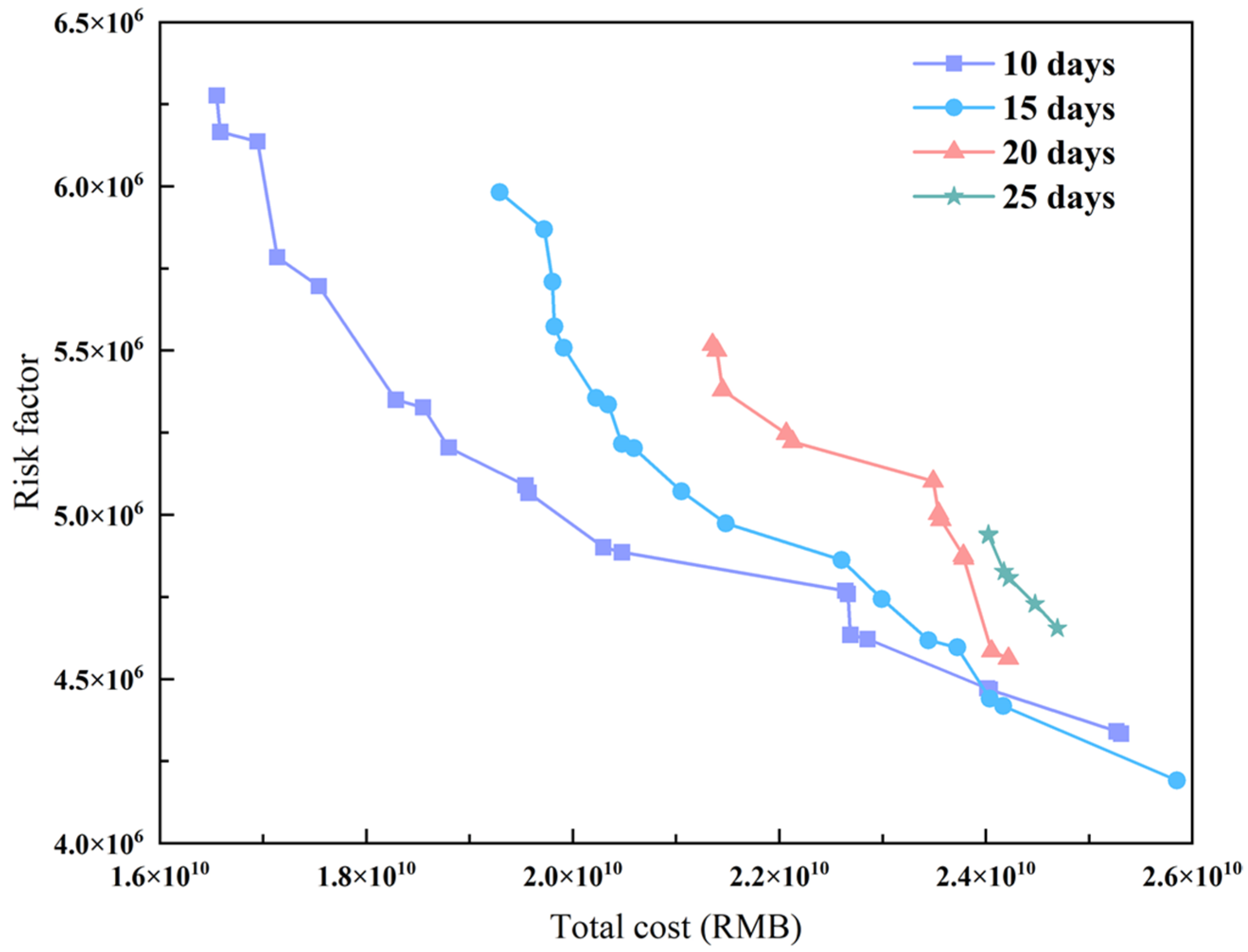
5.4. Sensitivity Analysis

Finally, this paper conducted a parametric sensitivity analysis of the multiperiod railroad project CLC siting model. The effects of coverage and safety stock period on total cost as well as risk factors were explored.

5.4.1. Coverage Sensitivity Analysis

The safety stock period has been set to take the value of 15 days, and the coverage range has taken the values of 400, 800, and 1200 km. The Pareto solution set obtained using EHR-NSGA-II is shown in Figure 8.

As shown in Figure 8, with the coverage decreasing, the Pareto solution set shifts from the lower left to the upper right, and the total cost and risk coefficients gradually increase. This indicates that when the coverage range is small, construction sections are forced to choose a CLC at a higher cost and risk due to the service distance constraint. As the coverage range value increases, the choice of CLC site selection and construction section allocation also widens. Construction sections can choose CLCs with lower cost and risk to provide construction material transportation services for them. Thus, the construction logistics network’s total cost and risk factors gradually decrease. However, regarding the increase in total cost and risk factor, the increase in the coverage distance from 800 to 400 km is more significant than that from 1200 to 800 km. This indicates that the effect of the increase in total cost and risk coefficient with the decrease in the coverage range has a gradually increasing trend.

5.4.2. Safety Stock Period Sensitivity Analysis

The coverage area was set to take the value of 800 km and the safety stock period to take the values of 10, 15, 20, and 25 days. The Pareto solution set obtained using EHR-NSGA-II is shown in Figure 9.

As shown in Figure 9, as the safety stock period increases, the quality of the solutions gradually decreases, and the number of Pareto solutions decreases substantially. When the safety stock period is over 25 days, a feasible solution that satisfies the model constraints cannot be found. According to the distribution of the Pareto solution sets under different safety stock periods, when the total cost is the same, the risk factor of Pareto solutions with more considerable safety stock periods is higher. When the risk coefficients are the same, the total cost of the Pareto solution set with a more considerable safety stock period is higher. This suggests that when the safety stock period is more considerable, construction sections are forced to choose the CLC with a higher cost and transportation risk because of the constraints of the CLC inventory capacity. As the safety inventory period decreases, the choice of CLC location and the allocation of construction sections become more expansive, and the quality of the Pareto solution set gradually improves. In summary, although increasing the safety stock period can effectively prevent shortages of construction sections, it affects the overall cost and transportation safety of the construction logistics network.

5.5. Managerial Insights

The results of the case studies in this paper can provide some critical management insights and practical implications. First, given the cost reduction potential of the proposed CLC multiperiod location–allocation scheme, managers have the flexibility to establish CLC construction, opening, and closing plans based on the project schedule. This will not only avoid the pressure on the transport network caused by the construction of many CLCs at the same time but will also reduce the operating costs of the CLCs. Meanwhile, as the sensitivity analyses demonstrated, variations in the safety stock period play an essential role in developing CLC construction schemes. Therefore, managers should reasonably set the safety stock period based on measuring the transport risk of practical application scenarios, which can reduce the cost of CLC construction and operation and the risk of material transport. Second, in the context of the continuous emphasis on reliability and punctuality of construction material transportation, both suppliers and construction sections want to achieve JIT transportation of construction materials. However, the analyses in this paper also strongly confirm the significant cost impact of service radius constraints. Reducing the CLC service radius to improve the timeliness of transportation for construction materials will inevitably increase the total cost. Therefore, managers should appropriately ease the time requirement for transporting construction materials to reduce logistics costs and ensure construction sections’ regular operation.

6. Conclusions

This study considers large-scale CLC location and construction section service allocation as two major strategic decisions. First, a multi-objective, multiperiod, and multi-materials generic MPFLP model is designed to optimize the construction logistics network of large-scale projects, such as railroads, highways, and hydropower stations, to satisfy the decision maker’s requirements for cost and risk. In addition, the EHR-NSGA-II algorithm is designed to construct a building logistics network for an authentic railroad construction project. The effectiveness of the model and that of the algorithm are also compared and analyzed. Finally, the sensitivity of the model’s key parameters is analyzed, and the influence of the parameter values on the model is discussed.

Algorithm effectiveness analysis shows that compared with NSGA-II, ARSBX-NSGA-II, and NSGA-III, the EHR-NSGA-II designed in this study outperforms the other three algorithms in terms of optimality finding ability, the number of Pareto solutions, and the uniformity and extensiveness of the distribution of the Pareto solution sets. The model effectiveness analysis shows that the multiperiod model designed in this paper reduces the total cost by 8.11% compared with the single-period model, which reduces the operating cost by 63.72%. The applicability and effectiveness of the model for large-scale construction logistics network optimization problems are demonstrated. The sensitivity analysis shows that the proposed model is more sensitive to the safety stock period value than the coverage. An excessively high safety stock period value will significantly increase the cost of the engineering logistics network. In summary, the multiperiod construction logistics network optimization model and the EHR-NSGA-II algorithm designed in this paper can help managers construct efficient and robust construction logistics networks based on careful consideration of cost and risk.

However, this paper still has some limitations. In the process of model construction, this paper considers the risk of construction material transport and periodic changes in demand but fails to construct the model from the perspective of uncertainty. During the operation of construction logistics networks in complex environment regions, road interruption is often caused by unexpected events, which leads to changes in material transport time and transport cost. At the same time, geological disasters and changes in construction plans also lead to changes in the demand for construction materials. These uncertainties are important factors affecting the optimization of construction logistics networks. If stochastic optimization or robust optimization is used to portray these uncertainties, the destruction resistance of the construction logistics network will be significantly improved. In addition, due to the limitation of the fixed capacity of the CLC, the adjustment of the safety stock period seriously affects the number of Pareto solutions. In the future, capacity-variable models can be constructed to overcome the problem of decreasing feasible solutions due to an increase in the safety stock period.

References

1. Fredriksson, A.; Janné, M.; Rudberg, M. Characterizing third-party logistics setups in the context of construction. Int. J. Phys. Distrib. Logist. Manag. 2021, 51, 325–349. [Google Scholar] [CrossRef]
2. Ahmadian, F.F.A.; Akbarnezhad, A.; Rashidi, T.H.; Waller, S.T. Accounting for Transport Times in Planning Off-Site Shipment of Construction Materials. J. Constr. Eng. Manag. 2016, 142, 04015050. [Google Scholar] [CrossRef]
3. Tetik, M.; Peltokorpi, A.; Seppänen, O.; Leväniemi, M.; Holmström, J. Kitting Logistics Solution for Improving On-Site Work Performance in Construction Projects. J. Constr. Eng. Manag. 2021, 147, 05020020. [Google Scholar] [CrossRef]
4. Fallahnejad, M.H. Delay causes in Iran gas pipeline projects. Int. J. Proj. Manag. 2013, 31, 136–146. [Google Scholar] [CrossRef]
5. Guerlain, C.; Renault, S.; Ferrero, F. Understanding Construction Logistics in Urban Areas and Lowering Its Environmental Impact: A Focus on Construction Consolidation Centres. Sustainability 2019, 11, 6118. [Google Scholar] [CrossRef]
6. Josephson, P.-E.; Saukkoriipi, L. Waste in Construction Projects: Call for a New Approach; 9197618179; Chalmers University of Technology: Gothenburg, Sweden, 2007. [Google Scholar]
7. Zeng, L.; Du, Q.; Zhou, L.; Wang, X.; Zhu, H.; Bai, L. Side-payment contracts for prefabricated construction supply chain coordination under just-in-time purchasing. J. Clean. Prod. 2022, 379, 134830. [Google Scholar] [CrossRef]
8. Yao, J.; Yi, W.; Wang, H.; Zhen, L.; Liu, Y. Stackelberg game model for construction waste disposal network design. Autom. Constr. 2022, 144, 104573. [Google Scholar] [CrossRef]
9. Sundquist, V.; Gadde, L.E.; Hulthén, K. Reorganizing construction logistics for improved performance. Constr. Manag. Econ. 2018, 36, 49–65. [Google Scholar] [CrossRef]
10. Hedborg Bengtsson, S. Coordinated construction logistics: An innovation perspective. Constr. Manag. Econ. 2018, 37, 294–307. [Google Scholar] [CrossRef]
11. Dubois, A.; Gadde, L.-E. The construction industry as a loosely coupled system: Implications for productivity and innovation. Constr. Manag. Econ. 2002, 20, 621–631. [Google Scholar] [CrossRef]
12. Dubois, A.; Hulthén, K.; Sundquist, V. Organising logistics and transport activities in construction. Int. J. Logist. Manag. 2019, 30, 620–640. [Google Scholar] [CrossRef]
13. El Moussaoui, S.; Lafhaj, Z.; Leite, F.; Laqdid, Y.; BuHamdan, S.; Brunet, F.; Fléchard, J.; Linéatte, B. The Assessment of Pollutant Emissions from Transportation of Construction Materials and the Impact of Construction Logistics Centers. J. Manag. Eng. 2022, 38, 04022038. [Google Scholar] [CrossRef]
14. Dakhli, Z.; Lafhaj, Z. Considering Materials Management in Construction: An Exploratory Study. Logistics 2018, 2, 7. [Google Scholar] [CrossRef]
15. Sezer, A.A.; Fredriksson, A. Environmental impact of construction transport and the effects of building certification schemes. Resour. Conserv. Recycl. 2021, 172, 105688. [Google Scholar] [CrossRef]
16. Janné, M.; Fredriksson, A. Construction logistics governing guidelines in urban development projects. Constr. Innov. 2019, 19, 89–109. [Google Scholar] [CrossRef]
17. El Moussaoui, S.; Lafhaj, Z.; Leite, F.; Fléchard, J.; Linéatte, B. Construction Logistics Centres Proposing Kitting Service: Organization Analysis and Cost Mapping. Buildings 2021, 11, 105. [Google Scholar] [CrossRef]
18. Shafiei Kisomi, M.; Solimanpur, M.; Doniavi, A. An integrated supply chain configuration model and procurement management under uncertainty: A set-based robust optimization methodology. Appl. Math. Modell. 2016, 40, 7928–7947. [Google Scholar] [CrossRef]
19. Amiri, A. Designing a distribution network in a supply chain system: Formulation and efficient solution procedure. Eur. J. Oper. Res. 2006, 171, 567–576. [Google Scholar] [CrossRef]
20. Hsu, P.-Y.; Angeloudis, P.; Aurisicchio, M. Optimal logistics planning for modular construction using two-stage stochastic programming. Autom. Constr. 2018, 94, 47–61. [Google Scholar] [CrossRef]
21. Azambuja, M.; O’Brien, W.J. Supply chain modeling: Issues and perspectives. In Construction Supply Chain Management Handbook; CRC: Boca Raton, FL, USA, 2008. [Google Scholar]
22. Lei, L.; Liu, S.; Ruszczynski, A.; Park, S. On the integrated production, inventory, and distribution routing problem. IIE Trans. (Inst. Ind. Eng.) 2006, 38, 955–970. [Google Scholar] [CrossRef]
23. Said, H.; El-Rayes, K. Optimizing Material Procurement and Storage on Construction Sites. J. Constr. Eng. Manag. 2011, 137, 421–431. [Google Scholar] [CrossRef]
24. Li, J.Q.; Han, Y.Q.; Duan, P.Y.; Han, Y.Y.; Niu, B.; Li, C.D.; Zheng, Z.X.; Liu, Y.P. Meta-heuristic algorithm for solving vehicle routing problems with time windows and synchronized visit constraints in prefabricated systems. J. Clean. Prod. 2020, 250, 119464. [Google Scholar] [CrossRef]
25. RezaHoseini, A.; Noori, S.; Ghannadpour, S.F. Integrated scheduling of suppliers and multi-project activities for green construction supply chains under uncertainty. Autom. Constr. 2021, 122, 103485. [Google Scholar] [CrossRef]
26. Guerra, B.C.; Shahi, S.; Molleai, A.; Skaf, N.; Weber, O.; Leite, F.; Haas, C. Circular economy applications in the construction industry: A global scan of trends and opportunities. J. Clean. Prod. 2021, 324, 129125. [Google Scholar] [CrossRef]
27. Lundesjo, G.T.L. Using Construction Consolidation Centres to Reduce Construction Waste and Carbon Emissions; Waste & Resources Action Programme: Banbury, UK, 2011; pp. 1–19. [Google Scholar]
28. Ding, L.; Wang, T.; Chan, P.W. Forward and reverse logistics for circular economy in construction: A systematic literature review. J. Clean. Prod. 2023, 388, 135981. [Google Scholar] [CrossRef]
29. Lundesjö, G. Supply Chain Management and Logistics in Construction: Delivering Tomorrow’s Built Environment; Kogan Page Publishers: London, UK, 2015. [Google Scholar]
30. El-Anwar, O.; Kim, Y.W. Multi-objective optimization of process design using process-based sustainable impact analysis. In Proceedings of the EG-ICE 2010—17th International Workshop on Intelligent Computing in Engineering, Enschede, The Netherlands, 6–8 July 2011. [Google Scholar]
31. Fang, Y.; Ng, S.T. Genetic algorithm for determining the construction logistics of precast components. Eng. Constr. Arch. Manag. 2019, 26, 2289–2306. [Google Scholar] [CrossRef]
32. Xu, J.; Gang, J. Multi-objective bilevel construction material transportation scheduling in large-scale construction projects under a fuzzy random environment. Transp. Plan. Technol. 2013, 36, 352–376. [Google Scholar] [CrossRef]
33. Hsu, P.-Y.; Aurisicchio, M.; Angeloudis, P. Risk-averse supply chain for modular construction projects. Autom. Constr. 2019, 106, 102898. [Google Scholar] [CrossRef]
34. Ebrahimi-Zade, A.; Hosseini-Nasab, H.; Zare-Mehrjerdi, Y.; Zahmatkesh, A. Multi-period hub set covering problems with flexible radius: A modified genetic solution. Appl. Math. Modell. 2016, 40, 2968–2982. [Google Scholar] [CrossRef]
35. Canel, C.; Khumawala, B.M.; Law, J.; Loh, A. An algorithm for the capacitated, multi-commodity multi-period facility location problem. Comput. Oper. Res. 2001, 28, 411–427. [Google Scholar] [CrossRef]
36. Campbell, J.F. Locating transportation terminals to serve an expanding demand. Transp. Res. Part B Methodol. 1990, 24, 173–192. [Google Scholar] [CrossRef]
37. Gelareh, S. Hub Location Models in Public Transport Planning; VDM Verlag: Riga, Latvia, 2008. [Google Scholar]
38. Fattahi, P.; Kebria, Z.S. A bi-objective dynamic reliable hub location problem with congestion effects. Int. J. Ind. Eng. Prod. Res. 2020, 31, 63–74. [Google Scholar] [CrossRef]
39. Contreras, I.; Cordeau, J.F.; Laporte, G. The Dynamic Uncapacitated Hub Location Problem. Transp. Sci. 2011, 45, 18–32. [Google Scholar] [CrossRef]
40. Alumur, S.A.; Nickel, S.; Saldanha-da-Gama, F.; Seçerdin, Y. Multi-period hub network design problems with modular capacities. Ann. Oper. Res. 2016, 246, 289–312. [Google Scholar] [CrossRef]
41. Fotuhi, F.; Huynh, N. A reliable multi-period intermodal freight network expansion problem. Comput. Ind. Eng. 2018, 115, 138–150. [Google Scholar] [CrossRef]
42. Wang, X.-F.; Sun, X.-M.; Fang, Y. Genetic algorithm solution for multi-period two-echelon integrated competitive/uncompetitive facility location problem. Asia-Pac. J. Oper. Res. 2008, 25, 33–56. [Google Scholar] [CrossRef]
43. Khosravian, Y.; Shahandeh Nookabadi, A.; Moslehi, G. Mathematical Model for Bi-objective Maximal Hub Covering Problem with Periodic Variations of Parameters. Int. J. Eng. 2019, 32, 964–975. [Google Scholar] [CrossRef]
44. Reddy, K.N.; Kumar, A.; Choudhary, A.; Cheng, T.C.E. Multi-period green reverse logistics network design: An improved Benders-decomposition-based heuristic approach. Eur. J. Oper. Res. 2022, 303, 735–752. [Google Scholar] [CrossRef]
45. Bashiri, M.; Rezanezhad, M.; Tavakkoli-Moghaddam, R.; Hasanzadeh, H. Mathematical modeling for a p-mobile hub location problem in a dynamic environment by a genetic algorithm. Appl. Math. Modell. 2018, 54, 151–169. [Google Scholar] [CrossRef]
46. Goodarzian, F.; Wamba, S.F.; Mathiyazhagan, K.; Taghipour, A. A new bi-objective green medicine supply chain network design under fuzzy environment: Hybrid metaheuristic algorithms. Comput. Ind. Eng. 2021, 160, 107535. [Google Scholar] [CrossRef]
47. Ghaderi, A.; Jabalameli, M.S. Modeling the budget-constrained dynamic uncapacitated facility location–network design problem and solving it via two efficient heuristics: A case study of health care. Math. Comput. Modell. 2013, 57, 382–400. [Google Scholar] [CrossRef]
48. Wan, M.; Ye, C.; Peng, D. Multi-period dynamic multi-objective emergency material distribution model under uncertain demand. Eng. Appl. Artif. Intell. 2023, 117, 105530. [Google Scholar] [CrossRef]
49. Delfani, F.; Samanipour, H.; Beiki, H.; Yumashev, A.V.; Akhmetshin, E.M. A robust fuzzy optimisation for a multi-objective pharmaceutical supply chain network design problem considering reliability and delivery time. Int. J. Syst. Sci. Oper. Logist. 2022, 9, 155–179. [Google Scholar] [CrossRef]
50. Li, K.; Li, D.; Wu, D.Q. Carbon Transaction-Based Location-Routing-Inventory Optimization for Cold Chain Logistics. Alex. Eng. J. 2022, 61, 7979–7986. [Google Scholar] [CrossRef]
51. Giusti, R.; Manerba, D.; Tadei, R. Multiperiod transshipment location–allocation problem with flow synchronization under stochastic handling operations. Networks 2021, 78, 88–104. [Google Scholar] [CrossRef]
52. Deb, K.; Pratap, A.; Agarwal, S.; Meyarivan, T. A fast and elitist multiobjective genetic algorithm: NSGA-II. IEEE Trans. Evol. Comput. 2002, 6, 182–197. [Google Scholar] [CrossRef]
53. Huang, X.; Zong, J.; Wang, Q.; Liu, Y.; Wang, J.; Chen, P. Placement Approach for the Data Storage Management Function in a RAN-CN Converged Network. IEEE Access 2023, 11, 94898–94910. [Google Scholar] [CrossRef]
54. Almansour, F.M.; Alroobaea, R.; Ghiduk, A.S. An Empirical Comparison of the Efficiency and Effectiveness of Genetic Algorithms and Adaptive Random Techniques in Data-Flow Testing. IEEE Access 2020, 8, 12884–12896. [Google Scholar] [CrossRef]
55. Farhy, L.S. Modeling of Oscillations in Endocrine Networks with Feedback. In Methods Enzymology; Academic Press: Cambridge, MA, USA, 2004; Volume 384, pp. 54–81. [Google Scholar]
56. Zhang, Q.; Zhou, Q.; Wu, W.; Zhao, J.; Yuan, R. Hengduan Mountain Area Natural Disaster Risk and Comprehensive Risk Assessment Data Set (2020); National Tibetan Plateau/Third Pole Environment Data Center: Tibetan, China, 2021. [Google Scholar] [CrossRef]
57. Pan, L.Q.; Xu, W.T.; Li, L.H.; He, C.; Cheng, R. Adaptive simulated binary crossover for rotated multi-objective optimization. Swarm Evol. Comput. 2021, 60, 100759. [Google Scholar] [CrossRef]
58. Deb, K.; Jain, H. An Evolutionary Many-Objective Optimization Algorithm Using Reference-Point-Based Nondominated Sorting Approach, Part I: Solving Problems with Box Constraints. IEEE Trans. Evol. Comput. 2014, 18, 577–601. [Google Scholar] [CrossRef]
59. Kun, Z.; Zhiwei, L.; Yuguo, W.; Changjian, Z.; Xinyan, G.; Xuan, L. Improved Hormone Algorithm for Solving the Permutation Flow Shop Scheduling Problem. J. Univ. Electron. Sci. Technol. China 2022, 51, 890–903. [Google Scholar]
60. Wang, Y.N.; Wu, L.H.; Yuan, X.F. Multi-objective self-adaptive differential evolution with elitist archive and crowding entropy-based diversity measure. soft Comput. 2010, 14, 193–209. [Google Scholar] [CrossRef]
61. Wu, J.; Azarm, S. Metrics for Quality Assessment of a Multiobjective Design Optimization Solution Set. J. Mech. Des. 2000, 123, 18–25. [Google Scholar] [CrossRef]
Figure 1. Schematic diagram of multiperiod construction logistics network operation mode.
Buildings 15 01045 g001
Figure 2. Procedure of the EHR-NSGA-II.
Buildings 15 01045 g002
Figure 3. Schematic diagram of a substring of chromosomes for a feasible solution.
Buildings 15 01045 g003
Figure 4. Schematic diagram of crossover operation.
Buildings 15 01045 g004
Figure 5. Schematic diagram of the mutation operation.
Buildings 15 01045 g005
Figure 6. Distribution of the Pareto solution sets for four multi-objective algorithms.
Buildings 15 01045 g006
Figure 7. Schematic of the CLC location–allocation results for scheme III.
Buildings 15 01045 g007
Figure 8. Schematic of the Pareto solution set for different coverage areas.
Buildings 15 01045 g008
Figure 9. Schematic of the Pareto solution set over different safety stock periods.
Buildings 15 01045 g009