Abstract
With the continuous development of economic globalization, the research demand for intelligent agricultural machinery equipment in modern agriculture is increasing. This paper, which aims at the positioning problem of mobile robots in agriculture production, proposes a low-cost magnetic positioning scheme for cement ground. First, the analytical magnetic field model of ground magnets was established. Then, by comparing the analytic computing results, simulation results, and measured values, the modified model of magnetic fields was built and the relevant impact factors were calculated. After that, acquisition devices were used to collect the ground magnetic field data for the establishment of a magnetic field matching algorithm. Finally, the result showed that the positioning displacement error was ±1 mm, and the positioning accuracy was higher than the conventional indoor positioning method, which solved the problem of the low indoor positioning accuracy of agriculture mobile robots and contributes to the efficient production and modernization of agricultural machinery equipment.
1. Introduction
Mobile robots are a key enabling technology for applications in agricultural production [1]. Scholars are currently combining robotics with data science and control engineering to further improve reliability and practicality in planting and harvesting. Agricultural mobile robots require high positioning precision at the essential working position. It performs regular movements such as the loading and unloading of cavity trays, change of direction, position adjustment, etc. A 10 mm error can meet the requirements. However, technical requirements for target planting, transplanting, and other specific actions need to reach millimeter-level error. When it applies to agricultural production areas, different positioning technologies have different issues. So, how to select a low-cost and high-precision positioning method applicable to agricultural mobile robots, in order to achieve rapid and accurate alignment, becomes a heated research topic in the modernization of agricultural production. Therefore, it is of great significance to study the positioning technology of agricultural mobile robots and solve the problem in the positioning process of the mobile robots for the modernization and development of agricultural equipment.
Indoor positioning technology has been developed for many years, and the existing indoor positioning technologies mainly are GPS (Global Positioning System) [2], infrared [3], ultrasonic, Bluetooth, and UWB (ultra-wide band) positioning technologies [4]. Among them, infrared positioning technology shows high accuracy, however, the infrared propagation distance is limited, and it requires high flatness on the surface of the measured object, not to mention having an expensive system cost [5]. Ultrasonic positioning has a high positioning accuracy [6]. For example, the Active Bat Positioning System proposed by the AT&T Cambridge Laboratory, the Constellation Positioning System, and the Cricket Positioning System developed by MIT can achieve accurate indoor positioning by ultrasonic waves. However, the cost of ultrasonic positioning is high and supporting facilities in the measurement space are required [7]. Bluetooth positioning devices feature small sizes [8] and can be integrated into more test devices. However, Bluetooth signals are subject to more interference in complex indoor environments and have poor stability. UWB [9] has the characteristics of strong penetration and low power consumption, however, the costs of UWB devices are extremely expensive, and too high to be used on a large scale. In summary, the aforementioned positioning technologies either feature low positioning precision or high cost. Therefore, combined positioning technologies have been studied by researchers. Zhao et al. [10] used a positioning method that combined infrared and ultrasonic waves to achieve a spatial angle error of five degrees and a distance deviation of 3 cm. Wei [11] used a combined device of infrared and beacons to control the error of the mobile robot to within 2 cm. Wang et al. [12] incorporated RGB cameras into an indoor intelligent logistics system as positioning sensors to enable automatic robot positioning and active obstacle avoidance. Agricultural mechanical devices also apply magnetic positioning technology, and their research directions focus on the innovation or improvement of magnetic positioning methods and positioning algorithms. The magnetic field can be divided into the geomagnetic field and the artificial magnetic field. In the research about the geomagnetic field, Song et al. [13] proposed an indoor geomagnetic positioning algorithm based on the combination of fuzzy C-mean clustering and position switching, which consumes an average time of 7.86–7.95 ms in single-point matching. Liu et al. [14] designed a magnetic sensor array consisting of three magnetic sensors and a recursive probabilistic neural network (RPNN) to implement a high-precision indoor localization system. The system can detect magnetic anomalies and spatial variations as well as identify magnetic field fingerprints with an average positioning accuracy of 0.78 m. Jiang et al. [15] designed an indoor positioning system based on geomagnetic positioning technology that can be deployed on an Android smartphone. The smartphone can calculate the position, which can reach an accuracy of 1 m, by collecting the real-time geomagnetic sensor return data and then uploading it to the server for positioning calculation. Zhang et al. [16] similarly proposed a method based on the indoor geomagnetic field for instant positioning, which has used improved particle filtering to estimate the robot’s position and found that the use of kriging spatial interpolation is more flexible than other interpolation algorithms for updating spatially fluctuating geomagnetic maps. Sun et al. [17] also used geomagnetic positioning technology with a wearable inertial sensor module to achieve precise positioning of firefighters in complex indoor scenes with a positioning error within 1.4–2 m. Geomagnetic positioning technology is widely used in indoor positioning scenarios and has the advantages of no infrastructure and good stability. However, it relies on specific detection devices that combine geomagnetic sensors with high-performance computing components, such as geomagnetic sensing devices carried on smartphones. The positioning accuracy is not high, reaching 1 m. In the research about the geomagnetic field, environmental interference exists in magnetic positioning, so Hou et al. [18] designed an error correction algorithm to reduce magnetic field noise interference and achieve a higher magnetometer positioning accuracy. Yu et al. [19] proposed a new magnetic target positioning method based on the submarine magnetometer array, which can realize the positioning calculation of magnetic targets in the water. This method is more applied to the scenario of long-range single target detection, although it achieves the demand of fast positioning. Hou et al. [20] used Hall sensors to detect the spatial magnetic field of permanent magnets on microdevices and designed a microdiagnostic device positioning system for medical applications. Zhang et al. [21] developed a vehicle magnetic positioning technique, which uses the magnetic field generated by magnetic spikes installed on the road as the signal source and designed a double-row magnetic ruler to detect the magnetic signal (the experimental environment is a space of 40 × 30 m, which is not suitable for this research). Wang et al. [22] proposed a differential magnetic positioning algorithm to reduce the interference of a high background magnetic field on the positioning of permanent magnets and inverted the position and attitude of permanent magnets. Li et al. [23] proposed a differential-based magnetic dipole single-point tensor positioning method to eliminate the interference of the geomagnetic field so that the positioning error is only 2.3 mm at a detection distance of 17.3 m. In research on artificial magnetic field positioning methods, the column magnet (artificial magnetic field) is generally regarded as a whole for magnetic detection, then set the magnetic force threshold to determine the magnet position.
In summary, the aforementioned review shows that the study of positioning technology applicable to the working scenario of agricultural mobile robots will promote the process of modernizing agricultural equipment, considering the characteristics of the operating site and the cost of installing the positioning equipment. In this paper, simple and inexpensive linear Hall elements were used as sensors, and the position of the cylindrical magnet was analyzed and determined based on the aforementioned basis with different magnetic force distributions from outside to inside, thus making the positioning progress accurate to the millimeter level. The differences are in Table 1. The main contributions in this paper can be summarized while aiming at the positioning problem of agriculture mobile robots in agriculture production, a low-cost magnetic positioning scheme for cement ground is proposed. The results show that the positioning displacement error was ±1 mm, and the positioning accuracy was higher than the conventional indoor positioning method, which solveed the problem of the low indoor positioning accuracy of agriculture mobile robots and contributes to the efficient production and modernization of agricultural machinery equipment.

Table 1.
The differences among previous research.
2. Magnetic Positioning Principle and Device Selection
2.1. Magnetic Positioning Principe and Device
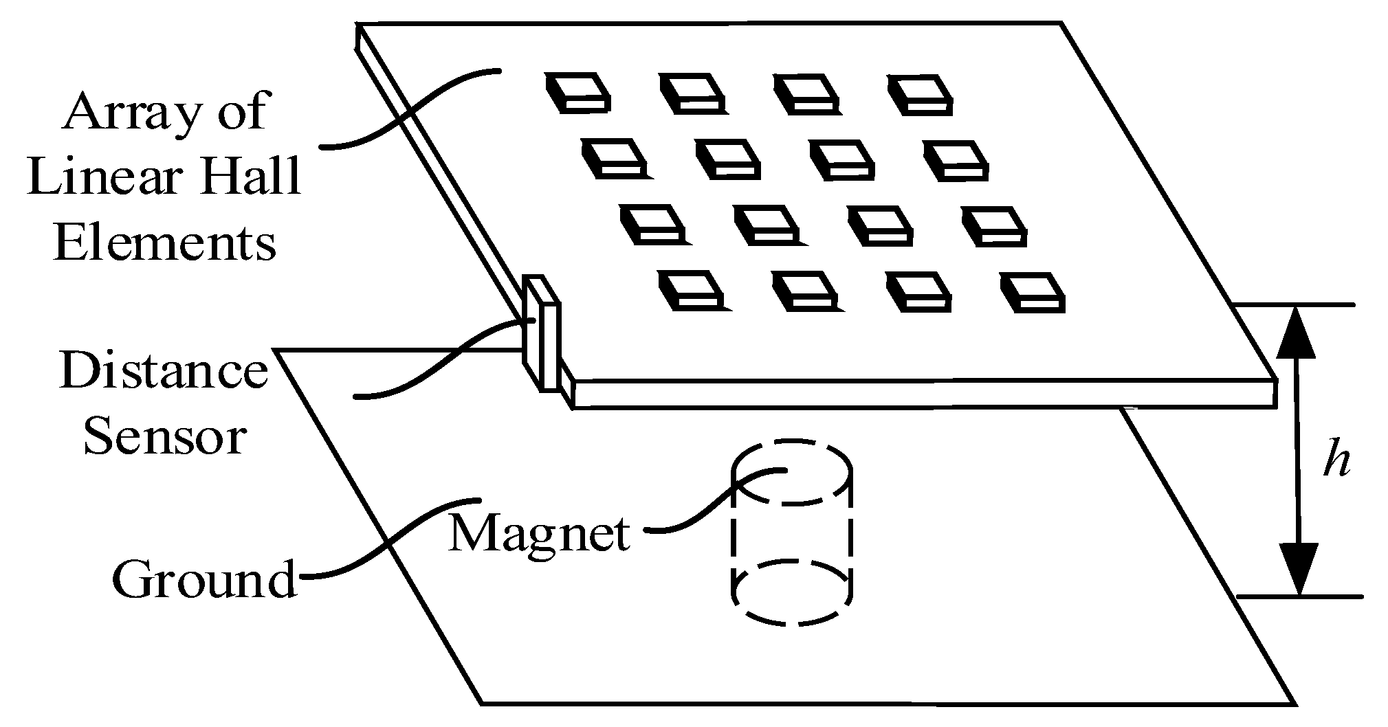
Due to the low accuracy of indoor positioning used in agricultural production, to ensure the accurate positioning of the agricultural robot, the magnet is installed on the ground, and the magnetic field strength of the ground magnet is acquired using the array of linear Hall elements on the agricultural mobile robot. Then the magnetic field strength is matched by using the acquired magnetic field data, and the combined device is shown in Figure 1.
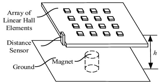
Figure 1.
Magnetic positioning device diagram.
As shown in Figure 1, a 4 × 4 array of linear Hall elements was installed on an agricultural mobile robot and a cylindrical permanent magnet was preburied under the concrete ground where precise positioning is required. The permanent magnets were placed in a regular grid and the grid spacing was 2 cm. Since the movement of the agricultural robot can change the distance between the array of linear Hall elements and the ground, the distance h between the linear Hall elements and the ground was obtained using a side-mounted distance sensor.
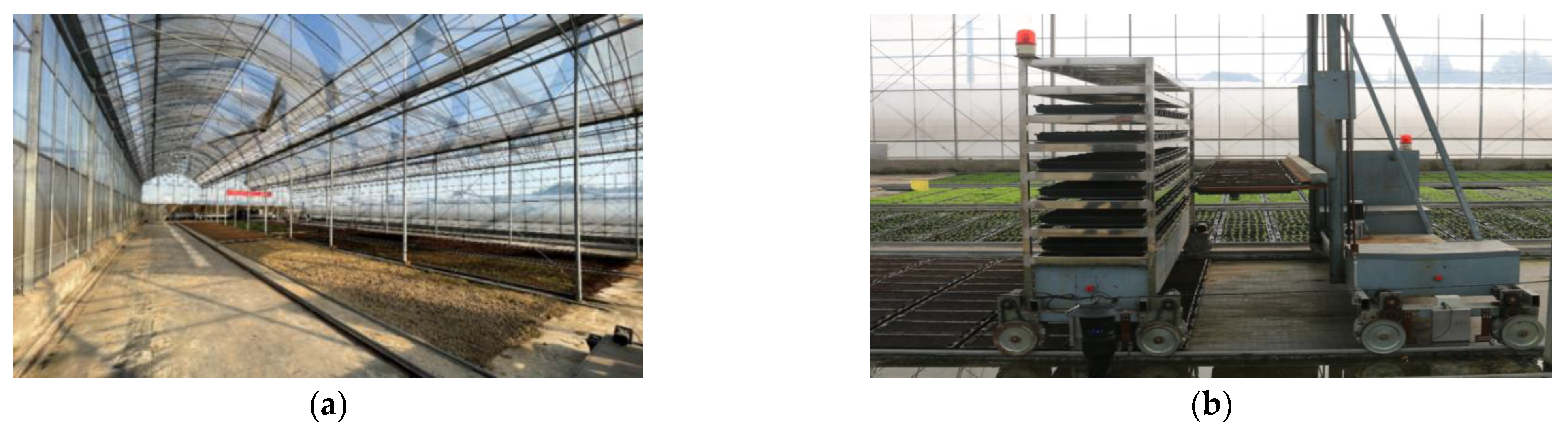
The magnet position was generally determined based on the magnetic force detection of the column magnet as a whole and the setting of the magnetic force threshold. Based on the aforementioned methods, this paper further analyzes the position determination based on the different magnetic force distributions of the cylindrical magnet from outside to inside, thus taking the positioning progress to the millimeter level. Since the agricultural mobile robot usually needs to install a separate computing unit with poor power, to ensure that the agricultural mobile robot could achieve accurate positioning, this paper first solved the analytical model of the magnetic field of the ground magnet and corrected the parameters in the model using finite element simulation values and field measurements. Then, it used the modified model for magnetic search, and optimized the search algorithm according to the magnetic field characteristics of the magnet, in order to finally achieve a positioning accuracy of the agricultural robot at key positions. The agricultural robot used in the experiment in this article is shown in Figure 2.
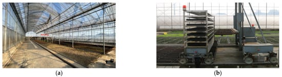
Figure 2.
The agricultural robot used in experiment. (a) The whole situation of facility factory nursery base. (b) 7Y-50 cavity tray intelligent transportation system.
2.2. The Selection of Sensor
The unmanned pendulum collection software system in this article matches the magnetic field by using the ground magnetic field collection data and the calculated magnetic field to achieve the accurate positioning of key locations. The magnetic field collection sensor needed to be selected to ensure the accuracy and stability of the data.
The linear induction Hall element of model SS495A1 was selected as the magnetic field sensing element for the ground magnetic field data collection of the vegetable base in this paper. The SS495A1 linear Hall sensor can convert the acquired magnetic field strength data into a voltage output and realize the conversion of analog to electric A/D. The magnetic flux range ±760 (Gauss) can be detected, the zero-point drift error was ±0.04%/°C, the sensitivity was 3.125 ± 0.094 mV/G, and the sensitivity drift error at room temperature was about 25°C is 0~0.06%/°C. The detailed parameters are shown in Table 2.
Table 2.
Permanent magnet parameter setting table.
In this paper, since the amount of data to be collected was large, and the data collected by the magnetic field needs to ensure a relatively uniform collection time, it was impossible to use the CD4051 in the infrared distance sensor acquisition module. Therefore, an external 16 channel voltage analog acquisition module based on the Modbus communication protocol was adopted. The working voltage of the module was 24 V DC voltage, and the data acquisition module was protected by overcurrent voltage. The module could realize data communication of 16 analog signals by Modbus protocol and data transmission by RS485. The data voltage range was 0–10 V, and the communication rate was 20 Hz. The collected data had 12-bit ADC accuracy, which could meet the data acquisition with a high baud rate without considering errors.
3. Analytical Solution Modeling of the Magnetic Field Strength of Permanent Magnets
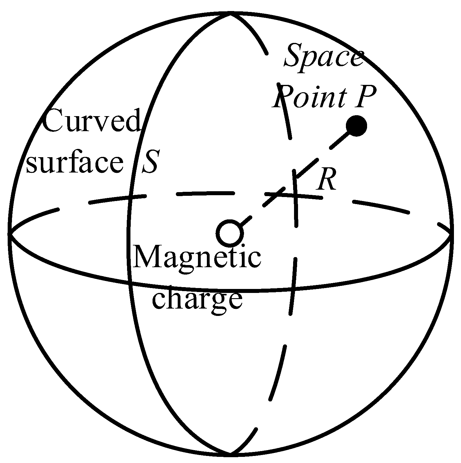
In the calculation of the spatial magnetic field of ground permanent magnets, the methods were generally the scalar magnetic potential method and the vector magnetic potential method. The corresponding differential equations were established by using the equations of magnetic scalar potential or magnetic vector potential in Maxwell’s equations, which could realize the numerical analytical calculation of the magnetic field, as shown in Figure 3. Since the Hall element used in this article only had the applied magnetic field strength when it was close to the magnet, the influence of the earth’s magnetic field and other artificial magnetic fields were negligible. Therefore, they were not considered in the modeling process of this article.

Figure 3.
Magnetic calculation model.
Using the equation for calculating the magnetic field of the magnetic charge model, the equation for calculating the magnetic scalar at any point P in the space near the permanent magnet [24] can be obtained as:
where M is the magnetization intensity of the cylindrical permanent magnet; S is the space surface outside the cylindrical permanent magnet; R is the distance between the magnetic charge and the space point, and n is the normal unit vector outside the magnet located on the magnet surface. The schematic diagram is shown as follows in Figure 4.
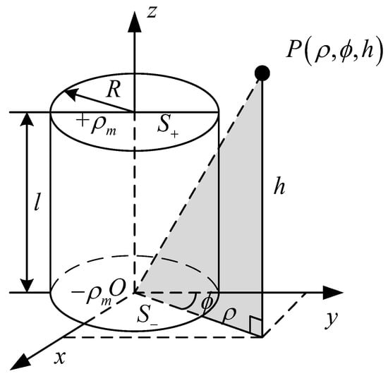
Figure 4.
Schematic diagram of cylindrical permanent magnet.
Define as the bound magnetic charge surface density, which represents the total directional vector value of the magnetic charge on the outer surface of the magnet:
Since it needed to be calculated as a magnetic field at any point in space, there was no need to calculate the magnetic charge inside the magnet, and only the magnetic charge on the top and bottom surfaces of the cylindrical permanent magnet existed. So, Equation (1) combined with Equation (2) can be simplified as follows:
According to the formula for the magnetic field strength in the magnetic charge equation, the magnetic field strength H at any point P in space can be obtained as:
where, is the divergence factor, which is used to indicate the strength of the vector divergence at each point in space within the characterization space, and the magnetic field strength H of the ground cylindrical permanent magnet can be calculated as:
The magnetic field distribution of the permanent magnet was obtained for Equation (5). The magnetic charge model was used in the analytical calculation, so the bound magnetic charge surface density is obtained as shown in Equation (6):
Substituting Equation (6) into Equation (5), the expression for the magnetic field from any point in space outside the cylindrical permanent magnet to the permanent magnet can be obtained as:
where is the angle between point P and the positive direction of the y-axis; is the distance between point P and the centerline of the permanent magnet; h is the distance between point P and the lower end face of the permanent magnet; i, j, and k are unit vectors in x, y, and z-axis directions respectively.
Equation (7) allows for the curved area partitioning of the magnetic charge surface. The magnetic charge surfaces and can be divided into ,,,,,. The magnetic field strength at a point can be found by calculating these six integrals respectively.
(1) Calculation of and
It is obtained that is:
Let , ≤ 1 satisfy the requirements of the generalized binomial theorem, and thus it follows that:
The integration region of Equation (9) is asymmetric and there is a nonintegrable issue in the process of binomial expansion, so a relative coordinate system is established at the projection point of point P on the -plane as in Figure 4, where the -axis of the -coordinate system is the line between point O and point . The projection of point P and the direction is the origin point O to the point . The -axis is at an angle of degrees from the x-axis and which is on -plane, and the -axis coincides with the z-axis, and the relative coordinate system as shown in Figure 5.

Figure 5.
Schematic diagram of relative coordinate system .
At this point, according to the established relative coordinate system, , it is obtained that:
Since in the binomial expansion is symmetric about the region of integration, it follows that in the direction of the unit vector there is:
(2) Calculation of and
According to the equation, eliminating the original equation and then defining the coordinate system, the binomial expansion of is obtained as:
where ,
Similarly, the binomial expansion of can be obtained as:
where ,.
It can be obtained that both and , which are based on the coordinate system. In order to establish the mapping relationship with the original xyz coordinate system, the magnetic field force needs to be decomposed, and according to the schematic diagram of the coordinate system as in Figure 4, it can be obtained that:
(2) Calculation of and .
Similarly, it is obtained that:
where ,
where ,
Substituting Equations (11) and (14)–(16) into Equation (7), it is obtained that:
By calculating the magnetic field strength above, the total magnetic induction of the cylindrical permanent magnet in the vacuum case (), can be calculated as:
where is the magnetic permeability of the space magnetic medium of the cylindrical permanent magnet.
4. Simulation of the Magnetic Field Strength of Permanent Magnets and the Magnetic Field Strength Formula Correction
4.1. Simulation of Magnetic Field Strength of Permanent Magnets
To ensure the accuracy of the magnetic field calculation for this equation magnet, ANSYS Maxwell magnetic field analysis software was used to simulate the cylindrical permanent magnet and compare the analytical calculated values with the finite element simulation values. The simulation process mainly defined material parameters, established a magnetic field model, set spatial domain boundary conditions, simulated results, and analyzed the cloud image.
(1) Define material parameters.
In this paper, the test used powerful magnets with magnet type NdFe35, and the specific parameter settings are shown in Table 3.
Table 3.
Permanent magnet parameter setting table.
(2) Modeling the magnetic field.
A cylindrical permanent magnet with a 5 mm upper face radius and a 20 mm magnet height was used for the test, as shown in Figure 6. The upper face of the permanent magnet is the N-pole of the magnet, and the lower face is the S-pole, and the magnet was placed vertically. We created a Maxwell 3D model in ANSYS Maxwell, set the individual cylindrical permanent magnet size parameters, and defined the material parameters.
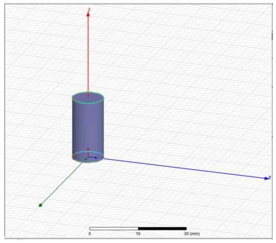
Figure 6.
Modeling of a single cylindrical magnet.
(3) Set the space field boundary conditions.
The magnetic field strength of the ground permanent magnet at different heights was measured using a digital Tesla meter. According to the field measurement, the digital Tesla meter was placed vertically with the ground permanent magnet position at 10 mm to 15 mm above. The magnetic field value at this position was measured, and the maximum value of the magnet magnetic field at 10 mm was about 0.65 T. Magnetic field strength range and indexing values that can be detected by the linear Hall sensor SS495A1 were set to the distance of the linear Hall sensor from the ground at about 15 mm in this simulation. According to this value, the finite element space domain was set as a square with a side length of 40 mm and set the parallel symmetry plane of the space domain.
(4) Result simulation and cloud image analysis.
A relative coordinate system located 15 mm from the upper-end face of the permanent magnet was established, and the xOy-plane of this coordinate system was used to calculate the magnetic field strength B and the simulation results were compared numerically. The simulation results in ANSYS Maxwell are shown in Figure 7.
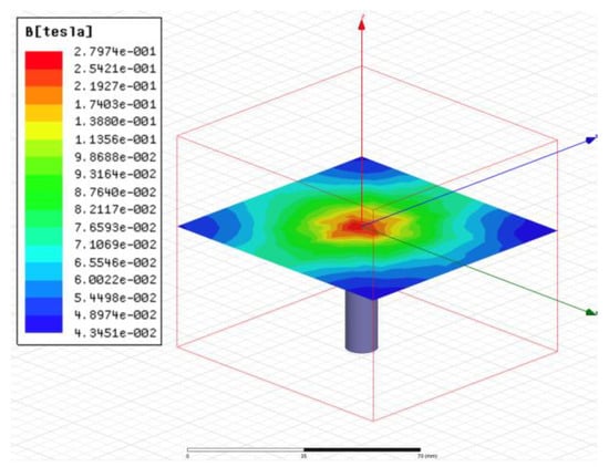
Figure 7.
Cloud image of magnetic field intensity.
4.2. Magnetic Field Strength Formula Correction
Two height positions of 10 mm and 15 mm were selected for the multipoint measurement of the magnetic field strength in the plane, and the data were filtered in these two planes in the ANSYS Maxwell dataset. Since the magnetic field of a single cylindrical permanent magnet was symmetrically distributed, so the distance was only used as the horizontal coordinate, and the comparison results are shown in Figure 8.
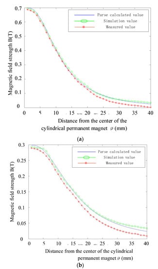
Figure 8.
Comparison of the calculated value, simulated value, and measured value. (a) Magnetic field 10 mm away from the upper-end face. (b) Magnetic field 15 mm away from the upper-end face.
As shown in Figure 8, the red star-shaped line is the real measurement value, the green circle-shaped line is the Maxwell magnetic field simulation value, and the blue line is the analytical calculation value. According to the calculation, the average error between the analyzed and measured values of magnetic induction strength B was 12.4%, and the average error between analyzed and simulated value was 6.63%. According to Equation (6), it is known that the analytical calculation only considers the upper and lower surfaces, so there was a numerical fluctuation between the analytical value and the simulated value at the edge of the upper-end face. Meanwhile, this paper considers the offset of the image caused by the deviation of computer calculation and data processing. The error between the analytical value and the field measured value increases with the increase of distance, and the value of multiple measurements was smaller than the calculated value, mainly considering that the magnet parameters have a certain error with the nominal, and the deviation at this place was larger. Therefore, the correction of Equation (18) was needed.
In order to realize the correction of the perturbation error of the magnetic field, the correction function that changed with the measurement position was added in the cylindrical permanent magnet analysis, and the correction function needed to consider the numerical correction of the magnetic field components in each direction in the relative coordinate system , and the correction function can be obtained as:
where is the coefficient of magnetic field distance correction.
Combining the relevant terms of Equations (18) and (19), the analytical calculation expression of magnetic field strength B is:
For the overall deviation of the data, add the magnetic field correction factor to Equation (20), can be calculated as follows:
where is the magnetic field deviation correction factor and is a correction function that varies with distance.
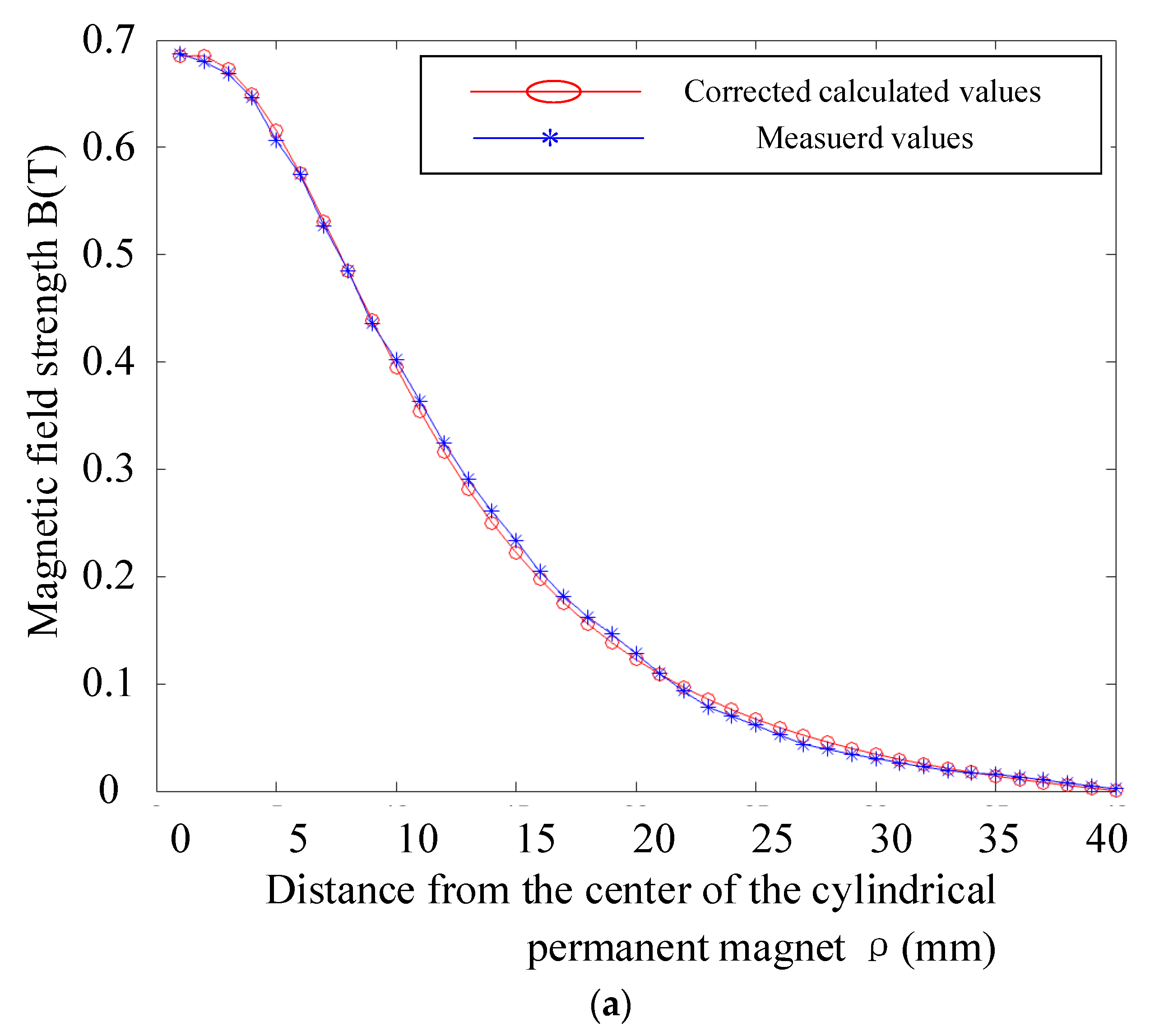
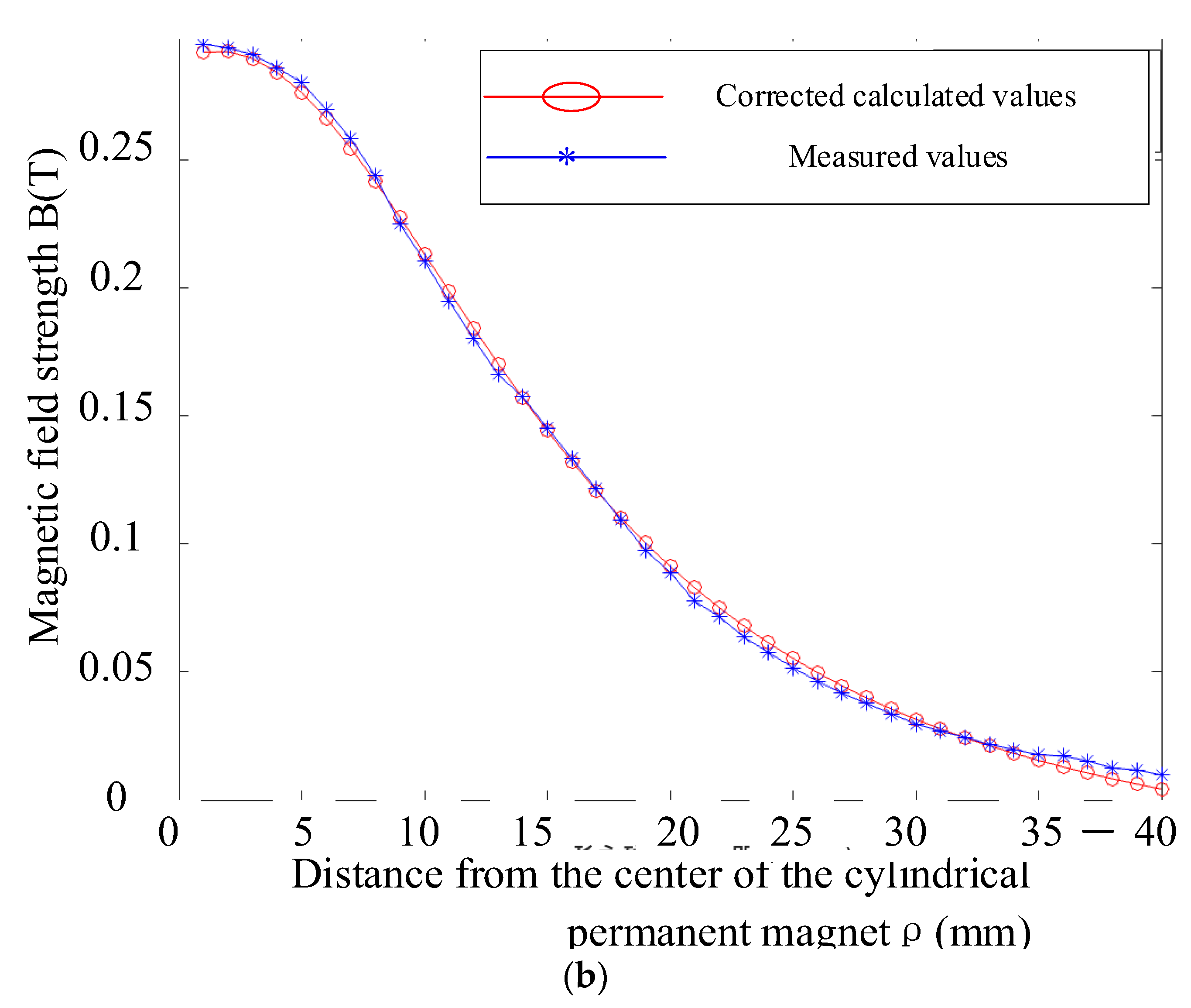
The parameters in Equation (21) were numerically fitted based on the measured values of the magnetic field strength and the analytical calculation results of the cylindrical permanent magnet at the cavity disk base. It is obtained that , , with a mean square error (MSE) of and an R-square of 0.999, compared as shown in Figure 9.
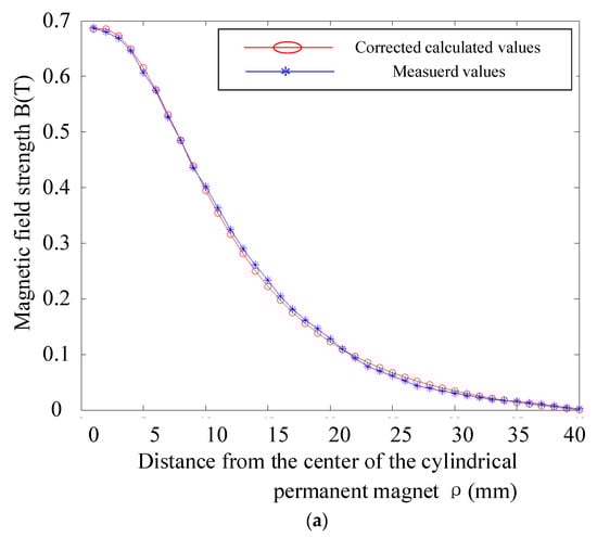

Figure 9.
Comparison between calculated and measured values after modification. (a) Magnetic field 10 mm away from the upper-end face. (b) Magnetic field 15 mm away from the upper-end face.
By calculating the magnetic field data at different distances from the end face and comparing it with the real measurement values, the results of the error rate are shown in Table 4. The corrected average error value is 6.61%, and the modified magnetic field analytical formula is within the error acceptance range.
Table 4.
Modified calculation error rate table for different distances.
5. Matching Model based on Magnetic Field Analytical Solution
5.1. Magnetic Field Matching Model
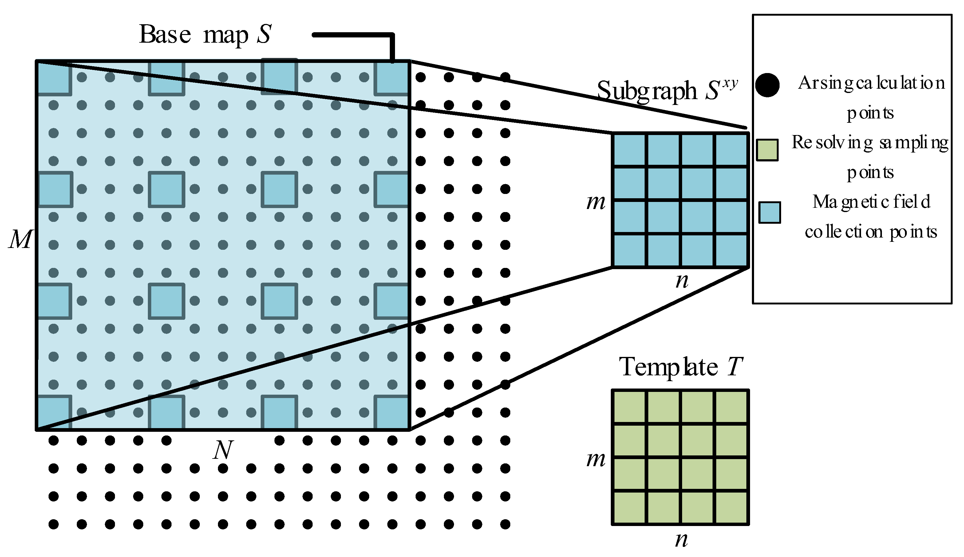
As the data density for the resolution calculation is 1 mm, the linear Hall elements are arranged at 5 mm intervals, so the density of the magnetic field detection array was much smaller than the calculated resolution density, and therefore the conventional grey-scale matching algorithm cannot match the data. The design of the magnetic field data with a base map S size of M × N, using a magnetic field template map T size of m×n, and a subgraph size of m×n, where (x, y) is the upper left corner of the subgraph in the base map S pixel coordinates, as shown in Figure 10.
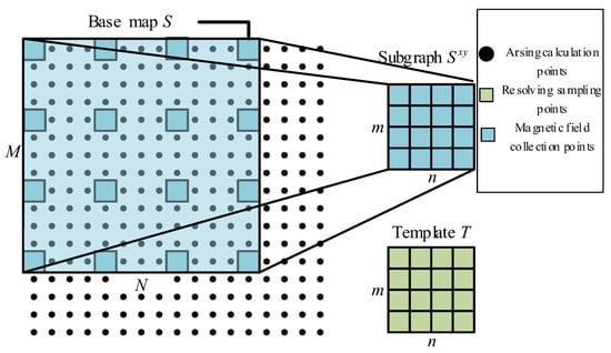
Figure 10.
Search graph, subgraph, and template graph.
Based on the subgraph established in Figure 10, a subgraph is constructed by sampling the search graph S at 5 mm intervals, which can be used to perform template matching with the template graph T.
In order to achieve comparison of the relevance of the template to the subgraph, the correlation function needs to be selected. The main common correlation functions are the MAD algorithm [25] and the SSDA algorithm [26], both of which have good template matching capabilities. These two algorithms are introduced as follow.
MAD algorithm.
The MAD algorithm is an algorithm used for matching, the main idea of which is to obtain a graph of the same size in the search graph S and the template graph T to calculate the average error value between the two graphs. In this paper, the search graph S is sampled with the template graph T for equal density, so the range of subgraph sampling x, y can be obtained as:
In the actual sampling process, there may be a part of the corresponding value of the subgraph , which exceeds the search map S boundary, where the boundary for the magnetic field value is small and can be neglected, so the complementary zero is used for the data exceeding the search boundary. From this, the matching degree function can be obtained according to the graphical relationship as in Figure 9.
The metric function is the matching metric value after offsetting (x,y). When the value at (x,y) is the minimum value among all the offsets, the best matching position is considered to be obtained after offsetting (x,y). In this paper, this position was considered as the accurate positioning position of the ground magnetic field and the measured magnetic field. At the same time, this algorithm has a strong antinoise ability and has a high matching accuracy when the distortion of the value changes is relatively small.
SSDA algorithm
The SSDA algorithm, also known as the sequential similarity detection algorithm, is an optimization of the MAD algorithm, which computes the mean values of the subgraphs and templates to obtain that:
According to Equations (24) and (25), the absolute error in template matching can be calculated as:
The constant error threshold was taken in the algorithm , the pixel point was randomly selected in the subgraph , and the absolute error value in the template graph T corresponding to it was carried out by Equation (26), and the error value was cumulated. When the total error value exceeded the error threshold after t times of cumulation, the cumulative number t at the point was recorded, so the relevant number t was defined with the cumulative value of the search at the location of the matching search graph as
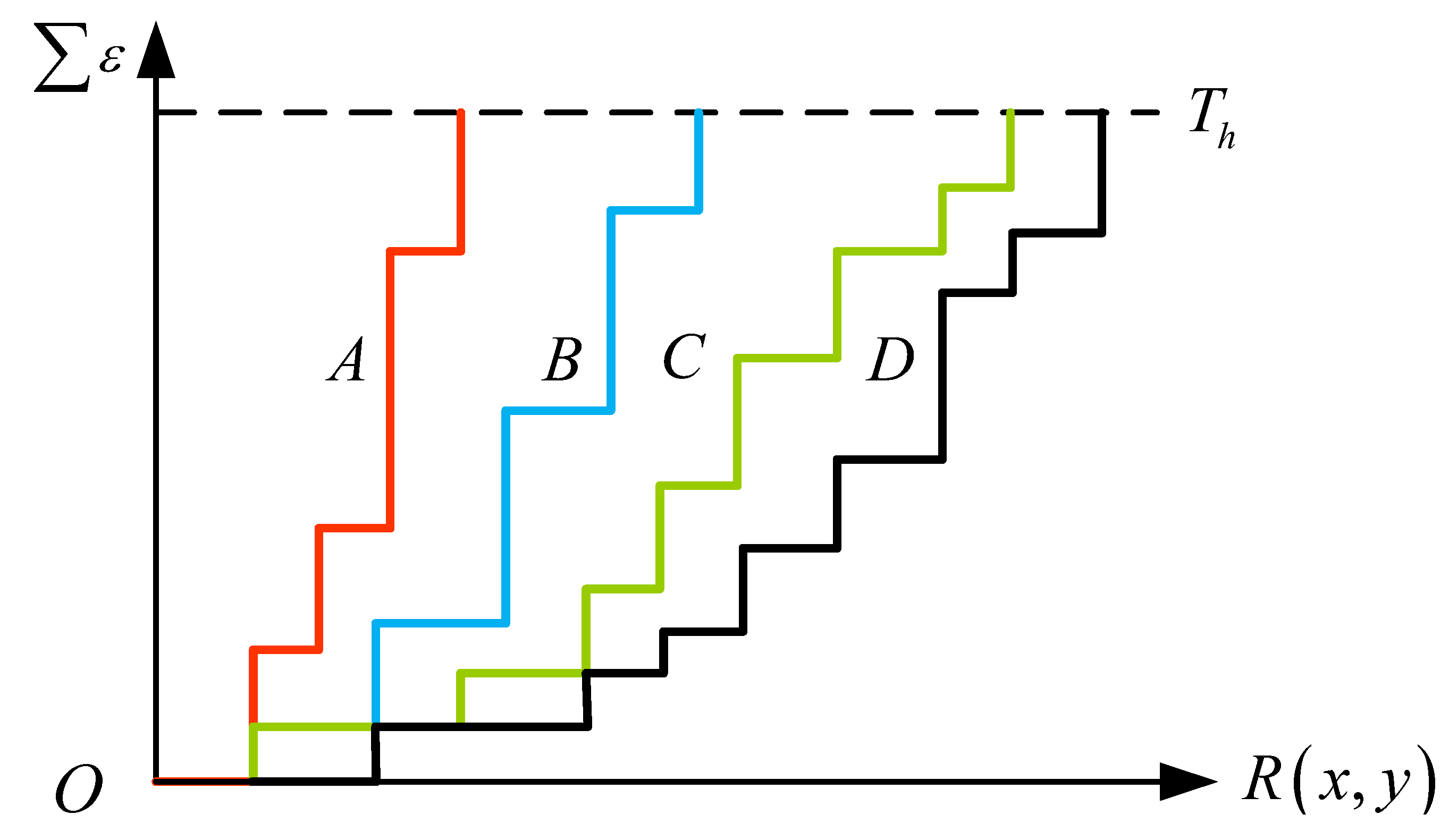
When was the maximum value in the search map, it was considered that the location at point was the matching position. Compared with the conventional MAD algorithm, the SSDA algorithm was able to select pixels by a nonrepetitive order, without calculating all pixels in the search map, as long as the total error value was greater than the set error threshold , it could quickly exclude subgraphs with large differences from the target template graph T, which could largely speed up the matching. However, due to the strong randomness of this method, if there was noise in the ground collection data, there may have been a situation where the matching t times were directly identified as a nontarget matching region, and the cumulative value of SSDA matching search for different subgraph is shown in Figure 11.
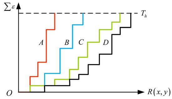
Figure 11.
SSDA algorithm matching chart.
As shown in Figure 11 above, when there was a large error between subgraph A and subgraph B and the collected value of the ground magnetic field, there existed a rapid growth of the accumulated absolute error. When the total accumulated error was greater than , the search for the submap was suspended. However, when there was more serious noise in submap C at the preset matching point, the matching result of the final SSDA algorithm was considered with submap D as the final matching position due to the larger error obtained from the calculation in the matching algorithm. Therefore, although the SSDA algorithm could quickly screen the nonmatching positions, it was less effective in matching the template T where noise exists.
The SSDA algorithm can be improved using the pyramid acceleration model, however, in this paper the actual ground magnetic field data collection points were relatively small, only pixels. Therefore, the pyramid acceleration algorithm showed a poor performance in up sampling and down sampling the images which needed to be matched, while the original SSDA algorithm can already be better applied in the magnetic field matching algorithm.
5.2. Magnetic Field Matching Model Optimization
In Section 4.2, both the search algorithm MAD and the random search algorithm SSDA required matching a global search. However, the global search will increase the computation of the main logic chip, so it requires optimization of the magnetic field matching model in Section 3. According to the problems existing in the above matching model, the model optimization was mainly reflected in the optimization of the analytical solution model of the cylindrical permanent magnet and the optimization of the search matching algorithm for the magnetic field acquisition data.
(1) Cylindrical permanent magnet model optimization
To ensure the accuracy of magnetic field matching, it was necessary to calculate the entire area of the ground cylindrical permanent magnet. However, as shown in Figure 8, when the magnetic field measurement point was located at 10 mm away from the upper end of the cylindrical permanent magnet while the distance from the projection position of the upper-end surface was more than 40 mm, the measured magnetic field strength value was less than 10 m. Although the value was still within the detectable range of the linear Hall element, when the distance exceeded 40 mm, the magnetic field value of the entire magnet changed slowly and the values converged to zero. Despite the fact that it did not affect subsequent calculations of the position of the magnetic field matching model, using Equation (21) numerical calculations of magnetic fields would increase numerical calculation time, reduce efficiency, and did not guarantee real-time magnetic field matching.
By setting the radius of the magnetic field influence, the amount of calculation of the analytical value of the magnetic field could be greatly reduced and the optimized magnetic field expression could be obtained as follows:
where for the magnetic field influence radius takes 40 mm.
(2) Search algorithm optimization
As the search graph obtained from the subgraph in this paper was the magnetic field value matrix of the ground cylindrical permanent magnet, the overall magnetic field data distribution was as shown in Figure 6. The value in Figure 6 is centered on the maximum magnetic field value of the magnet. All the data were symmetrical along the axis of rotation, and the overall data is slope shaped. Thus, the search algorithm could conduct a directional search according to the change direction of magnetic field data instead of using global search supplemented by a random search to achieve precise positioning of magnetic field matching. The magnetic field data trend is shown in Figure 12.
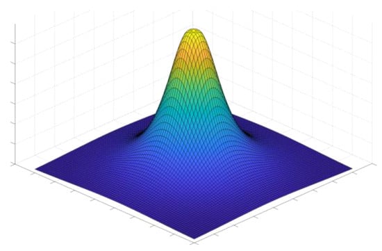
Figure 12.
Schematic diagram of surface magnetic field data trend.
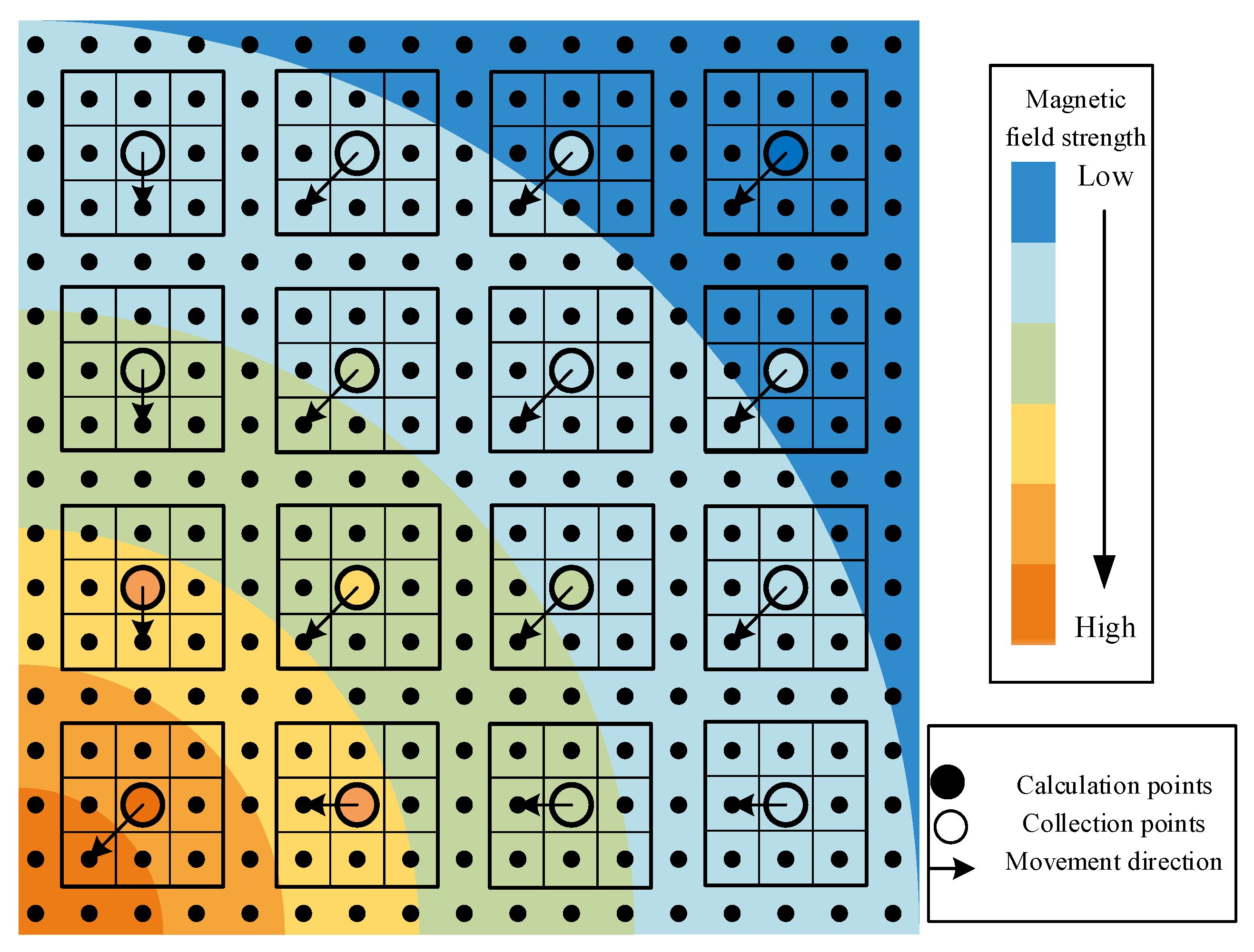
To achieve data movement, it was necessary to compare the ground data near the collection point with the collected value data, which is shown in Figure 13.
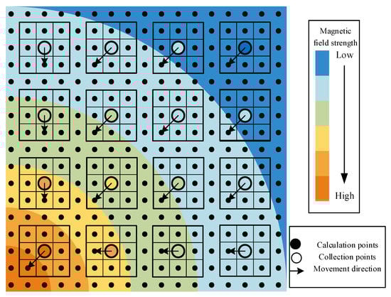
Figure 13.
Magnetic cloud map and data collection point schematic diagram.
According to the relationship between the ground collection point and the calculation point in Figure 13, the data in this paper were compared using eight numerical calculation points of the ground magnetic field near the collection point, located in the vicinity of the subgraph sampling point for the -direction calculation value . The optimal direction can be obtained through the calculation formula as follows:
The calculated direction was the minimum value of the data difference between the ground data collection point and the p-direction of the subgraph sampling point . Since the ground magnetic field collection module used in this paper was a 4 × 4 linear Hall element, it was necessary to count the optimal direction at these 16 points. If eight directions had the same data difference, the point was defined as having no optimal movement direction, and the common movement direction obtained from these 16 points was derived according to the way of seeking the combined force as follows:
Then, using the common motion direction to compare with the eight fixed directions, select the direction of the next subgraph movement, get the new subgraph search coordinates, and calculate the error value between the subgraph and the template map T at this time. When the error no longer decreases, stop the search and the best position for magnetic field matching is at .
As the improved method in this paper used one pixel movement at a time, the determination of the initial position had a greater impact on the number of final movements. According to the data characteristics in Figure 13, the maximum value of the 16 data acquired in the ground magnetic field acquisition module could be assumed to be the positive center of the magnetic field, which reduced the occurrence of too many search steps caused by subgraph staring from an unknown initial position. The advantage and the disadvantage of the algorithms mentioned above is shown in the Table 5.
Table 5.
The advantage and the disadvantage of the three algorithms.
5.3. Accurate Positioning Model Based on Magnetic Field Matching
Magnetic field matching of a single-sided ground cylindrical permanent magnet was achieved in Section 3, however, this method could only achieve the positioning of the agricultural mobile robot and the central position of the array detection, as shown in Figure 14.
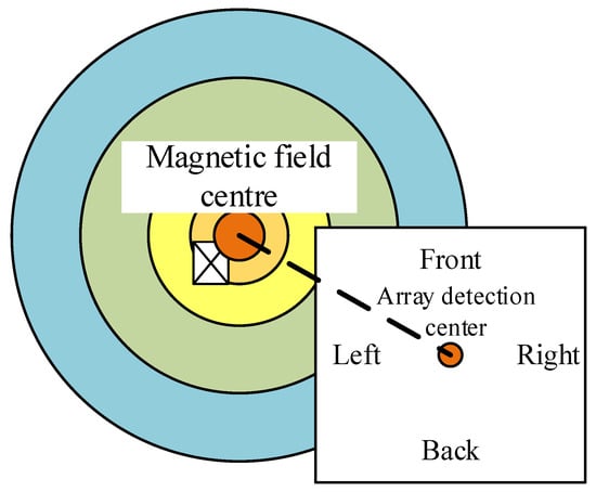
Figure 14.
Array linear Hall element location diagram.
As shown in Figure 14, the distance between the magnetic field center and the array detection center could be achieved by using the array linear Hall element. According to the data acquisition value of the array linear Hall element and the moving direction of the machine, the angular position relationship between the magnetic field center and the array detection center could be known.
Since the agricultural mobile robot may have a certain body angle deviation error during operation, it was impossible to correct the entire body angle only by using a single side magnetic field matching model. So, it was necessary to establish an accurate positioning method based on the magnetic field matching model.
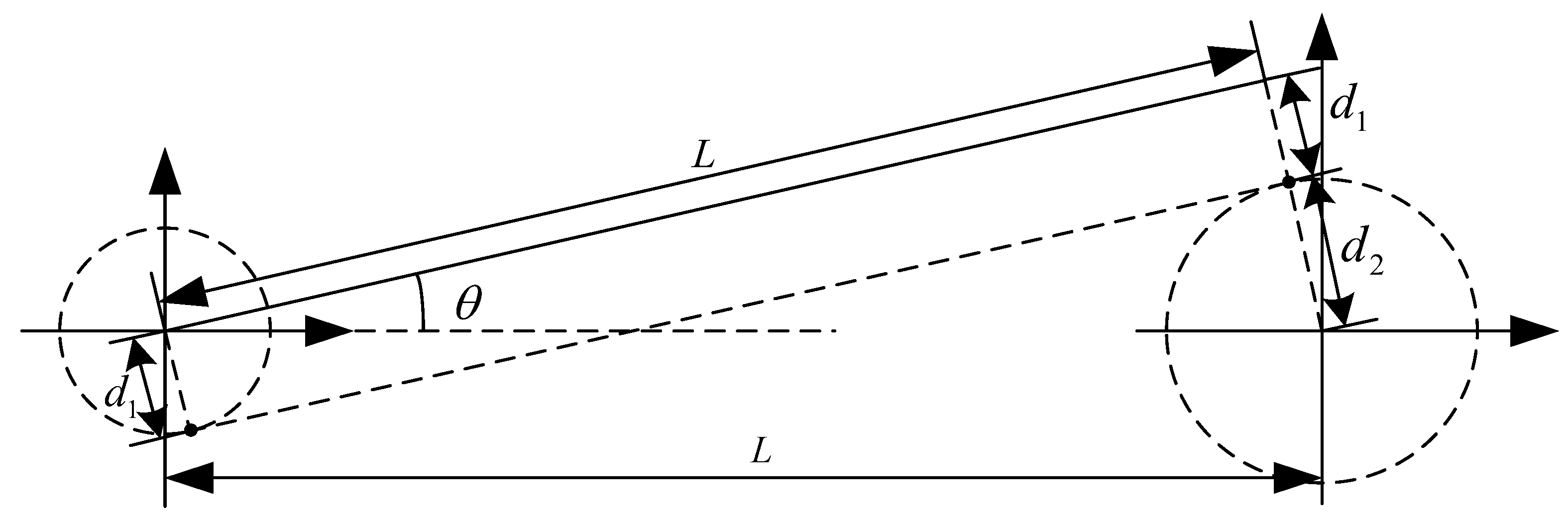
To implement this accurate positioning algorithm, a magnetic field matching model needed to be performed on both sides of the robot to obtain two offset data, which were divided into and , which are directional, as shown in Figure 15.
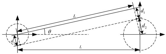
Figure 15.
Relationship between offset and Angle of machine.
As shown in Figure 15, the magnetic field matching results were and , respectively, and the interval between two magnetic field detection units was L. The results and , which were obtained in Section 4.2, were located on the left and right sides of the agricultural mobile robot. Meanwhile, depending on the angular position relationship between the magnetic field center and the array detection center as shown in Figure 14, the symmetric solution as shown in Figure 15 could be excluded. The one whole offset angle was based on the difference between this line segment and the angle between the parallel positions. The offset angle between the agricultural mobile robot and the parallel positions at this time can be calculated as:
Using the magnetic field-based matching model and Equation (31), the maximum angular error about the positioning error can be calculated as:
6. Accurate Positioning Result Analysis
The magnetic positioning device diagram and the setups can be tracked in Figure 1. The linear Hall element in the data acquisition module was used to collect the magnetic field value of the cylindrical permanent magnet at different positions, separately performed data acquisition, and determined acquisition location for multiple randomly selected locations. The hardware platform parameters used are shown in Table 6.
Table 6.
Software test hardware platform parameter table.
On the hardware platform, as shown in Table 5, the matching accuracy and the time spent on the matching algorithm were counted by using the MAD algorithm, the SSDA algorithm, and the improved search algorithm, respectively. The results are in Table 7. Among them, the MAD was used to calculate the error between the search graph and the template graph, through the scan of the whole search graph, and finally the accurate positioning position could be obtained. The SSDA was similar to the MAD, however, when the calculation error exceeded a certain threshold, the calculation process would be stopped and the next position would be matched. The improved search algorithm was based on the characteristics of the magnetic field changes of the cylindrical permanent magnet, using a similar way to gradient descent. It showed a strong relationship with low position error and short calculated time.
Table 7.
Magnetic field matching results.
As the driving speed was related to the magnet arrangement density, the key position error of the agricultural robot designed in this paper needed to be within 2 mm. The normal plane driving speed was designed to be about 0.3 m/s, which needed to be reduced to 0.05 m/s when approaching the key position, and the speed was adjusted to change the distance between the robot’s location and the key target position according to the environmental conditions of the facility. From Table 6, the original MAD algorithm had the best average error (0.365) in the ground magnetic field search with noise, however, the optimal value could only be obtained after completing a global search, so the running time was the longest (105 ms). Based on the MAD algorithm, the SSDA algorithm restricted a single subgraph search to a large extent. By setting the threshold value, the SSDA algorithm could quickly eliminate the position of unmatched subgraphs. However, due to the randomness of its threshold setting and the great impact on noise, the average running time of this algorithm was nearly seven times faster than that of MAD algorithm. The average error value of the SSDA algorithm was 2.671 mm, which did not meet the requirements of this paper for accurate positioning. The improved search algorithm based on the ground magnetic field in this paper could quickly move to the target position by searching down from the peak value of the magnetic field. The average error of this method was larger than that of the conventional MAD algorithm, however, the average error was within 1 mm, meeting the system design requirements, and the running time was nearly 50 times higher than that of the conventional MAD algorithm.
The agricultural mobile robot used in the experiment applied an improved search algorithm to achieve accurate positioning technology, which could achieve a magnetic field positioning error with an average error of 1 mm in a calculation time of 2 ms and could be offset by the Equation (31) computer body, and the value in Equation (28) was 40 mm. According to both sides of the array magnetic field detection device, it achieved the positioning distance error of ± 1 mm at the key position, the body angle error of ±0.02°, and met the unmanned harvesting system of facility vegetables cavity plate positioning accuracy requirements.
7. Conclusions
In this paper, the analytical model of the magnetic field of the cylindrical permanent magnet, which was embedded on the ground at the key position of the agricultural mobile robot was derived, and the results of the theoretical derivation were verified by combining the finite element simulation and the field measurement. In order to reduce the error between the analytical solution of the magnetic field and the field measurement value, the analytical model of the magnetic field was modified. Then, the magnetic field value of the ground cylindrical permanent magnet collected by the array linear Hall element magnetic field detection device was used and the position relationship model between the ground cylindrical permanent magnet center and the array magnetic field detection center was established using the magnetic field matching search algorithm. The array magnetic field detection device on both sides of the agricultural mobile robot was used to achieve the precise positioning function of key positions, with a positioning error of ± 1 mm, which meets the positioning accuracy requirements of the agricultural mobile robot. The contribution of this research can be summarized as below.
First, by improving the search algorithm (see Section 3 and Section 4), the position analysis on the magnetic force was conducted, and a high-precision and low-cost facility location method was obtained (compared with the existing infrared, ultrasonic, Bluetooth, and some other positioning technologies).
Regarding cost, this study mainly used the planned path to bury the cylindrical magnets and carried out the landfill according to a certain gap and density. By running in a straight line, lying sparsely, and being arranged densely at key positions, the consumption of magnets was reduced, and the costs could be reduced.
Regarding accuracy and time, compared with the MAD and SSDA, the improved search algorithm was more advanced both in position accuracy and time calculation. As shown in Table 4, the computational efficiency was improved by at least eight times.
In addition, this study can cooperate with the high-precision actuator on the moving platform, such as an intelligent picking robot and transplanting manipulator, etc., which can assist the actuator.
Author Contributions
Conceptualization, S.M.; Data curation, Y.S., Z.S. and F.P.; Format analysis, S.M.; Investigation, Y.S. and Z.S.; Methodology, S.M.; Validation, Z.S. and F.P.; Writing—original draft, S.M.; Writing—review & editing, Y.T. All authors have read and agreed to the published version of the manuscript.
Funding
This work is supported by the Jiangsu Agriculture Science and Technology Innovation Fund (JASTIF, CX (22)3100), Ningxia Hui Autonomous Region Science and Technology Program (2021BEF02001), Jiangsu Science and Technology Program (BE2018375), The Fruit, Vegetable and Tea Harvesting Machinery Innovation Project of Chinese Academy of Agricultural Sciences, and the National Key Research and Development Program of China (2016YFD0701503), the basic scientific research fund of research institute (S202103-01).
Institutional Review Board Statement
Not applicable.
Informed Consent Statement
Not applicable.
Data Availability Statement
Not applicable.
Conflicts of Interest
The authors declare no conflict of interest.
References
- Pei, F.Q.; Yang, K.W.; Wang, M.; Tong, Y.F. Analysis of application status of intelligent manufacturing in agricultural machinery. J. Intell. Agric. Mech. 2022, 3, 7–19. [Google Scholar]
- Liu, Q.; Zhu, Q.Y.; Feng, S. Review of indoor positioning technology. Computer Era. 2016, 8, 13–15. [Google Scholar] [CrossRef]
- Han, W.; Hao, L.; Cheng, H.L. Overview of indoor location technology. Smart Partn. 2018, 2, 133. [Google Scholar]
- Wang, X.X.; Cong, S. Review of indoor positioning research methods. Softw. Guide 2019, 18, 9–12. [Google Scholar] [CrossRef]
- Yao, W.Y.; Wei, L.X.; Zhang, H. Indoor Positioning design based on infrared beacon. J. Xuchang Univ. 2018, 37, 62–67. [Google Scholar]
- Li, J.K.; Feng, J.; Chen, J.Q. A Design of Ultrasonic Indoor Positioning System Based on Time Synchronized Wireless Network. Modern Radar. 2022, 44, 76–80. [Google Scholar] [CrossRef]
- Bu, X.Y.; Xiang, Y. Positioning Technology of intelligent mobile Robot. Sci. Technol. 2016, 26, 181. [Google Scholar] [CrossRef]
- Yang, H.J.; Hou, Y.Q.; Wang, L.X.; Cao, Y.L.; Jiao, H.T.; Yang, H. A ROS-based Bluetooth location-based courier delivery robot design. Technol. Innov. Appl. 2021, 11, 65–69, 72. [Google Scholar]
- Deng, K.D.; Qiang, S.; Ding, B.Y. Design of Concrete Unmanned Transportation Fleet Model System Based on Arduino and UWB Positioning Technology. Tech. Autom. Appl. 2020, 39, 143–145, 149. [Google Scholar]
- Zhao, S.W.; Ma, S.C.; Wu, S.M. Research on infrared and ultrasonic positioning technology. Value Eng. 2014, 33, 187–188. [Google Scholar] [CrossRef]
- Wei, L.X. Design and Research of Indoor Positioning System Based on Infrared Beacon Technology; North China Electric Power University: Beijing, China, 2018. [Google Scholar]
- Wang, P.; Wang, Y.; Wang, X.; Liu, Y.; Zhang, J. An Intelligent Actuator of an Indoor Logistics System Based on Multi-Sensor Fusion. Actuators 2021, 10, 120. [Google Scholar] [CrossRef]
- Song, Y.; Yu, W.J.; Cheng, C. Research on Indoor Geomagnetic Positioning Based on FCM Clustering and Location Area Switching. Mod. Electron. Technique. 2018, 41, 96–100. [Google Scholar]
- Liu, T.H. Indoor Positioning Using Magnetic Fingerprint Map Captured by Magnetic Sensor Array. Sensors 2021, 21, 5707. [Google Scholar]
- Jiang, S.C.; Liu, J.X. An Indoor Geomagnetic Positioning System Based on Smartphone. GNSS World of China. 2018, 43, 9–16. [Google Scholar]
- Zhang, C.C.; Wang, X.Y.; Dong, Y.N. Simultaneous Localization and Mapping Based on Indoor Magnetic Anomalies. Chin. J. Sci. Instrum. 2015, 36, 181–186. [Google Scholar]
- Sun, Z.S.; Wang, Q.; Luo, H.Y.; Tang, H.Y. Online Magnetic Fingerprints Based Personal Dead Reckoning Calibration Algorithm. Electron. Meas. Technol. 2017, 40, 147–152. [Google Scholar]
- Hou, X.L.; Xiu, B.G.; Zhou, Y.; Wang, D.S.; Lu, Y.J. Continuous Positioning Based on Multi-Sensor Fusion of GPS/INS/Magnetometer. Chin. J. Sens. Actuators 2020, 33, 1320–1326. [Google Scholar]
- Yu, Z.T.; Lv, J.W.; Zhang, B.T. A Method to Localize Magnetic Target Based on A Seabed Array of Magnetometer. J. Wuhan Univ. Technol. 2012, 34, 131–135. [Google Scholar]
- Hou, W.S.; Zheng, X.L.; Peng, C.L.; Wu, X.D. Study of Micro Medical Device Location System Inside Human Body Based on Permanent Magnet Field Detecting. Beijing Biomed. Eng. 2004, 2, 81–83, 87. [Google Scholar]
- Zhang, Y. Research on Magnetic Localization Technologies for Intelligent Vehicle. Shanghai Jiao Tong University, Shanghai. 2008. Available online: https://kns.cnki.net/kcms/detail/detail.aspx?dbcode=CMFD&dbname=CMFD2008&filename=2008052847.nh&uniplatform=NZKPT&v=bjpuOFfCRbxtD5yBZ-e-NMnVOmuHPcCiGlStfitNzBaOgkP2iV22AhRZWsuEhear (accessed on 1 December 2022).
- Wang, Z.; Song, T.; Wang, J.G.; Wang, Z.; Yang, C.Y. Differential Magnetic Localization Algorithm in High Background Magnetic Field and Its Application. Chin. J. Sci. Instrum. 2009, 30, 2384–2389. [Google Scholar]
- Li, G.; Sui, Y.T.; Liu, L.M. Magnetic Dipole Single-point Tensor Positioning Based on the Difference Method. J. Detect. Control 2012, 34, 5. [Google Scholar]
- Yi, J.Z. Magnetic Field Calculation and Magnetic Circuit Design; Chengdu Telecommunication Institute Press: Chengdu, China, 1987. [Google Scholar]
- Parra, L.; Spence, C. On-line convolutive blind source separation of non-stationary signals. J. VLSI Signal Process. Syst. Signal Image Video Technol. 2000, 26, 39–46. [Google Scholar] [CrossRef]
- Hashimoto, M.; Sumi, K.; Sakaue, Y. High-speed template matching algorithm using information of contour points. Syst. Comput. Jpn. 1992, 23, 78–87. [Google Scholar] [CrossRef]


Disclaimer/Publisher’s Note: The statements, opinions and data contained in all publications are solely those of the individual author(s) and contributor(s) and not of MDPI and/or the editor(s). MDPI and/or the editor(s) disclaim responsibility for any injury to people or property resulting from any ideas, methods, instructions or products referred to in the content. |
© 2022 by the authors. Licensee MDPI, Basel, Switzerland. This article is an open access article distributed under the terms and conditions of the Creative Commons Attribution (CC BY) license (https://creativecommons.org/licenses/by/4.0/).