Abstract
In this study, a nested ensemble filtering (NEF) approach is advanced for uncertainty parameter estimation and uncertainty quantification of a traffic noise model. As an extension of the ensemble Kalman filter (EnKF) and particle filter methods, the proposed NEF method improves upon the ensemble Kalman filter (EnKF) method by incorporating the sample importance resampling (SIR) procedures into the EnKF update process. The NEF method can avoid the overshooting problem (abnormal value (e.g., outside the predefined ranges, complex values) in parameter or state samples) existing in the EnKF update process. The proposed NEF method is applied to the traffic noise prediction on the Trans-Canada Highway in the City of Regina to demonstrate its applicability. The results indicate that: (a) when determining parameters in the traffic noise prediction model, the NEF method provides accurate estimation; (b) the model parameters can be recursively corrected with the NEF method whenever a new measurement becomes available; (c) the uncertainty in the traffic noise model (should be the noise itself) can be well reduced and quantified through the proposed NEF approach.
1. Introduction
Noise pollution continues to be a major health problem in the modern world, leading to various negative effects on human beings, such as cardiovascular effects, rising blood pressure, annoyance, sleep disorders, and learning impairment [1,2,3,4,5,6]. Noise is a major issue that should be considered during the design and construction of new transportation systems, as well as in the improvement of existing systems [7,8,9,10]. Road traffic noise is caused by the combination of rolling noise, consisting of friction noise between the road surface and the car tyres, and the propulsion noise caused by the exhaust systems or engines. The emission of traffic noise is influenced by many factors such as type of engines, exhaust systems and tyres interacting with the road, weather, and road conditions. For instance, Lictitra et al. [11] revealed the influence of tyres on the use of the Close Proximity Method (CPX) for evaluating the effectiveness of a noise mitigation action based on low-noise road surfaces. Further, some studies have been proposed to address the effects for pavement age, pavement texture, and other pavement characteristics on traffic noise emission [12,13,14,15,16]. Traffic noise prediction models are required as aids in the design of highways and other roads, and sometimes in the assessment of existing or envisaged changes in traffic noise conditions [17,18]. However, due to the complexities of urban traffic systems, extensive uncertainties exist in the traffic noise prediction model.
Previously, a number of uncertainty analysis methods have been applied to traffic noise prediction models. For example, Peng and Mayorga [19] assessed the impact of traffic noise based on probabilistic and fuzzy approaches under uncertainty, in which the input (i.e., traffic flow, speed, and component) of the traffic noise prediction model was represented by probability distributions. Gimenez and Gonzalez [20] introduced a stochastic model to describe and predict the noise levels, in which a Gaussian Ornstein–Uhlenbeck model is used to represent the dynamics of the noise levels, and the mean-reversion properties and seasonal volatility for each day of the week are studied separately. Ramirez and Dominguez [21] presented the development and evaluation of a stochastic dynamic traffic noise prediction model based on noise curves for vehicle classes and their speed. Iannone et al. [22] evaluated the influence of speed distribution in road traffic noise prediction. Huang et al., [23] used the entropy-copula method for modelling the dependence between traffic volume and traffic noise on the highway. However, previous studies of the uncertainty assessment in traffic noise predictions were mainly focused on inputs, such as the probabilistic characteristics of the road traffic flows [24]. Few studies have been conducted on the parameter estimation and uncertainty quantification of the traffic noise prediction models.
Therefore, in this study, a nested ensemble filtering (NEF) approach, as an extension of previous ensemble Kalman filter (EnKF) and particle filter methods, will be proposed for parameter estimation and the uncertainty quantification of traffic noise models. The proposed NEF method will improve upon the ensemble Kalman filter (EnKF) method by incorporating the sample importance resampling (SIR) procedures into the EnKF update process. Compared with the EnKF method, the proposed NEF approach can avoid the overshooting problem (abnormal value (e.g., outside the predefined ranges, complex values) in parameter or state samples) existing in the EnKF update process. The proposed NEF method will be applied to traffic noise prediction on the Trans-Canada Highway in the City of Regina to demonstrate its applicability.
2. Methodology
In recent decades, data assimilation methods have attracted increasing attention in various fields, such as traffic estimation, hydrologic forecasts, and so on. Sequential data assimilation is a general framework whereby system states and parameters are recursively estimated/corrected when new observations are available. In a sequential data assimilation process, the evolution of the simulated system states can be represented as follows:
where f is a nonlinear function expressing the system transition from time t-1 to t, in response to model input vectors ut and θ; is the analyzed (i.e., posteriori) estimation (after correction) of state variable x at time step t − 1; is the forecasted (i.e., priori) estimation of state variable x at time step t; θ represents time-invariant vectors, and is considered as process noise.
When new observations are available, the forecasted state can be corrected by assimilating the observations into the model, based on the output model responding to the state variables and parameters. The observation output model, in general form, can be written as:
where h is the nonlinear function producing forecasted observations and vt is the observation noise.
The essential methods for updating states is based on Bayesian analysis, in which the probability density function of the current state, given the observation, is approximated based on the recursive Bayesian law:
where represents the prior information, is the likelihood, and represents the normalizing constant. If the model is assumed to be Markovian, the prior distribution can be estimated via the Chapman–Kolmogorov equation:
Similarly, the normalizing constant can be obtained as follows:
The optimal Bayesian solution (i.e., Equations (3) and (4)) is difficult to determine since the evaluation of the integrals might be intractable [25].Consequently, approximate methods are applied to treat the above issues. The ensemble Kalman filter (EnKF) and particle filter (PF) are two of the most widely used methods. The central idea of EnKF and PF is to represent the state probability density function (pdf) as a set of random samples, and the difference between these two methods lies in the way of recursively generating an approximation to the state pdf [26].
2.1. Ensemble Kalman Filter
The ensemble Kalman filter (EnKF) is a Bayesian approach which aims to approximate the posterior distribution by a set of random samples. In the EnKF, the distributions are considered to be Gaussian, and the Monte Carlo approach is applied to approximate the error statistics, as well as to compute an approximate Kalman gain matrix for updating the model and state variables.
Consider a general stochastic dynamic model with the transition equations of the system state expressed as:
where xt is the sate vectors at time t; θ is the system parameters vector which are assumed to be known and time invariant; the superscript f indicates the “forecast” sates; the superscript a indicates the “analysis” states; ne represents the number of ensembles; ut is the input vector (deterministic forcing data); f represents the model structure; ωt is the model error term, which follows a Gaussian distribution with zero mean and covariance matrix . For the evolution of the parameters, it is assumed that the parameters follow a random walk, presented as:
Prior to the update of the model states and parameters, an observation equation is applied to transfer the states into the observation space, which can be characterized as:
where yt+1 is the observation vector at time t + 1; h is the measurement function relating the state variables to the measured variables; vk + 1,i reflects the measurement error, which is also assumed to be Gaussian with zero mean and covariance matix . The model and observation errors are assumed to be uncorrelated, i.e., . After the prediction is obtained, the posterior states and parameters are estimated with the Kalman update equations as follows [27]:
where yt is the observed values; represents the observation errors; Kxy and Kθy are the Kalman gains for states and parameters, respectively [28]:
Here Cxy is the cross covariance of the forecasted states and the forecasted output ; Cθy is the cross covariance of the parameter ensembles with the predicted observation ; Cyy is the variance of the predicted observation; Rt is the observation error variance at time t.
2.2. Particle Filter
Particle filters, similar to the EnKF, are sequential Monte Carlo methods that calculate the posterior distribution of states and parameters by a set of random samples. The advantage of the PF, in comparison to the EnKF, is that it relaxes the assumption of a Gaussian error structure, which allows the PF to more accurately predict the posterior distribution in the presence of skewed distributions [27,28]. In detail, consider ne independent and identically distributed random variables for i = 1, 2, …, ne, the posterior density, based on the sequential importance sampling (SIS) method, can be approximated as a discrete function:
where is the posterior (updated) normalized weight of the ith particle drawn from the proposed distribution and δ is the Dirac delta function. Assume the system state to be a Markov process, and apply the Bayesian recursive expression to the filtering problem. The updated expression for the importance weights (not normalized) can be expressed as:
Equation (14) provides the mechanism to sequentially update the importance weights, given an appropriate choice of the proposal distribution . Consequently, the expression of the proposal distribution will significantly affect the efficiency and complexity of the PF method. A common choice of the proposal distribution is the transition prior function [25]:
When the transition prior is chosen as the proposal distribution, Equation (14) can be simplified as:
Therefore, the normalized updating weight can then be obtained via the following equation:
where can be obtained from the posterior likelihood equation:
is the posterior likelihood function. If a Gaussian model error is to be used, the likelihood may be approximated via a parametric likelihood function:
For the particle filter through SIS, a serious limitation is the depletion of the particle set, which means that, after a few iterations (time steps), all the particles except one are discarded because their importance weights are insignificant [27]. To address the above issue, sampling importance resampling (SIR) algorithms are usually applied to eliminate the particles with small importance weights, and replace them with the particles with large importance weights. In our study, the sampling importance resampling (SIR) particle filter is implemented as elaborated by Moradkhani et al. [28], in which are set equal to 1/ne before moving on to the next time step, and the posterior weight is equal to .
2.3. The Nested Ensemble Filtering Approach for Parameter Estimation and Uncertainty Quantification
In the state and parameter estimation process through EnKF, one of the main problems is overshooting, which means that the parameters or states show abnormal values (e.g., negative, complex values) so that the data assimilation process cannot continue anymore, or wrong parameter and state values are generated. Therefore, to overcome this problem, a nested ensemble filtering (NEF) approach will be proposed, in which the SIR procedures will be integrated into the EnKF updating process to eliminate abnormal values [29,30]. The full description of the nested ensemble filtering processes is illustrated in Figure 1.
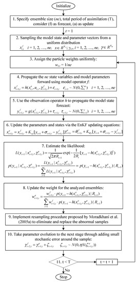
Figure 1.
The flow chart of the nested ensemble filtering method.
- Model state initialization: Initialize Nx-dimensional model state variables for ne samples: xt,i, i = 1, 2, …, ne, .
- Parameter sampling: Sample Nθ-dimensional model parameters for ne samples:θt,i, i = 1, 2, …, ne, .
- Sample weight assignment: Assign the particle weights uniformly:wt,i = 1/ne.
- Model state forecast step: Propagate the ne state variables and model parameters forward in time using model operator f
- Observation simulation: Use the observation operator h to propagate the model state forecast:
- Parameters and states updating: Update the parameters and states via the EnKF updating equations
- Estimate the likelihood:
- Obtain the updated weight for the analyzed ensemble values:
- Resampling: Apply the resampling procedure proposed by Moradkhani et al. [28] to eliminate the abnormal samples and replace the analyzed and .
- Parameter perturbation: Take parameter evolution to the next stage by adding small stochastic error around the sample:where η is a hyper-parameter which determines the radius around each sample being explored and is the standard deviation of the analyzed ensemble values.
- Check the stopping criterion: If measurement data are still available in the next stage, t = t + 1, return to Step 3. Otherwise, stop.
3. Applications
3.1. Statement of Problem
The City of Regina is the capital city of the Canadian province of Saskatchewan, located at 50°27′17″ N and 104°36′24″ W. It is the second largest city in the province, having a population of about 215,000. The City of Regina can be reached by several highways, including the Trans-Canada Highway from both the west and east sides and four provincial highways from other directions. The city is served by the Ring Road, a high speed connection between Regina’s east and northwest that loops around the city’s east side (the west side of the loop is formed by Lewvan Drive) with future plans to construct another perimeter highway to encircle the city farther out [31]. This type of highway with no traffic lights is one of the important sources of traffic noise, and typical to most Canadian cities.
To evaluate the performance of traffic noise modelling in different road aging conditions, three locations, namely A, B and C as shown in Figure 2, are selected as the measuring sites. As can be seen from Figure 2, these sites are distributed along the Trans-Canada Highway on which the speed limit is 100 km/h. More significantly, the sites are very close to each other with similar traffic and road construction conditions. Site A is a special site locate along Assiniboine Ave to Wascana Pkwy in the City. Before 4 October 2013, this way was an old pavement before it was repaved with a new pavement. Site B, from Wascana Pkwy to Assiniboine Ave, is paved with new pavement materials and selected for measuring the noise data and comparing to that of the old pavement under very similar conditions. Further, site C, from Albert St to Wascana Pkwy, was formerly old pavement before being paved in the summer of 2012, and experiments were conducted to find the noise effects of the old pavement. As shown in Figure 2, the surrounding environment and road construction conditions of these three sites are similar. There are no barriers or trees which will influence the sound propagation and thus affect the sound measurement, between the road and sound analyzer (as indicated in Figure 3).
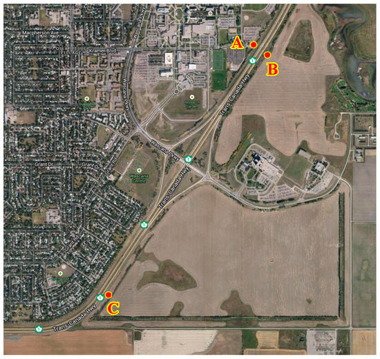
Figure 2.
Selection of the measuring sites.
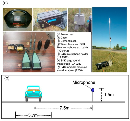
Figure 3.
Traffic noise measurement instrument (a) and installation (b).
The sound pressure levels for each selected site are measured by utilizing the B&K Modular Precision Sound Analyzer 2260 produced by Brüel & Kjær in Denmark, as shown in Figure 3a. Sound Analyzer 2260 supports one-channel measurements of environmental noise and noise at work, have a resolution/accuracy from 6.3 Hz to 20 kHz in 1/3-octaves of the frequency range. The setup of the experiments also refers to Bérengier’s research which considered the impact of traffic flow management on overall noise pressure levels [32]. The layout of the microphone adopted in the experiment is shown in Figure 3b, in which the microphone is placed 1.5 m above the ground and 7.5 m away from the center line of the highway.
3.2. Traffic Noise Emission Model
In noise studies, several different types of weighting network are performed on sound spectra to calculate the equivalent sound level for different objectives. Although there is criticism that A-weighting is not well correlated with the human perception of loudness [33], A-weighting is the standard weighting for outdoor community noise measurements and is commonly used for noise measurements within architectural spaces and vehicles [34]. Thus, in the present study, the equivalent traffic noise levels and the corresponding requirements are collected in the form of “A” weighted equivalent continuous sound levels (LAeq).
In addition, traffic noise from a stream of vehicles varies over time in strength depending on many different factors such as the number of vehicles that passed by, speeds of the vehicles, weather conditions in the tests, and so on. The time averaged noise level is employed to convert the fluctuating values of a certain time interval into a simple mean value. An important noise level indicator adopted by many standards to estimate the impact of long-term noise to humans, the continuous 24-h time-averaged noise level (LAeq 24h) is adopted as the long-term interval noise indicator. This is used for comparing the acoustic performances of new and old pavements in the present research. Tespite the fact that traffic flow conditions are different at all times, but over a period of 1-h, it may not fluctuate significantly. As a result, a 1-h time-averaged noise level (LAeq 1h) is another long-term noise indicator adopted in the research, as well as 24-h time averaged noise levels. In this study, the notion of “long-term” merely refers to the noise statistics (i.e., LAeq 24h, LAeq 1h) and does not indicate other factors (e.g., traffic flow).
Many studies have reported to address traffic noise prediction [35,36,37]. Some studies indicated that traffic noise intensity and traffic flow volume obey a logarithmic relation [38,39,40]. Consequently, an empirical traffic noise prediction model will be employed as follows:
where Q is the volumes of the traffic flow, while A and B are parameters relying on the pavement and test conditions and can be determined by experiments.
4. Results Analysis and Discussion
4.1. Parameter Estimation and Uncertainty Quantification of Traffic Noise Prediction Model at Scenario A1
Site A is a special site located along Assiniboine Ave to Wascana Pkwy in the City. Before 4 October 2013, this way was an old pavement, and then it was repaved. Consequently, the empirical traffic noise prediction model, expressed as Equation (20) was applied to Site A under both old and new pavement conditions. In this study, Site A with the old pavement conditions is denoted as scenario A1. Before the data assimilation process, initial ensembles would be sampled from predefined intervals. As presented in Table 1, the ensembles of A and B were uniformly sampled from predefined intervals. Figure 4a presents the generated traffic noise prediction function based on those initial samples. In Figure 4, the green lines are generated based on the initial and final ensemble values of A and B; the red stars indicate the actual measurements; the red line displays the curve of Model (20) with A and B estimated through the maximum likelihood estimation method. As can be seen from Figure 4a, large uncertainty exists in noise prediction.

Table 1.
Estimation results for the two parameters (A and B) in Model (20) under the four scenarios.
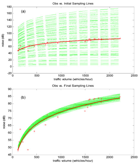
Figure 4.
Initial (a) and updated (b) traffic noise prediction curves in scenario A1.
Based on the noise measurement in scenario A1, the uncertainty in the traffic noise prediction model can be significantly reduced. As presented in Table 1, the mean values of the updated coefficients are closer to their corresponding values obtained through maximum likelihood estimation compared to the initial ones. Further, standard deviations of the updated coefficients are reduced dramatically throughout the data assimilation process, and thus the uncertainty of the coefficients has been greatly mitigated.
Figure 5 depicts the variations of coefficients A and B versus time. Significant uncertainty is found to be associated with the coefficients at the early stage of the assimilation process, though it is generally reduced as time proceeds. Eventually, the uncertainty of the traffic noise prediction model with the updated coefficients was significantly reduced, as shown in Figure 4b. Figure 6 presents a comparison between the forecasts of the traffic noise prediction model with updated coefficients and the actual measurements. This indicates that the predicted interval, with a confidence level of 0.1, can cover most measurements at Site A under old pavement conditions.
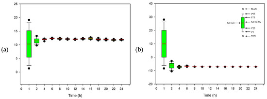
Figure 5.
Variations of parameters (a) and (b) in Model (20) during the data assimilation process under scenario A1.
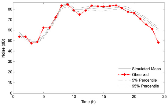
Figure 6.
Comparison between the predictions and observations in scenario A1.
In this study, the Pearson correlation coefficient (R2) is employed to compare the performance of the proposed nested ensemble filtering method and traditional maximum likelihood estimation method. Since the traffic noise prediction model still contains some uncertainty after the data assimilation process, leading to uncertain forecasts for noise emission levels, the mean values of these uncertain forecasts will be applied to calculate the R2 values. As can be seen in Table 2, both the NEF and MLE approaches can perform well in estimating the unknown parameter in Model (20) at Site A with old pavement.
Table 2.
Comparison of performance between the nested ensemble filter (NEF) and maximum likelihood estimation (MLE) methods.
4.2. Parameter Estimation and Uncertainty Quantification of Traffic Noise Prediction Model at Scenario A2
In scenario A2, measurements were still undertaken at Site A, as shown in Figure 2. The differences between scenario A1 and A2 is that the measurement was taken after 4 October 2013, when the road around Site A was repaved. Similar to the process in Scenario 1, initial ensembles would be sampled from predefined intervals (as presented in Table 1) for the model parameters, which leads to extensive uncertainties in model forecasts, as shown in Figure 7a. When measurements are available at Site A, the uncertainty in model parameters (i.e., A, B) would be reduced significantly (as shown in Figure 8). Consequently, the noise predictions by Model (20) can also be mitigated significantly, as can be seen in Figure 7b.
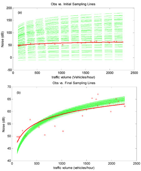
Figure 7.
Initial (a) and updated (b) traffic noise prediction curves in scenario A2.
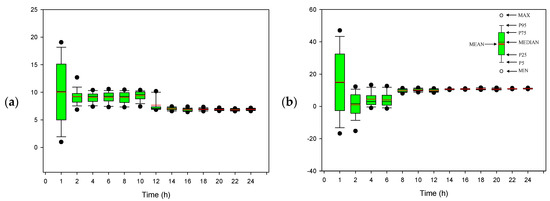
Figure 8.
Variations of parameters (a) and (b) in Model (20) during the data assimilation process under Scenarios A2.
As can be seen from Figure 8, significant uncertainties exist in the coefficients of Model (20) at the early state of the assimilation process. As more measurements are available, these uncertainties could be dramatically reduced, and eventually be compressed within very narrow intervals (i.e., [6.7, 7.2] for A and [10.5, 11.4] for B, as presented in Table 1). Figure 9 presents a comparison between the forecasts of the traffic noise prediction model with updated coefficients and the actual measurements. This indicates that the predicted intervals can generally reflect the fluctuation of the actual noise emission levels under new pavement condition.
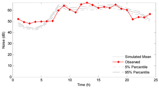
Figure 9.
Comparison between the predictions and observations in Scenario A2.
As presented in Table 1, the parameter values of A and B estimated by the nested ensemble filtering approach are quite different to those obtained through maximum likelihood estimation method. However, from the values in Table 2, we can find that the NEF method performed a little bit better than the MLE method, with the R2 values of NEF and MLE being 0.7649 and 0.7639, respectively.
4.3. Parameter Estimation and Uncertainty Quantification of Traffic Noise Prediction Model at Scenario B
Scenario B corresponds to Site B located on the road from Wascana Pkwy to Assiniboine Ave, as depicted in Figure 2. The road around Site B was just paved before our measurement, and was considered as new pavement condition. Figure 10 presents the initial and final results of Model (20). There is initially great uncertainty in Model (20), as indicated by the green lines in Figure 10a; such uncertainty would be effectively reduced after data assimilation by NEF (i.e., green lines in Figure 10b). During the data assimilation process, the uncertainties in parameters A and B in Model (20) are dramatically decreased, as shown in Figure 11. After the data assimilation process, the uncertainty of the traffic noise model can be quantified with the parameter values selected with the updated intervals (as stated in Table 1). Figure 12 shows the comparison between the predicted intervals and observations in scenario B. This suggests that the forecasts can generally reflect the actual variations in noise emission levels.

Figure 10.
Initial (a) and updated (b) traffic noise prediction curves in scenario B.
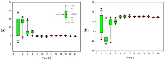
Figure 11.
Variations of parameters (a) and (b) in Model (20) during the data assimilation process under scenario B.
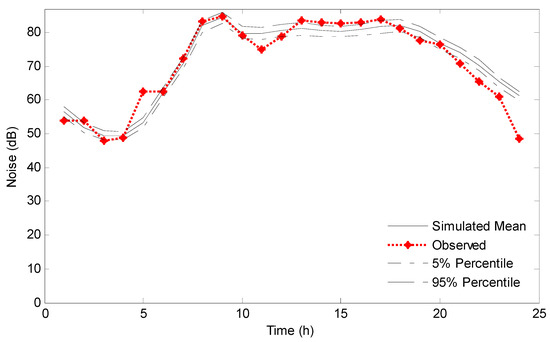
Figure 12.
Comparison between the predictions and observations in scenario B.
As can be seen from the green lines and red line in Figure 10b, the parameter values of Model (20) estimated from NEF are slightly different to those obtained from MLE. For example, the mean values of A and B obtained through NEF, as presented in Table 1, would be 4.7 and 28.7, respectively, while those values generated through MLE would be 5.2 and 26.8, respectively. However, even though there are differences between the parameter values obtained through NEF and MLE, the performance of NEF, with the value of R2 being 0.7691, is slightly worse than MLE (R2 value of 0.7699).
4.4. Parameter Estimation and Uncertainty Quantification of Traffic Noise Prediction Model at Scenario C
Scenario C corresponds to Site C, which is located on the road with old pavement from Albert St to Wascana Pkwy, as depicted in Figure 2. Figure 13 presents the initial and final results of Model (20). The initial uncertainty in Model (20) (indicated by the green lines in Figure 13a) would be significantly reduced through the NEF process (presented by the green lines in Figure 13b). The uncertainties in parameters A and B of Model (20) would also decrease, as shown in Figure 14, during the data assimilation process, and the final values of A and B can be compressed within small intervals (presented in Table 1 and Figure 14a,b). Figure 15 shows a comparison between the predicted intervals and observations in scenario C, indicating an acceptable performance of NEF.
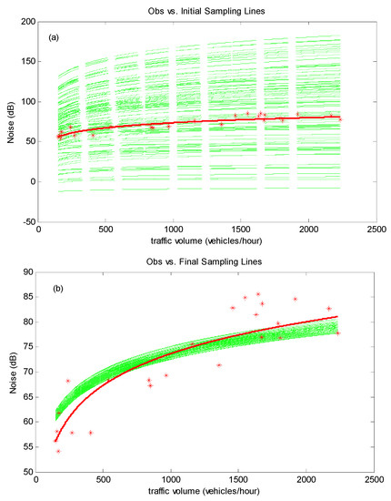
Figure 13.
Initial (a) and updated (b) traffic noise prediction curves in scenario C.
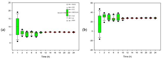
Figure 14.
Variations of parameters (a) and (b) in Model (20) during the data assimilation process under scenario C.
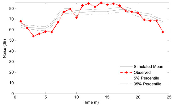
Figure 15.
Comparison between the predictions and observations in scenario C.
As can be seen from the green lines and red line in Figure 13b, the parameter values of Model (20) estimated from NEF are quite different to those obtained from MLE. As presented in Table 1, the mean values of A and B obtained through NEF would be 6.6 and 27.6, respectively, while those values generated through MLE would be 9.2 and 10.1, respectively. However, even though there are differences between the parameter values obtained through NEF and MLE, the performance of NEF, with the value of R2 being 0.8183, is better than MLE (R2 value of 0.7646).
5. Conclusions
- (1)
- A nested ensemble filtering (NEF) approach has been advanced for parameter estimation and the uncertainty quantification of traffic noise prediction. This improves upon the ensemble Kalman filter (EnKF) method by incorporating the sample importance resampling (SIR) procedures into the EnKF update process. Compared with the EnKF method, the proposed NEF approach can avoid the overshooting problem (abnormal value (e.g., outside the predefined ranges, complex values) in parameter or state samples) existing in the EnKF update process.
- (2)
- The proposed NEF approach was applied to traffic noise prediction on the Trans-Canada Highway in City of Regina. The traffic noise model is incorporated into the proposed NEF approach to quantify the parameter uncertainties in the traffic noise prediction model. Such a process is implemented using Matlab. Four scenarios at three observation sites were designed to evaluate the performance of the NEF approach in estimating unknown parameters and quantifying the uncertainty of the empirical traffic noise prediction model. Both new (scenarios A2 and B) and old (scenarios A1 and C) pavement condition were considered. The results demonstrate the applicability of the proposed methodology.
- (3)
- Comparisons between the nested ensemble filtering approach and maximum likelihood estimation (MLE) method have been undertaken. It is indicated that: (a) the NEF method performed better than MLE in most conditions, (b) the model parameters can be recursively corrected whenever new measurement is available, and (c) the uncertainty in the traffic noise model can be reduced well and quantified through the proposed NEF approach.
- (4)
- This study is a new attempt to improve upon the ensemble Kalman filter. Only the empirical traffic noise prediction model was applied to demonstrate the applicability of the proposed NEF method. It is desired that more real-world models (e.g., FHWA traffic noise model) will be undertaken to demonstrate the practical applicability of the proposed NEF method.
Author Contributions
Y.F. and L.D. designed the research; K.H. conducted the field measurements and calculation; K.H. and Y.F. wrote the manuscript; L.D. made the revision. All authors have read and agreed to the published version of the manuscript.
Funding
This research was funded by the Brunel University Open Access Publishing Fund.
Acknowledgments
We are very grateful for the editor’s and the anonymous reviewers’ insightful and constructive comments. They are critically helpful for improving this manuscript.
Conflicts of Interest
The authors declare no conflict of interest.
References
- Lercher, P.; Evans, G.W.; Meis, M. Ambient noise and cognitive processes among primary schoolchildren. Environ. Behav. 2003, 35, 725–735. [Google Scholar] [CrossRef]
- Basner, M.; Babisch, W.; Davis, A.; Brink, M.; Clark, C.; Janssen, S.; Stansfeld, S. Auditory and non-auditory effects of noise on health. Lancet 2014, 383, 1325–1332. [Google Scholar] [CrossRef]
- Sygna, K.; Aasvang, G.M.; Aamodt, G.; Oftedal, B.; Krog, N.H. Road traffic noise, sleep and mental health. Environ. Res. 2014, 131, 17–24. [Google Scholar] [CrossRef]
- Vienneau, D.; Schindler, C.; Perez, L.; Probst-Hensch, N.; Röösli, M. The relationship between transportation noise exposure and ischemic heart disease: A meta-analysis. Environ. Res. 2015, 138, 372–380. [Google Scholar] [CrossRef] [PubMed]
- Minichilli, F.; Gorini, F.; Ascari, E.; Bianchi, F.; Coi, A.; Fredianelli, L.; Licitra, G.; Manzoli, F.; Mezzasalma, L.; Cori, L. Annoyance Judgment and Measurements of Environmental Noise: A Focus on Italian Secondary Schools. Int. J. Environ. Res. Public Health 2018, 15, 208. [Google Scholar] [CrossRef]
- Huang, K.; Dai, L.M.; Fan, Y.R. Characterization of noise reduction capabilities of porous materials under various vacuum conditions. Appl. Acoust. 2020, 161, 107155. [Google Scholar] [CrossRef]
- Miedema, H.M.E.; Oudshoorn, C.G.M. Annoyance from transportation noise: Relationships with exposure metrics DNL and DENL and their confidence intervals. Environ. Health Perspect. 2001, 109, 409–416. [Google Scholar] [CrossRef]
- Abo-Qudais, S.; Alhiary, A. Statistical models for traffic noise at signalized intersections. Build. Environ. 2007, 42, 2939–2948. [Google Scholar] [CrossRef]
- Licitra, G.; Ascari, E.; Brambilla, G. Comparative analysis of methods to estimate urban noise exposure of inhabitants. Acta Acust. United Acust. 2012, 98, 659–666. [Google Scholar] [CrossRef]
- Licitra, G.; Fredianelli, L.; Petri, D.; Vigotti, M.A. Annoyance evaluation due to overall railway noise and vibration in Pisa urban areas. Sci. Total Environ. 2016, 568, 1315–1325. [Google Scholar] [CrossRef]
- Licitra, G.; Teti, L.; Cerchiai, M.; Bianco, F. The influence of tyres on the use of the CPX method for evaluating the effectiveness of a noise mitigation action based on low-noise road surfaces. Transp. Res. Part D Transp. Environ. 2017, 55, 217–226. [Google Scholar] [CrossRef]
- Praticò, F.G.; Fabienne, A.L. Trends and issues in mitigating traffic noise through quiet pavements. Procedia Soc. Behav. Sci. 2012, 53, 203–212. [Google Scholar] [CrossRef]
- Praticò, F.G. On the dependence of acoustic performance on pavement characteristics. Transp. Res. Part D Transp. Environ. 2014, 29, 79–87. [Google Scholar] [CrossRef]
- Licitra, G.; Cerchiai, M.; Teti, L.; Ascari, E.; Bianco, F.; Chetoni, M. Performance assessment of low-noise road surfaces in the leopoldo project: Comparison and validation of different measurement methods. Coatings 2015, 5, 3–25. [Google Scholar] [CrossRef]
- Licitra, G.; Moro, A.; Teti, L.; Del Pizzo, A.; Bianco, F. Modelling of acoustic ageing of rubberized pavements. Appl. Acoust. 2019, 146, 237–245. [Google Scholar] [CrossRef]
- Del Pizzo, A.; Teti, L.; Moro, A.; Bianco, F.; Fredianelli, L.; Licitra, G. Influence of texture on tyre road noise spectra in rubberized pavements. Appl. Acoust. 2020, 159, 107080. [Google Scholar] [CrossRef]
- Steele, C. A critical review of some traffic noise prediction models. Appl. Acoust. 2001, 62, 271–287. [Google Scholar] [CrossRef]
- Huang, K.; Dai, L.M.; Huang, W. Effects of Road Age and Traffic Flow on the Traffic Noise of the Highways in an Urban Area. J. Environ. Inform. 2014, 24, 121–130. [Google Scholar] [CrossRef]
- Peng, W.; Mayorga, R.V. Assessing traffic noise impact based on probabilistic and fuzzy approaches under uncertainty. Stoch. Environ. Res. Risk Assess. 2008, 22, 541–550. [Google Scholar] [CrossRef]
- Gimenez, A.; Gonzalez, M. A stochastic model for the noise level. J. Acoust. Soc. Am. 2009, 125, 3030–3037. [Google Scholar] [CrossRef]
- Ramirez, A.; Dominguez, E. Modeling urban traffic noise with stochastic and deterministic traffic models. Appl. Acoust. 2013, 74, 617–621. [Google Scholar]
- Iannone, G.; Guarnaccia, C.; Quartieri, J. Speed distribution influence in road traffic noise prediction. Environ. Eng. Manag. J. 2013, 12, 493–501. [Google Scholar] [CrossRef]
- Huang, K.; Dai, L.M.; Yao, M.; Fan, Y.R.; Kong, X.M. Modelling Dependence between Traffic Noise and Traffic Flow through An Entropy-Copula Method. J. Environ. Inform. 2017, 29, 134–151. [Google Scholar] [CrossRef][Green Version]
- Huang, K. Analysis of Impact Factors for Traffic Noise in Urban Areas. Ph.D. Thesis, Faculty of Graduate Studies and Research, University of Regina, Regina, SK, Canada, 2014. [Google Scholar]
- Plaze Guingla, D.A.; De Keyser, R.; De Lannoy, G.J.M.; Giustarini, L.; Matgen, P.; Pauwels, V.R.N. Improving particle filters in rainfall-runoff models: Application of the resample-move step and the ensemble Gaussian particle filter. Water Resour. Res. 2013, 49, 1–17. [Google Scholar] [CrossRef]
- Weerts, A.H.; EISerafy, G.Y.H. Particle filtering and ensemble Kalman filtering for state updating with hydrological conceptual rainfall-runoff models. Water Resour. Res. 2006, 42, W09403. [Google Scholar] [CrossRef]
- DeChant, C.M.; Moradkhani, H. Examining the effectiveness and robustness of sequential data assimilation methods for quantification of uncertainty in hydrologic forecasting. Water Resour. Res. 2012, 48, W04518. [Google Scholar] [CrossRef]
- Moradkhani, H.; Hsu, K.-L.; Gupta, H.; Sorooshian, S. Uncertainty assessment of hydrologic model states and parameters: Sequential data assimilation using the particle filter. Water Resour. Res. 2005, 41, W05012. [Google Scholar] [CrossRef]
- Fan, Y.R.; Huang, G.H.; Baetz, B.W.; Li, Y.P.; Huang, K.; Chen, X.; Gao, M. Development of integrated approaches for hydrological data assimilation through combination of ensemble Kalman filter and particle filter methods. J. Hydrol. 2017, 550, 412–426. [Google Scholar] [CrossRef]
- Fan, Y.R.; Huang, G.H.; Baetz, B.W.; Li, Y.P.; Huang, K. Development of a copula-based particle filter (CopPF) approach for hydrologic data assimilation under consideration of parameter interdependence. Water Resour. Res. 2017, 53, 4850–4875. [Google Scholar] [CrossRef]
- Saskatchewan Highways. Feature: East Regina TCH, Archived from the Original on 25 November 2006. Available online: https://web.archive.org/web/20061125064726/http://www.saskhighways.homestead.com/regina_TCH.html (accessed on 21 September 2006).
- Bérengier, M. Acoustical impact of traffic flowing equipments in urban areas. In Proceedings of Forum Acusticum; European Acoustical Association: Sevilla, Spain, 2002. [Google Scholar]
- Pierre, R.L.S., Jr.; Maguire, D.J. The impact of A-weighting sound pressure level measurements during the evaluation of noise exposure. In Proceedings of the Conference NOISE-CON, Baltimore, MD, USA, 12–14 July 2004; pp. 12–14. [Google Scholar]
- Harrison, M. Vehicle Refinement: Controlling Noise and Vibration in Road Vehicles, 1st ed.; Elsevier: Amsterdam, The Netherlands, 2004. [Google Scholar] [CrossRef]
- Pallas, M.A.; Lelong, J.; Chatagnon, R. Characterisation of tram noise emission and contribution of the noise sources. Appl. Acoust. 2011, 72, 437–450. [Google Scholar] [CrossRef]
- Faure, B.; Chiello, O.; Pallas, M.A.; Serviere, C. Characterisation of the acoustic field radiated by a rail with a microphone array: The SWEAM method. J. Sound Vib. 2015, 346, 165–190. [Google Scholar] [CrossRef]
- Pallas, M.A.; Berengier, M.; Chatagnon, R.; Czuka, M.; Conter, M.; Muirhead, M. Towards a model for electric vehicle noise emission in the European prediction method CNOSSOS-EU. Appl. Acoust. 2016, 113, 89–101. [Google Scholar] [CrossRef]
- Rao, R.P.; Rao, S.M.G. Environmental noise levels due to motor vehicular traffic in Visakhapatnam city. Acustica 1991, 74, 291–295. [Google Scholar]
- Singal, S.P. Noise Pollution and Control Strategy; Narosa Publication House: New Delhi, India, 2005. [Google Scholar]
- Agarwal, S.; Swami, B.L. Comprehensive approach for the development of traffic noise prediction model for Jaipur city. Environ. Monit. Assess. 2011, 172, 113–120. [Google Scholar] [CrossRef] [PubMed]


© 2019 by the authors. Licensee MDPI, Basel, Switzerland. This article is an open access article distributed under the terms and conditions of the Creative Commons Attribution (CC BY) license (http://creativecommons.org/licenses/by/4.0/).