Featured Application
The article gives a detailed description on how to implement a custom force control for collaborative robots without knowing all the internal parameters. The methodology presented can be used in any manufacturing process capable of being carried out by a collaborative robot.
Abstract
Due to the elasticity of their joints, collaborative robots are seldom used in applications with force control. Besides, the industrial robot controllers are closed and do not allow the user to access the motor torques and other parameters, hindering the possibility of carrying out a customized control. A good alternative to achieve a custom force control is sending the output of the force regulator to the robot controller through motion commands (inner/outer loop control). There are different types of motion commands (e.g., position or velocity). They may be implemented in different ways (Jacobian inverse vs. Jacobian transpose), but this information is usually not available for the user. This article is dedicated to the analysis of the effect of different inner loops and their combination with several external controllers. Two of the most determinant factors found are the type of the inner loop and the stiffness matrix. The theoretical deductions have been experimentally verified on a collaborative robot UR3, allowing us to choose the best behaviour in a polishing operation according to pre-established criteria.
1. Introduction
In the next few years, a significant increase in the number of industrial robots is expected. The prediction of the International Federation of Robotics (IFR) [1] is that between 2020 and 2022, nearly two million new industrial robots will be installed in factories around the world. However, despite this high demand, the robots are not useful for many manufacturing tasks today—in particular, those found in small and medium enterprises. A goal for the next generation of smart factory floors is to bring humans and robots closer together, working efficiently and collaborating safely [2].
Commonly, industrial robots are used in applications of low contact forces, such as material handling, welding, assembly, and painting. Nevertheless, in the last few years, industrial robots have been used in many applications of high interaction, such as milling, drilling, threading, and cutting. Also, they have been used to perform surface finish tasks such as grinding, brushing, polishing, and deburring [3].
On the other hand, the use of collaborative robots (cobots) has increased in recent years. The high productivity, flexibility, and quality of cobots, together with their low cost and high levels of safety, making them a perfect alternative in interaction tasks. However, the disadvantages of these robots are their lower stiffness compared with traditional ones. Their stiffness is lower because their joints usually contain harmonic drives. These have a safe and reliable power transmission with high reduction and low weight. However, they add more elasticity to the joints of the robot. The high force produced in the contact, combined with the low stiffness, generates deflections in the end effector, causing position errors and vibrations [4,5].
In the last few decades, many studies have been carried out in the area of force control using robots with elastic joints. One of the first relevant works [6] uses a corrective control for the singular perturbation model and the integral manifold technique to develop an inner/outer control. Where the inner loop is linearizing feedback control, and the outer loop can be implemented with the typical rigid robot force controls, as impedance control or hybrid position/force control. In the articles of Ren, T. et al. [7] and Ajoudani, A. et al. [8], the authors use the joint elastic torques to decouple the joint actuators and perform an impedance force control. The works in Magrini, E. et al. [9], Ahmad, S. [10] and Goldsmith, P. et al. [11] use a torque-controlled system to make a hybrid position/force control. Finally, a sliding mode control, adaptive control, and robust control have also been used as a solution to force control [12,13,14,15]. These techniques, in general, assume that the dynamic models of elastic joint robots are precisely known. Also, they assume the user can access the torques of the motors, which is not usually the case in commercial robots. Besides, the desired trajectory must be derivable at least four times, and the acceleration of the robot must be measured. However, in many commercial robots, the acceleration and the dynamic parameters cannot be obtained.
Other researchers have developed force controllers without knowledge of dynamics, such as the works found in Ma, Z. et al. [16] and Huang, L. et al. [17]. Nevertheless, the robot control with elastic joints requires measurements of the whole state of the system as the motor side angles, the link side angles, and the torque of the joints. These measures are difficult to get them in a commercial robot.
Commonly, commercial manipulators do not allow direct access to the actuator torques; therefore, a torque-based control cannot be used. However, most commercial manipulators have built-in position controllers. Some also have the possibility of velocity regulation. In these cases, it is possible to achieve a force control by using inner/outer controllers that consists of an inner position/velocity loop plus an outer force control loop. The external loop provides a reference position/velocity to the inner loop. Examples of inner/outer force control loops on rigid manipulators can be found in the works of Chiaverini, S. et al. [18], Winkler, A. and Suchy, J. [19], De Schutter, J. et al. [20] and Neranon, P. and Bicker, R. [21].
An advantage of the inner/outer loop is that this control does not need to know the dynamic parameters of the robot [20]. The errors in the dynamic model can be modelled as force disturbances.
Some researches apply the inner/outer algorithm directly to the robot motion control. This has the advantage of executing the task relatively straightforward [22,23,24], while others develop a macro-mini manipulator, where the robot is the macro manipulator, and a special end-effector is the mini manipulator or active device [25,26,27].
As collaborative robots are lighter and cheaper, the use of mini manipulators does not appear to be an available alternative. The mini manipulator requires the development of another and specific mini controller to each process. This method requires actuators, power amplifiers, active control devices, and algorithms. They are expensive and relatively difficult to implement. Besides, a specific device generates less stiffness and raise weight in the end effector [28].
According to the above, this article proposes the analysis and experimentation of a force control with an inner motion loop on collaborative robot arms. The methodology implemented allows us to demonstrate the possibility for cobots to perform a force control, although the internal parameters of the robot remain unknown. This work proves the application of these control in a polishing operation. Additionally, the analysis proposed considers the effect of the stiffness in the robot when it is used in force tasks with an inner/outer control loop.
This article is structured as follows. Section 2 presents the dynamic model for robots with elastic joints. Section 3 describes the inner/outer control loops with their advantages and drawbacks. Then, Section 4 shows an analysis of the possible inner loops and how the inner loops can affect the response of the force control. Section 5 shows the methodology, experimental platform, techniques used, and task planning. Section 6 exposes the results and discussion of the experiments performed with a commercial collaborative robot. In this section, the inner position loop and the velocity loop are compared. Besides, different algorithms for outer loops are contrasted. The best inner/outer loop is applied in a polishing task. Finally, Section 7 collects the conclusions.
2. Description of Dynamic Model for a Robot with Elastic Joints
Under the assumptions in Zollo, L. et al. [29], the dynamic model of a robot with elastic joints can be expressed as
where , , and are the vectors of position, velocity, and acceleration of links, respectively. , , and are the vectors of positions, velocities, and accelerations of motors. is the robot link inertia matrix, is the vector of centrifugal and Coriolis torques, is the diagonal matrix of joint stiffness coefficients, is vector of gravitational torque, and is a constant diagonal matrix, including the rotor inertia in the gear ratios. , , and contain, in this order, the viscous coefficient in the link side, the viscous coefficient in the motor side, and the damping of the elastic springs at the joints. is the input vector of driving torques, is the vector of contact force exerted by the end effector on the environment, and is the Jacobian matrix that relates joint velocities with the vector of end-effector velocities, . The Jacobian is assumed to be non-singular. The transpose of the matrix, , also relates the end effector force with the joint torques.
For analysis purposes, the environment is modelled as a frictionless and elastically compliant plane, which is very common in force control [18,29,30]. One contact point is considered, and the contact force is expressed as
where is the end-effector position, is the position at the contact point, and is the constant symmetric stiffness matrix of the environment.
3. Inner/Outer Control Loops
Among the main benefits of the force control with inner/outer loops are that the dynamics and kinematics of the robot are included through the inner loop. In addition, this control is easy to implement because only the outer control loop must be regulated. Also, sometimes, this control strategy is the only possible way to perform a custom force control.
On the other hand, the inner/outer loop has some disadvantages. There are limitations in the robot command set—for example, some robots do not have velocity commands. There is a lack of information about the inner loop, control type, and control parameters. There is no possibility to access the input of the torques directly, which makes it impossible to implement a force control in a robot that applies inverse dynamic methods [6,9,31].
The stiffness of the environment is a very important factor in the performance of the interaction tasks. Therefore, it is necessary to know this parameter to have better force control.
The sampling period of the inner loop, established initially for position control, could be too slow for force control. Some functions necessary for control (e.g., the Jacobian matrix) cannot be implemented using the set of commands. Due to the sampling period, if the external loop is implemented through an external computer, there will be communication delays.
The general block schemes of the typical configurations of inner/outer loops, with an inner position loop and an inner velocity loop, are shown in Figure 1. The force of environment measured with the force sensor is compared with the desired force . After that comparison, force error is generated. This error is used by the force controller to produce the reference of absolute position (Figure 1a), incremental position (Figure 1b), or velocity (Figure 1c).
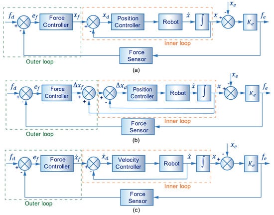
Figure 1.
Force control with inner motion loops (a) with inner absolute position loop, (b) with inner incremental position loop, and (c) with inner velocity loop.
In the three schemes, it has been assumed that the internal controller compensates nonlinearities of the process. In the diagrams, the only difference between position and velocity lies in the integrator, which is not included in the inner loop for the velocity controller. However, there are crucial differences not reflected in the graphs.
The parameters of the controllers can differ for position and velocity control. Thus, it could be necessary to implement different external loops depending on the inner controller. Also, the stiffness matrix is not the same in the three cases.
The external force loops are not limited by the set of motion commands of the robot. In recent decades, many authors proposed several types of general algorithms for outer loops. Table 1 shows some of the most relevant, where is the control action applied over the inner loop, and are the reference and measured force, respectively. and are the reference and measured derivative force, respectively. , , and are the gain matrices of the proportional, derivative, and integral control, in this order. is the gain matrix of the velocity feedback damping, is the cartesian velocity, and is the feedforward action.

Table 1.
Typical control action for outer force loops.
As can be read in Neranon, P. and Bicker, R. [21], PD and PID controls are usually replaced by a PV or PIV controls due to the high noise produced by the force sensor, which makes the use of a derivative control impracticable.
As it is known from control theory, the integral control action guarantees zero error if the system is stable. However, it brings some problems like potential stability loss, wind-up, and slow convergence. Additionally, in force control, if the sampling period is slow, the integrator does not eliminate the error, as it will be demonstrated in the experimental part of this paper. For these reasons, the use of an integrator should be considered for every case.
One of the main problems in force control is the change from free to constrained movement. This transition phase, also called impact, is probably the most critical part of the task. This difficulty could lead to the need for the use of different regulators in each phase. In Zotovic, R. and Valera, A. [32], a single valid controller for force control and impact control is proposed. First, the controller is set to perform speed control in free movements and force control in constrained movements. It avoids the need to switch regulators and their associated problems. Second, they proposed switching off the proportional constant and the feedforward to attenuate the impact. Therefore, the stability of the system is improved through a better dissipation of energy.
In Siciliano, B. et al. [33], researchers studied two cases of external loops for different inner loops. For an inner position loop, the authors proposed an external PV force controller. For an internal velocity loop, the authors proposed just a proportional, P, force control for the outer loop. The authors deduced that a proportional regulator of external force, with a proportional regulator for the inner velocity loop, reaches the reference force in a finite time. However, this does not happen with the inner regulator by position. For this reason, it is necessary to add an integrator in the force loop. It is known that this reduces bandwidth and stability margin.
4. Analysis of Inner Motion Loops
The inner loops are implemented inside robot controllers. In most commercial robots, the details, such as dynamics parameters, gains, and algorithms of the inner controller, are not available for users. However, today, most of the robot controllers compensate for the nonlinear dynamics or, at least, the effect of gravity. The force control tasks are usually performed at very low velocities and accelerations. Thus, the inertia, centrifugal, and Coriolis forces have less influence than gravity force.
As stated previously, the inner control may be a position loop or a velocity loop. Several authors have used different forms of inner loops. All of them had to use Cartesian commands. Some used absolute position commands [21,34]. Zeng, G. and Hemami, A. [35] used position increments instead of absolute positions, and in the works of Magrini, E. et al. [9] and Han, D. et al. [30], the authors used inner velocity loops. It should be emphasized that some robot controllers do not have cartesian velocity commands, so this option is not always available.
An essential feature for the force control in a robot is the cartesian stiffness matrix. This matrix determines the deviation of the robot from the nominal trajectory, under the effect of external forces. The expression for this matrix depends on several factors. First, it is influenced by the location of the position/velocity sensor for the feedback of the inner loop. It may be located on the motor (a typical configuration for rigid robots) or on the link (for the elastic ones). The cartesian stiffness matrix is not equal in all the working range of the robot. It may be essential to know the expression for the stiffness matrix to deduce where to perform the task, what will be the errors, etc.
Another important factor is how the inner loop coordinate transformation is performed. The force control must be programmed in cartesian space. However, the motors are controlled in joint space. Thus, cartesian coordinates must be transformed into joint coordinates. This can be implemented in two ways, through the Jacobian inverse method or the Jacobian transpose method. Thus, the control action of the inner position loop can be computed with these two methods by the robot controller [33].
In the first case, the first step is to compute the cartesian position error and use the Jacobian inverse to transform it into joint coordinate errors. Then, the control action is carried out. In the second case, the regulator is applied directly to the cartesian position error. The result is multiplied by the Jacobian transpose to obtain the input torques of the motors. These two possible configurations, called Jacobian inverse control and Jacobian transpose control, can be seen in Figure 2.
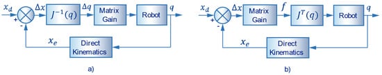
Figure 2.
Block schemes of operational space control (a) with Jacobian inverse and (b) with Jacobian transpose.
In Section 4.1, the cartesian stiffness matrix is analysed depending on the location of the position/velocity sensor, and the type of inner loop. Section 4.2 will study the effect of different combinations of inner and outer loops, as well as the way they communicate. The external loops were given in Equations (6)–(10). The inner loops will be position and velocity, both with Jacobian inverse and Jacobian transpose. For the position inner loop, cases of absolute and incremental positions will be considered. For each one, the steady-state error and stiffness matrix will be deduced.
The analysis of the inner loops allows to understand how they can affect the force response, and in this way, to deduce what inner loop should be applied in the robot to ensure better performance in the interaction task.
4.1. The Stiffness Matrix
In force control, the interaction forces may cause deviation of the end-effector from the nominal trajectory. There are two different reasons. First, the external forces produce mechanical deformation of the gears. Second, the external forces induce a deviation of the motors from their reference path. The first case depends on the mechanical robustness of the robot. The second case depends on the controller.
The mechanical deformations occur in joint space. Regarding the controller, it can be implemented in both joint and cartesian space. The effect on the error will be different in the two cases.
The joint stiffness matrix is defined as the relation between the deformation of the joints and the applied torque,
where is the vector of motor torques, is the diagonal stiffness matrix, and is the vector of differences between actual joint and reference positions.
The force control tasks are programmed in the cartesian space. Thus, for a good performance, it is crucial that the robot deviates from the nominal cartesian trajectory as little as possible. The cartesian stiffness matrix describes the relationship between the deformations and the force in all the cartesian directions. It is highly recommended to have higher stiffness in order to avoid errors. The opposite phenomenon of stiffness is called compliance.
The robot cartesian stiffness matrix, , was first introduced in Salisbury, J. [36] as
where and are the Jacobian transpose and Jacobian inverse, respectively.
Next equation relates the cartesian position deviations and the external force vector,
It should be noted that the Jacobian matrix of the robot depends on its position and, therefore, the cartesian stiffness matrix, too.
In reference [37], researchers introduced the conservative congruence transformation—Equation (14)—giving an improved version of the cartesian stiffness matrix,
where is the additional stiffness term, caused by the variation of the Jacobian matrix and the external force vector.
The part of the stiffness due to the mechanical deformation of the gears is called passive stiffness. It is always expressed in cartesian space. In this study, it is referred as joint stiffness. The part due to the deviations of the motors is called active stiffness and can be modified by the adequate adjustment of the controller. It can be expressed in cartesian or joint space, depending on the way the control is made.
The works of Salisbury, J. [36] and Chen, S. and Kao, I. [37] were made for classical, rigid robots. These robots usually have only one position sensor per motor. It is located on the motor side and not in the link because the measured position has a higher resolution. It is assumed that the position of the motor and the link are equivalent. It is considered that there is no deformation of the gears, which may be corrected by the position control. However, in force control tasks, the deformations cannot be neglected.
On the other hand, the robots with elastic joints usually have two position sensors (encoders) [38]. The first encoder is on the motor side, and the second one is on the link side, as shown in Figure 3.

Figure 3.
The joint module of the Light WeigthRobot III, adapted from Institute of Robotics and Mechatronics of German Aerospace Center (Deutsches Zentrum für Luft-und Raumfahrt-DLR) [38].
This way, it is possible to control as feedback the position of the motor or the position of the link. Besides, the motor or the link velocities can be controlled, too. Thus, there are several possibilities: motor position control, motor velocity control, link position control, link velocity control, or a combination of them.
4.1.1. Motor Position
Considering the robot dynamics, Equations (1) and (2) in a steady-state and an input control in the motor side, we have
where is the desired motor position, and is the proportional gain matrix of the motor position control. Solving for from Equation (16),
Replacing (17) in (15) and solving for , we have
Therefore, the link positions will be affected by an equivalent stiffness that is influenced by the passive stiffness, , and the active stiffness of the motion control, . Since the motor and link positions are equivalent and assuming the reduction factor , we can consider that . For small deformations, and can be related,
Then, the cartesian stiffness matrix is
Hence, in this case, the active and passive stiffnesses are equivalent.
4.1.2. Link Position
Considering the robot in a steady-state and input control (position sensor) in the link side, we have
where is the desired link position, and is the proportional gain matrix of the link position control. Solving for from Equation (22),
therefore, the link positions will be affected only by the active stiffness of the joint motion control, . The stiffness matrix will be
4.1.3. Link Velocities
In the case of link velocity control, there is a possibility of finding stiffness effects depending on the type of control. Considering the control input, as a proportional-integral with gravity compensation, ,
where is the desired link velocity, is the proportional gain matrix, and is the integral gain matrix of the velocity control.
The integral term can be analysed as a proportional term regarding the position.
Considering the robot dynamics, Equations (1) and (2) and the input in a steady state, we have
Solving for from Equation (29),
Ordering the equation,
Hence, the cartesian stiffness matrix of the robot will be,
The term acts like a bias. It means, for zero external force , the robot will have some deformation. Therefore, the integral control acts like active stiffness and the proportional control as a bias. If the velocity loop does not have an integrator, just like a proportional control, the control action will be.
The first term acts like bias and the second one as damping. Thus, there is no active stiffness. The system will behave like a mass-damper under an external force. The final state will be achieved when the robot stops (.
which means, that the reference velocities, , should be
This corresponds to an open control loop, theoretically without force error.
In summary, if the velocity loop has an integrator, the integrator acts like active stiffness in the joint space and the proportional control as bias. In the case, it does not contain an integrator; if no stiffness term appears, then the exerted force is proportional to the reference velocity.
4.2. Absolute Cartesian Position Inner Loop
In the following subsection, we will make the convergence analysis of the force for the case when the external loop sends the absolute reference position to the controller. In the deduction, we will use the proportional-derivative and the proportional-derivative with feedforward as external loops. The proportional-integral-derivative will not be studied since it guarantees zero error if the system is stable.
Regarding the inner loops, both possibilities—Jacobian inverse and Jacobian transpose—will be contemplated. Every combination of inner and outer loop will be studied. The deductions of the formulae will be omitted for briefness. Only the final results will be presented.
4.2.1. Jacobian Transpose
Considering the motion control as PV with gravity compensation. In this case, the error is in cartesian coordinates. Thus, the input torque is
where is the proportional gain matrix in cartesian space.
Replacing Equation (37) in dynamics, Equations (1) and (2), and resolving for steady-state force , the following expression is obtained:
The force will be influenced by the passive stiffness of the environment, , and the active stiffness of the motion control, , as well as the position of the environment, . Typically, these values are unknown. However, the value of is uniform in all the working range of the robot.
4.2.2. Jacobian Inverse
In this case, the error is in joint coordinates. Therefore, the inner control torque input is
where is the gains matrix of the proportional control in the joint space.
Replacing Equation (39) in dynamics and resolving for steady-state force, we have
where is the active stiffness in cartesian space, which is calculated through the coordinate transformation expressed in Equation (12).
The force will be influenced by the passive stiffness of the environment, , and the active stiffness of the motion control, , as well as the position of the environment, . Typically, these values are unknown. However, the value of is not uniform in all the working range of the robot.
4.2.3. Implications
The main difference in these methods is that the Jacobian inverse matrix, , and Jacobian transpose matrix, , appear in the term due to the transformation of the active joint stiffness into the cartesian space. This transformation of coordinates implies that the Cartesian stiffness depends on the actual position where the robot is, so it will not be constant during a given trajectory.
It should be noted that the force also depends on the input reference coming from the possible outer loops. Therefore, in Table 2, the final value of the steady-state force, , in both cases, is obtained by replacing with one of the outer algorithms already exposed in Table 1.
Table 2.
Response force of the control force with absolute position inner loop.
Here, is the selection matrix of the force direction, is the compliance matrix of the force control, and is the identity matrix.
The feedforward of the reference force eliminates the error in rigid robots, which have the possibility to access directly to the motor torques. However, the elasticity of the environment and the inner loop introduce an error. For the case of Jacobian transpose, to obtain zero error, the feedforward should be
and for the case of the Jacobian inverse,
In Table 2, the final value for the steady-state force depends on the characteristics of the environment, as its position ( and stiffness (. Thus, there will be a force error in steady state, unless those values are known with exactitude to be compensated.
It is crucial to notice that, in outer loops with feedforward action, it is possible to obtain a zero-force error. To achieve this, the reference force must have the value given by term. In the case of Jacobian transpose, the feedforward action depends on the environment and the proportional gain of the cartesian position control. In the other case (Jacobian inverse), the control action depends on the environment, and the proportional gain of the joint control transformed into cartesian space. Therefore, it is necessary to know the Jacobian matrix to calculate the stiffness in each sampling period. In summary, in all the versions of the absolute cartesian position control, the characteristics of the environment (stiffness and position) appear. To achieve good tracking, these magnitudes must be known. Moreover, for the inner loop with Jacobian transpose, the force control is uniform in all the working range. For the Jacobian inverse, it is not.
4.3. Incremental Cartesian Position Inner Loop
In the case of cartesian position control, we have another alternative to give a reference to the control. We can give the incremental difference instead of .
4.3.1. Jacobian Transpose
The calculated steady-state force depends on the product of the gain matrix of the cartesian proportional control and the desired incremental position.
4.3.2. Jacobian Inverse
In this case, the calculated steady-state force depends on the product of the gain matrix of the joint proportional control transformed into cartesian space and the desired incremental position.
4.3.3. Implications
As in the case of absolute position loop, in the Jacobian inverse method, the stiffness matrix must be determined through the transformation of the proportional gain from the space of the articulations into the cartesian space of the end effector. However, it should be noted that, in an incremental position loop, the force will not be affected by environmental conditions.
Table 3.
Response force of the control force with incremental position inner loop.
Here, is the selection matrix of the force direction and is the active compliance matrix of the force control.
The force control with incremental position loop depends only on the active stiffness of the position control, or , and the active stiffness of the force control, . Besides, the feedforward action is easier to implement because it only depends on the gains of the position controls. For the case of Jacobian transpose, to obtain zero error, the feedforward should be
and for the case of the Jacobian inverse,
In summary, the incremental position control has an important advantage over the absolute position control; it does not depend on characteristics of the environment.
4.4. Cartesian Velocity Inner Loop
In the case of the inner velocity loop, the input is considered as a proportional control with gravity compensation.
4.4.1. Jacobian Transpose
In this case, the input of the inner loop in the cartesian space is
where is the proportional gain matrix of the velocity cartesian control.
Replacing Equation (55) in dynamics and resolving it for steady state, we can calculate the force as the product of the proportional gain matrix and the desired velocity as
4.4.2. Jacobian Inverse
In this case, the input in the inner control is expressed in joint space. Thus, the input is
where is the proportional gain matrix of the velocity joint control.
Replacing Equation (57) in dynamics and resolving it for steady state, we can calculate the force as the product of the proportional gain matrix of the joint control (transformed into cartesian space) and the desired velocity,
As can be seen in the Equations (56) and (58), the force in steady state depends only on the active stiffness of the velocity control. In Equation (56) depends on the cartesian stiffness, , and in Equation (58) depends on the joint stiffness and the position of the robot due to the Jacobian term .
4.4.3. Implications
The results of the force obtained replacing by the algorithms exposed in Table 1 are shown in Table 4.
Table 4.
Response force of the control force with inner velocity loop.
Here, is the selection matrix of the force direction and is the compliance matrix of the force control.
In both cases, incremental position and velocity loop, it is possible to observe that control with feedforward action will only depend on the gain of the controller and will not depend on the position and stiffness of the environment. For the case of Jacobian transpose, to obtain zero error, the feedforward should be
and for the case of the Jacobian inverse,
Moreover, if the velocity control is a proportional-integral control, the force error in steady state will be zero.
Summarizing, the incremental position control and the velocity control are very similar. However, in real robots, they may behave in different ways. There are two main reasons for this. In one case, the inner loop uses the position proportional constants, while in the other case, it uses the velocity proportional constants. There is no reason why they should be equal. Thus, the active stiffness in one case will be higher than in the other. The other reason is that one of the inner loops (position or velocity) may use Jacobian transpose, while the other applies Jacobian inverse.
5. Methodology
The previous deductions have been verified experimentally. Different control methods have been tested and compared in practice. With these results, the best combination of inner and outer loop has been identified. These experiments were carried out through polishing operations.
5.1. Experimental Setup
The physical system employed in this study is shown in Figure 4. The robot used for the experiments is a UR3 (Universal Robots A/S, Odense, Denmark). This robot arm has a six-revolute-joints anthropomorphic geometry. The joints are actuated by servo motors via harmonics drive reduction; two encoders are used in each joint. A magnetic encoder monitors the motor position, and an optical encoder monitors the link position. A force sensor is mounted on the end effector of the robot.
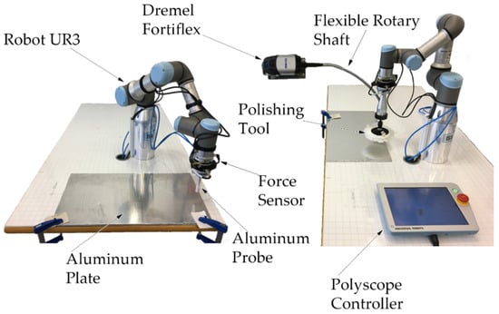
Figure 4.
Experimental setup.
The robot has a sampling frequency of 125 Hz or, in other words, a sampling period of 0.008 s. The force/torque sensor is type HEX-EB165 (OnRobot A/S, Odense, Denmark), with a force range from 0 N to 200 N and a torque range from 0 Nm to 10 Nm. The sensor has a maximum sampling frequency of 500 Hz and is directly connected with the robot controller. All the variables, such as position, velocity, torques, and forces, are sent via ethernet to a computer, where the data are received every sampling period by an acquisition software implemented in Labview (version 2017, National Instruments, Austin, TX, USA). Afterward, these data are processed with Matlab (version 2019, MathWorks Inc., Natick, MA, USA).
The preliminary experiments were made using an aluminium probe with a spherical tip attached directly to the force sensor to avoid vibrations. The definitive experiments were made with a common polishing tool.
Two materials were considered as workpiece—aluminium and a polymer plate—with the aim to evaluate the force control with different stiffness of the environment.
The tool chuck was driven by a Dremel model FortiFlex 9100 (Dremel Europe, Breda, The Netherlands) with a flexible rotary shaft. It was installed in the end-effector of the robot through a custom machined coupling. The final tool was a commercial polishing tool of 130 mm of diameter. It was composed of a rubber base and a buffing pad.
5.2. Method
To avoid the experimental comparisons of all the combinations of inner and outer loops, in the first step, we identified the internal loop with the best performance. For these experiments, we used a proportional force controller for the external loop. As demonstrated later in this paper, the best results were obtained with an inner velocity loop. In the following step, the behaviours of several external regulators were compared. The best inner loop identified in the first step was applied.
Regarding the identification of the optimal inner loop, in this work were considered the position and velocity loops in cartesian space. In the case of the position, both proposals, absolute and incremental, were treated. Also, in all the cases, the stiffness was evaluated.
Next, we explain the commands used to implement the inner loops. In the case of position loops, we used the command script movel,
where x vector represents the cartesian position to be reached by the end-effector, a is the acceleration, v is the velocity, t is the time, and radius is the blend radius. This command controls the position in the cartesian space in each sampling period. If the variable time is specified, the command will ignore the velocity and acceleration values. In our case, it was necessary to specify a time of 8 ms as a sampling period. Also, it was necessary to implement an external trapezoidal trajectory generator to specify the velocity and acceleration of the movement on the Y-axis. This trajectory generator was implemented with script commands.
movel(x vector, a, v, t, r).
In the case of the velocity loop, we used the command script speedl,
where v vector represents the cartesian velocity to be reached by the end-effector, a is the acceleration, and t is the time. This command controls the velocity in the cartesian space. We can indicate a specific cartesian velocity in each degree of freedom. However, we only can indicate a global acceleration. In this case, it was not necessary to specify the time because the command was applied in each sampling period.
speedl(v vector, a, t).
Then, the inner loop with the best performance was used with different outer force loops. A comparison between PD and PV algorithm is shown to study the effect of the damping action in the interaction task. In addition, the integral control action is compared with the feedforward action, in order to study which alternative is more appropriate in practical applications. All these results were obtained using the aluminium probe tool to avoid the vibrations of a real polishing tool.
Finally, a real application is shown. A polishing task was performed with the polishing tool and with the best force control obtained. The task was performed with and without the force control to compare results. The gains, applied in the different control algorithms, were determined experimentally. These values were found after several experiments and analysis of the force response. The best values of these gains are exposed in this work.
5.3. Task Planning
The trajectory of the task used in the experiments had initially a free movement in the minus Z direction with constant speed, switching to force control in the Z direction when the measured force surpassed a threshold of 1 N. The impact control consisted of a proportional gain of less value until reaching the reference force (5 N or 10 N). When the force reference was reached, the robot started a controlled movement on the Y direction, maintaining the pressure force over the workpiece surface. A scheme of the experiments is shown in Figure 5.
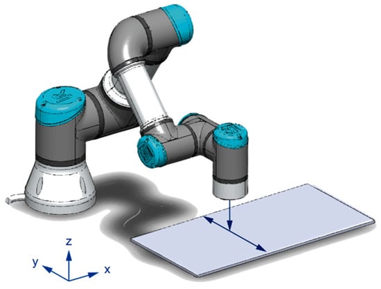
Figure 5.
Scheme of experiments.
5.4. Stiffness Parameters Identification
The stiffnesses of the joints were identified experimentally. The robot was stopped while the controller was working. Then different weights of 2 kg, 2.5 kg, and 3 kg were applied on the joints of the robot. The joint torques and joint positions were measured in the robot. The stiffness of each joint was calculated through Equation (65). The stiffness values of the joints are shown in Table 5.
where, for each joint, was the change in the torque value due to the added weights and was the change in the position value. As the joints of the UR3 robot have only three sizes [39], it was not necessary to measure the six joints. Base joint and shoulder joint have the same size, the elbow joint has the other size, and the three wrist joints have another same size. Then, it was only necessary to identify joint 5 (wrist), joint 3 (elbow), and joint 2 (shoulder). The three weights were applied to each joint and the stiffness values were obtained through the mean of the measurements.
Table 5.
Stiffness joint parameters.
6. Results and Discussions
6.1. The Inner Loops
6.1.1. Absolute Position Loop
In Section 4, it was demonstrated that the performance of the absolute position loop depends on the characteristics of the environment much more than the others. The worst results were expected from this loop. This hypothesis was confirmed by the experiments.
The output of the external loop corresponds to the reference position of the robot. In some cases, this position was not in contact with the environment, which provoked bouncing. High accelerations were reached. Sometimes, the robot had hard impacts against the piece, and the security measures were activated, causing an emergency stop.
After several experiments, this type of inner loop was discarded. It was the worst of three.
The plots resulting from these experiments have not been shown in the article. However, we included this method since we consider that our experience, albeit negative, may be useful to other people that work in force control.
6.1.2. Incremental Position Loop
Figure 6 shows the force control with an inner position loop applied over two materials: a polymer (orange lines) and aluminium (blue lines). As can be seen, the force response remains around the reference force of 5 N for the first 150 s. Concerning the material in contact, the force shows higher deviations in the aluminium as a result of seizing between same materials.
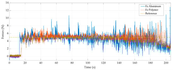
Figure 6.
Force control with inner position loop.
The force error at the end of the stroke (from 150 s) is mainly due to the changes produced in the cartesian stiffness. This suggests that the position loop is made with the Jacobian inverse method; therefore, the stiffness changes due to the change in position and the use of the Jacobian matrix.
A representation of the cartesian stiffness during the trajectory is shown in Figure 7. It was calculated using the coordinate transformation in Equation (12). In the figure, the force and stiffness in the Z direction, , are shown. As can be seen, during the time that the end effector is within the stable force path, at 5 N, the stiffness has the maximum value. However, when the robot is near the end of the trajectory, the stiffness decreases, generating errors in the force response. If the internal control gains were known, this effect would be compensated in the control action to avoid the observed deviations.
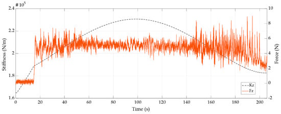
Figure 7.
Stiffness analysis in the inner position loop.
6.1.3. Velocity Loop
Figure 8 shows the force control with the inner velocity loop applied over the polymer (orange line) and aluminium (blue line). As can be seen, unlike the position loop, in the speed loop, the force is maintained around the reference value throughout the trajectory. Furthermore, it should be noted that there is no significant difference in the force error between materials. This coincides with stated in Equation (57), which indicates that the force response does not depend on the environment stiffness.
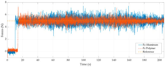
Figure 8.
Force control with inner velocity loop.
In addition, the velocity loop is not affected by the position in the trajectory of the robot. This allows to obtain better results, independently of the position of the robot in the workspace. This suggests that the velocity loop is implemented with the Jacobian transpose.
6.2. The Outer Loops
This subsection describes the experimental comparative analysis of the several external loops explained previously. The internal loop used in all the cases was the velocity loop, which demonstrated the best results.
In force control is not only important tracking the reference force. The oscillations and peaks of the applied force cause not only uneven polishing but also, a gradual deterioration in the robot mechanics. For these reasons, this work presents the average force tracking error, standard deviation, number of peaks, and maximal/minimal value to compare the different external loops.
6.2.1. Proportional Derivative (PD) vs. Proportional with Velocity Feedback (PV)
In Figure 9, we can observe the function of the force derivative (blue lines) and the velocity feedback term (yellow lines). The proportional algorithm P (orange lines) is used as a reference to compare the performance of the other algorithms.
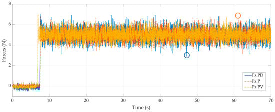
Figure 9.
Proportional derivative (PD) vs. proportional with velocity feedback (PV) comparison.
Regarding the response, the classic derivative action of the force control does not present good results due to the noise in the sensor, which worsens the numerical derivation, generating peaks up to 34% higher (highlighted as circles) than the pure proportional controller. This is due to the noise of the sensor and the long sampling period. Thus, the force derivative may change substantially during a sampling period.
Through the numerical results associated with the graph, the derivative control action employing the velocity feedback (PV) shows a slight improvement in damping peak force by 30%, and the PD peaks have a smaller size than in PV and P controls. However, the velocity changes faster than the sampling period, so its effect is not so observable.
6.2.2. Integral Action (PI) vs. Feedforward Action (P + FF)
In Figure 10, we can observe the function of the integral action and the feedforward of the force to reduce the error of the system.
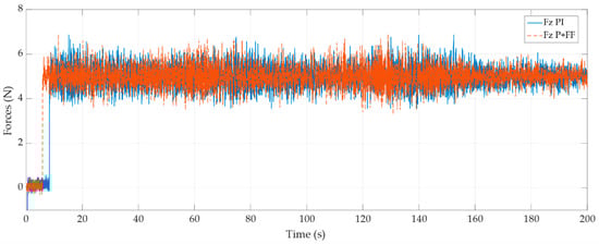
Figure 10.
Integral action (PI) vs. feedforward action (P + FF) comparison.
Although theoretically, the integral action guarantees a null error, it is not very popular, because it can have stability problems, wind-up, and slower convergence than a feedforward action.
On the other hand, control with feedforward is challenging to implement since it requires knowledge of the active stiffness matrix of the position control. In this case, we consider a constant gain for the feedforward action.
Due to the low sampling period and the fast dynamics of the interaction, both the integral action and the feedforward action do not guarantee a zero error. However, even using a constant feedforward, like the one used in Figure 10, P + FF allows to reduce the error from 0.11% to 0.02%.
6.2.3. Global Results
Table 6 contains the results of force control with velocity inner loop and with various types of outer loops. It should be noted that , , , and are the gains of the outer force loops. The table shows the mean, standard deviation, and the error respect to the reference value of 5 N. Also, it incorporates the maximum and minimum values reached by the force control. Finally, the quantity of picks outside the range of ±1 N are shown.
Table 6.
Comparison of outer loops.
Table 6 represents the value of the best experiments for every regulator (outer loop). It may be appreciated that the error is very small for all the outer loops.
According to the theory, PV should be more damped than a simple proportional, albeit it is slower to converge. According to the experiments, PV control has a slightly worse average error and standard deviation. However, it has fewer peaks, and they are lower. In the same way, a PD algorithm is applied. The results show as the derivative action in the force is worse than the feedback velocity action.
The smallest average error is obtained with P + FF control. However, PI and PIV have better standard deviation and fewer peaks outside the range of ±1 N. It should be emphasized that the feedforward term was constant in these experiments. The results can be improved by adjusting the feedforward gain based on the stiffness matrix.
Due to the number of criteria that determine the performance of force control, a prioritization matrix has been made. The aim of this matrix is determining the most suitable algorithm for the outer loop. The criteria for evaluating the algorithms are
- A mean close to the reference force;
- A minimum standard deviation;
- Fewer peaks above and below the reference force;
- Lower value of maximum and minimum force.
Furthermore, it is preferable to use algorithms where the adjustment of the gains of the force control is not dependent on the knowledge of the features of the inner loop.
Table 7 presents a prioritization matrix where the different algorithms are evaluated according to the criteria above. The weights of the criteria were previously determined, these weights should be decided according to the final application (in this case, a polishing task). The options were evaluated with a score from 1 to 5, with 5 being the best score.
Table 7.
Prioritization matrix of outer loops.
The total scores indicate that the use of a PIV algorithm is the most suitable option for this example. However, the P + FF algorithm is also a good option if the inner loop structure is known.
6.3. Polishing Application
A polishing task was performed to demonstrate the effectiveness of the force control. In Figure 11 and Figure 12, the force measurements for polishing with a reference force of 5 N and 10 N, are presented. For these experiments, we used an inner velocity loop with an outer PIV force loop. The figures display the measured cartesian forces, the reference force, and the force in Z—direction without force control.
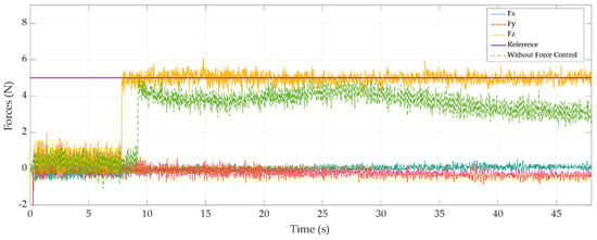
Figure 11.
Polishing with force control with reference force 5 N.
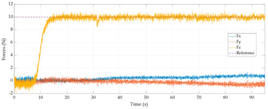
Figure 12.
Polishing with Force control with reference force 10 N.
In both cases, the force remains stable in both experiments. Forces and are shown. The force was produced by the friction along the trajectory. The force was produced by the radial force due to the polishing tool. It can be seen as the force and increase if the force increases.
As can be observed, the force response is better with the polishing tool than with the probe. This proves that the inner velocity loop is affected by the stiffness of the tool. Further, in Figure 11, it is possible to observe the polishing task without force control (green line). This demonstrates that without external force control is not possible to maintain the reference force. Thus, we obtain a poor surface polish. Table 8 shows the result of the polishing task.
Table 8.
Results for polishing task.
Table 8 includes values of mean, standard deviation, and error of the force control. Also, since the polishing tool is more flexible, it allows to obtain smaller measurement errors than the reference. This effect is reflected in the fewer number of observed picks.
7. Conclusions
In summary, the main goals have been achieved. An analysis of inner and outer control loops has been made, working with equations oriented to collaborative robots, unlike the proposals made for rigid robots [18,19,20,21]. The study was made with a practical approach to identify the inner loops when their characteristics are unknown. This is easier to implement than the works in Ma, Z. et al. [16] and Huang, L. et al. [17] because they measured all the variables of the robot, like torques, motor position, etc. The article also explains how that information may be used to define the external loop in order to obtain better results. The importance of the concept of the stiffness matrix, applied to robot control, has been proved in theory and practice.
After completing the previous steps and making experiments, the absolute position inner loop obtains the worse results. Theoretically, the incremental position loop and the velocity loops are equivalent. However, in practice, this equivalence depends on the way the internal loop is implemented and the gains of the inner control.
According to the way of the coordinate transformation is made by the robot controller (Jacobian transpose vs. Jacobian inverse), the stiffness matrix changes considerably. The Jacobian transpose gives a constant stiffness matrix, which causes stable contact force in all the working area of the robot, while the Jacobian inverse method gives a cartesian stiffness matrix that depends on the joint stiffness and the position of the robot.
As a rule, the user does not have the information on the way the inner loop was implemented. However, it can be deduced experimentally. To prove this, an experimental verification was made with a UR3 CB3 robot. Despite the limitations of this robot (as slow sampling frequency and low joint stiffness), the theoretical results have been mostly verified.
Summarizing, the results on the UR3 robot show that the variations in the performance of the different external controllers are small. Using a PV over a proportional (P) in the outer loop improves the impacts, while the PD action confirms a worse performance in force control, as observed in the paper of Neranon, P and Bicker, P. [21]. A feedforward term (FF) achieves better force tracking than an integrator (PI)—in this case, it is an improvement compared to the methods exposed in the book Siciliano, B. et al. [33]. However, it has more peaks. It may be enhanced if the stiffness matrix is introduced. Regarding the inner control, the inner velocity loop gives the best results, probably because it is implemented using the Jacobian transpose in the UR3.
The force control is affected by the stiffness of the tool, as is the case with the polishing tool, where its more flexible material lets reducing the number of oscillations obtained during the execution of the task. This fact decreases the effect of the problem explained in Iglesias, I. et al. [3].
Several problems remain for future works, and three stand out. Experiments should be repeated with a robot with better performance, such as increased joint stiffness and a faster sampling period, to prove their influence in the improvement of the force control. The feedforward term should be implemented considering the stiffness matrix; in this way, the force error can be cancelled. On the other hand, for outer loops, other types of algorithms could be used, like adaptive control or the sliding mode.
Author Contributions
Conceptualization, R.Z.-S., R.P.-U., and S.C.G.; methodology, R.Z.-S., R.P.-U., and S.C.G.; software, R.P.-U.; validation, R.Z.-S., R.P.-U., and S.C.G.; formal analysis, R.Z.-S., and R.P.-U.; investigation, R.P.-U.; resources, R.Z.-S. and S.C.G.; data curation, R.P.-U.; writing—original draft preparation, R.P.-U.; writing—review and editing, R.Z.-S., R.P.-U., and S.C.G.; visualization, R.Z.-S., R.P.-U., and S.C.G.; supervision, R.Z.-S. and S.C.G.; project administration, R.Z.-S., and S.C.G.; funding acquisition, R.P.-U. and R.Z.-S. All authors have read and agreed to the published version of the manuscript.
Funding
The authors are grateful for the financial support of the Spanish Ministry of Economy and European Union, grant DPI2016-81002-R (AEI/FEDER, UE), to the research work here published. Rodrigo Pérez-Ubeda is grateful to the Ph.D. Grant CONICYT PFCHA/DOCTORADO BECAS CHILE/2017–72180157.
Conflicts of Interest
The authors declare no conflict of interest.
References
- Top Trends Robotics 2020—International Federation of Robotics. Available online: https://ifr.org/ifr-press-releases/news/top-trends-robotics-2020 (accessed on 16 May 2020).
- Gaz, C.; Magrini, E.; De Luca, A. A model-based residual approach for human-robot collaboration during manual polishing operations. Mechatronics 2018, 55, 234–247. [Google Scholar] [CrossRef]
- Iglesias, I.; Sebastián, M.A.; Ares, J.E. Overview of the State of Robotic Machining: Current Situation and Future Potential. Procedia Eng. 2015, 132, 911–917. [Google Scholar] [CrossRef]
- Perez, R.; Gutierrez Rubert, S.C.; Zotovic, R. A Study on Robot Arm Machining: Advance and Future Challenges. In Proceedings of the 29th Daaam International Symposium on Intelligent Manufacturing and Automation, Zadar, Croatia, 24–27 October 2018; pp. 0931–0940. [Google Scholar]
- Perez-Ubeda, R.; Gutierrez, S.C.; Zotovic, R.; Lluch-Cerezo, J. Study of the application of a collaborative robot for machining tasks. Procedia Manuf. 2019, 41, 867–874. [Google Scholar] [CrossRef]
- Spong, M.W. On the Force Control Problem for Flexible Joint Manipulators. IEEE Trans. Automat. Contr. 1989, 34, 107–111. [Google Scholar] [CrossRef]
- Ren, T.; Dong, Y.; Wu, D.; Chen, K. Impedance control of collaborative robots based on joint torque servo with active disturbance rejection. Ind. Rob. 2018, 4, 518–528. [Google Scholar] [CrossRef]
- Ajoudani, A.; Tsagarakis, N.G.; Bicchi, A. Choosing poses for force and stiffness control. IEEE Trans. Robot. 2017, 33, 1483–1490. [Google Scholar] [CrossRef]
- Magrini, E.; De Luca, A. Hybrid force/velocity control for physical human-robot collaboration tasks. In Proceedings of the 2016 IEEE/RSJ International Conference on Intelligent Robots and Systems (IROS), Daejeon, Korea, 9–14 October 2016; pp. 857–863. [Google Scholar] [CrossRef]
- Ahmad, S. Constrained Motion (Force/Position) Control of Flexible Joint Robots. IEEE Trans. Syst. Man Cybern. 1993, 23, 374–381. [Google Scholar] [CrossRef]
- Goldsmith, P.B.; Francis, B.A.; Goldenberg, A.A. Stability of hybrid position/force control applied to manipulators with flexible joints. Int. J. Robot. Autom. 1999, 14, 146–160. [Google Scholar]
- Rafik, A.; Farid, F.; Redouane, T. Hybrid force/position approach for flexible-joint robot with Fuzzy-Sliding mode control. In Proceedings of the 2018 International Conference on Applied Smart Systems, ICASS 2018, Médéa, Algeria, 24–25 November 2018; IEEE: New York City, NY, USA, 2018; pp. 1–6. [Google Scholar]
- Calanca, A.; Fiorini, P. Understanding environment-Adaptive force control of series elastic actuators. IEEE/ASME Trans. Mechatron. 2018, 23, 413–423. [Google Scholar] [CrossRef]
- Oh, S.; Kong, K. High-Precision Robust Force Control of a Series Elastic Actuator. IEEE/ASME Trans. Mechatron. 2017, 22, 71–80. [Google Scholar] [CrossRef]
- Yin, H.; Li, S.; Wang, H. Sliding mode position/force control for motion synchronization of a flexible-joint manipulator system with time delay. In Proceedings of the Chinese Control Conference CCC, Chengdu, China, 27–29 July 2016; pp. 6195–6200. [Google Scholar] [CrossRef]
- Ma, Z.; Hong, G.S.; Ang, M.H.; Poo, A.N.; Lin, W. A force control method with positive feedback for industrial finishing applications. In Proceedings of the 2018 IEEE/ASME International Conference on Advanced Intelligent Mechatronics (AIM), Auckland, New Zealand, 9–12 July 2018; pp. 810–815. [Google Scholar] [CrossRef]
- Huang, L.; Ge, S.S.; Lee, T.H. Position/force control of uncertain constrained flexible joint robots. Mechatronics 2006, 16, 111–120. [Google Scholar] [CrossRef]
- Chiaverini, S.; Siciliano, B.; Villani, L. A survey of robot interaction control schemes with experimental comparison. IEEE/ASME Trans. Mechatron. 1999, 4, 273–285. [Google Scholar] [CrossRef]
- Winkler, A.; Suchy, J. Explicit and implicit force control of an industrial manipulator—An experimental summary. In Proceedings of the 2016 21st International Conference on Methods and Models in Automation and Robotics (MMAR), Miedzyzdroje, Poland, 29 August–1 September 2016; IEEE: New York City, NY, USA, 2016; pp. 19–24. [Google Scholar] [CrossRef]
- De Schutter, J.; Bruyninckx, H.; Zhu, W.-H.; Spong, M.W. Force control: A bird’s eye view. In Control of Fluid Flow; Springer Science and Business Media LLC: Berlin, Germany, 1998; Volume 230, pp. 1–17. ISBN 978-3-540-40913-7. [Google Scholar]
- Neranon, P.; Bicker, R. Force/position control of a robot manipulator for human-robot interaction. Therm. Sci. 2016, 20, 537–548. [Google Scholar] [CrossRef]
- Chen, S.Y.; Zhang, T.; Zou, Y.B. Fuzzy-Sliding Mode Force Control Research on Robotic Machining. J. Robot. 2017, 2017. [Google Scholar] [CrossRef]
- Lin, H.-I.; Dubey, V. Design of an Adaptive Force Controlled Robotic Polishing System Using Adaptive Fuzzy-PID. In Advances in Intelligent Systems and Computing; Springer Science and Business Media LLC: Berlin, Germany, 2018; Volume 867, pp. 825–836. [Google Scholar]
- Perez-Vidal, C.; Gracia, L.; Sanchez-Caballero, S.; Solanes, J.E.; Saccon, A.; Tornero, J. Design of a polishing tool for collaborative robotics using minimum viable product approach. Int. J. Comput. Integr. Manuf. 2019, 32, 848–857. [Google Scholar] [CrossRef]
- Chen, F.; Zhao, H.; Li, D.; Chen, L.; Tan, C.; Ding, H. Contact force control and vibration suppression in robotic polishing with a smart end effector. Robot. Comput. Integr. Manuf. 2019, 57, 391–403. [Google Scholar] [CrossRef]
- Mohammad, A.E.K.; Hong, J.; Wang, D. Design of a force-controlled end-effector with low-inertia effect for robotic polishing using macro-mini robot approach. Robot. Comput. Integr. Manuf. 2018, 49, 54–65. [Google Scholar] [CrossRef]
- Xiao, C.; Wang, Q.; Zhou, X.; Xu, Z.; Lao, X.; Chen, Y. Hybrid force/position control strategy for electromagnetic based robotic polishing systems. In Proceedings of the Chinese Control Conference CCC, Guangzhou, China, 27–30 July 2019; pp. 7010–7015. [Google Scholar] [CrossRef]
- Li, J.; Zhang, T.; Liu, X.; Guan, Y.; Wang, D. A Survey of Robotic Polishing. In Proceedings of the 2018 IEEE International Conference on Robotics and Biomimetics (ROBIO), Kuala Lumpur, Malaysia, 12–15 December 2018; pp. 2125–2132. [Google Scholar] [CrossRef]
- Zollo, L.; Siciliano, B.; De Luca, A.; Guglielmelli, E.; Dario, P. Compliance Control for an Anthropomorphic Robot with Elastic Joints: Theory and Experiments. J. Dyn. Syst. Meas. Control 2005, 127, 321. [Google Scholar] [CrossRef]
- Han, D.; Duan, X.; Li, M.; Cui, T.; Ma, A.; Ma, X. Interaction Control for Manipulator with compliant end-effector based on hybrid position-force control. In Proceedings of the 2017 IEEE International Conference on Mechatronics and Automation (ICMA), Takamatsu, Japan, 6–9 August 2017; pp. 863–868. [Google Scholar] [CrossRef]
- Schindlbeck, C.; Haddadin, S. Unified passivity-based Cartesian force/impedance control for rigid and flexible joint robots via task-energy tanks. In Proceedings of the 2015 IEEE International Conference on Robotics and Automation (ICRA), Seattle, WA, USA, 26–30 May 2015; pp. 440–447. [Google Scholar] [CrossRef]
- Zotovic Stanisic, R.; Valera Fernández, Á. Simultaneous velocity, impact and force control. Robotica 2009, 27, 1039–1048. [Google Scholar] [CrossRef]
- Siciliano, B.; Sciavicco, L.; Villani, L.; Oriolo, G. Robotics: Modelling, Planning and Control, 2nd ed.; Springer-Verlag: London, UK, 2009; ISBN 9781846286414. [Google Scholar]
- Volpe, R.; Khosla, P. A theoretical and experimental investigation of explicit force control strategies for manipulators. IEEE Trans. Automat. Contr. 1993, 38, 1634–1650. [Google Scholar] [CrossRef]
- Zeng, G.; Hemami, A. An overview of robot force control. Robotica 1997, 15, 473–482. [Google Scholar] [CrossRef]
- Salisbury, J. Active stiffness control of a manipulator in cartesian coordinates. In Proceedings of the 1980 19th IEEE Conference on Decision and Control including the Symposium on Adaptive Processes, Albuquerque, NM, USA, 10–12 December 1980; IEEE: New York City, NY, USA, 1980; pp. 95–100. [Google Scholar] [CrossRef]
- Chen, S.F.; Kao, I. Conservative congruence transformation for joint and Cartesian stiffness matrices of robotic hands and fingers. Int. J. Rob. Res. 2000, 19, 835–847. [Google Scholar] [CrossRef]
- Institute of Robotics and Mechatronics DLR Light Weight Robot III. Available online: https://www.dlr.de/rm/en/desktopdefault.aspx/tabid-12464/#gallery/29165 (accessed on 7 April 2020).
- Universal, Robots. Service Manual UR3; Universal Robots: Odense, Denmark, 2003. [Google Scholar]


© 2020 by the authors. Licensee MDPI, Basel, Switzerland. This article is an open access article distributed under the terms and conditions of the Creative Commons Attribution (CC BY) license (http://creativecommons.org/licenses/by/4.0/).