Simulation Study of Low-Dose Sparse-Sampling CT with Deep Learning-Based Reconstruction: Usefulness for Evaluation of Ovarian Cancer Metastasis

Abstract

The usefulness of sparse-sampling CT with deep learning-based reconstruction for detection of metastasis of malignant ovarian tumors was evaluated. We obtained contrast-enhanced CT images (n = 141) of ovarian cancers from a public database, whose images were randomly divided into 71 training, 20 validation, and 50 test cases. Sparse-sampling CT images were calculated slice-by-slice by software simulation. Two deep-learning models for deep learning-based reconstruction were evaluated: Residual Encoder-Decoder Convolutional Neural Network (RED-CNN) and deeper U-net. For 50 test cases, we evaluated the peak signal-to-noise ratio (PSNR) and structural similarity (SSIM) as quantitative measures. Two radiologists independently performed a qualitative evaluation for the following points: entire CT image quality; visibility of the iliac artery; and visibility of peritoneal dissemination, liver metastasis, and lymph node metastasis. Wilcoxon signed-rank test and McNemar test were used to compare image quality and metastasis detectability between the two models, respectively. The mean PSNR and SSIM performed better with deeper U-net over RED-CNN. For all items of the visual evaluation, deeper U-net scored significantly better than RED-CNN. The metastasis detectability with deeper U-net was more than 95%. Sparse-sampling CT with deep learning-based reconstruction proved useful in detecting metastasis of malignant ovarian tumors and might contribute to reducing overall CT-radiation exposure.

1. Introduction

Ovarian cancer is the eighth leading cause of female cancer death worldwide [1]. The incidence of ovarian cancer increases with age and peaks in the 50s [2]. In addition, malignant germ cell tumors are common in young patients with ovarian cancer [3].

CT is the major modality for diagnosing ovarian tumors, detecting metastases, staging ovarian cancer, following up after surgery, and assessing the efficacy of chemotherapy. On the other hand, CT radiation exposure may be associated with elevated risks of thyroid cancer and leukemia in all adult ages and non-Hodgkin lymphoma in younger patients [4]. Patients with ovarian cancer tend to be relatively young, therefore the reduction of CT radiation exposure is essential. Radiation exposure of CT is mainly controlled by adjusting the tube current and voltage [5]. Lowering the radiation dose increases image noise, so techniques that reduce image noise and artifacts and maintain image quality are needed. Low-dose CT images were reconstructed by filtered back projection (FBP) until the 2000s. However, iterative reconstruction (IR) has been the mainstream since the first IR technique was clinically introduced in 2009 [5]. IR reconstruction technology has evolved into hybrid IR, followed by model-based IR (MBIR). IR has been reported to reduce the radiation dose by 23–76% without compromising image quality compared to FBP [5].

In recent years, a technique called sparse-sampling CT that resembles compressed sensing in MRI has attracted attention as a possible new technique to reduce exposure. This technique reconstructs CT images using a combination of sparse-sampling CT and Artificial intelligence (AI), especially deep learning, which may reduce CT radiation exposure more than two-fold over the current technology [5]. A few studies show that with the application of sparse-sampling CT and deep-learning, lower-dose CT could be used [6,7].

Research for the noise reduction of CT images using deep learning started around 2017 [6,7,8,9,10,11,12,13,14,15]. In 2017, image-patch-based noise reduction was performed using deep learning model on low-dose CT images [7,11]. On the other hand, Jin et al. show that entire CT images could be directly denoised using U-net [9]. To improve perceptual image quality, generative adversarial network (GAN) was introduced for CT noise reduction [12,13]. Following the advancement in noise reduction using deep learning, Nakamura et al. evaluated noise reduction using deep learning on a real CT scanner [16]. However, most of them focused on quantitative measures such as peak signal-to-noise ratio (PSNR) and structural similarity (SSIM). To the best of our knowledge, there are few studies that radiologists visually evaluate abnormal lesions such as metastasis on CT images processed with deep learning [16]. Furthermore, the quantitative measure, such as PSNR and SSIM, and human perceived quality were not always consistent in agreement [17]. Therefore, we suggest that PSNR and SSIM alone cannot assure clinical usefulness and accuracy of lesion detection.

The present study aimed to evaluate the usefulness of sparse-sampling CT with deep learning-based reconstruction for radiologists to detect the metastasis of malignant ovarian tumors. This study used both quantitative and qualitative assessment of denoised sparse-sampling CT with deep learning, including PSNR and SSIM, along with radiologists’ visual score, and the detectability of metastasis.

2. Materials and Methods

This study used anonymized data from a public database. The regulations of our country did not require approval from an institutional review board for the use of a public database.

2.1. Dataset

Our study tested abdominal CT images obtained from The Cancer Imaging Archive (TCIA) [18,19,20]. We used one public database of the abdominal CT images available from TCIA: The Cancer Genome Atlas Ovarian Cancer (TCGA-OV) dataset. The dataset is constructed by a research community of The Cancer Genome Atlas, which focuses on the connection between cancer phenotypes and genotypes by providing clinical images. In TCGA-OV, clinical, genetic, and pathological data reside in Genomic Data Commons Data Portal while radiological data are stored on TCIA.

TCGA-OV provides 143 cases of abdominal contrast-enhanced CT images. Two cases were excluded from the current study because the pelvis was outside the CT scan range. The other 141 cases were included in the current study. The 141 cases were randomly divided into 71 training cases, 20 validation cases, and 50 test cases. For training, validation, and test cases, the number of CT images was 6916, 1909, and 4667, respectively.

2.2. Simulation of Sparse-Sampling CT

As in a previous study [9], sparse-sampling CT images were simulated for the 141 sets of abdominal CT images of TCGA-OV. The original CT images of the TCGA-OV were converted into sinograms with 729 pixels by 1000 views using ASTRA-Toolbox (version 1.8.3, https://www.astra-toolbox.com/), an open-source MATLAB and Python toolbox of high-performance graphics processing unit (GPU) primitives for two- and three-dimensional tomography [21,22]. To simulate sparse-sampling CT images, we uniformly (at regular view intervals) subsampled the sinograms by a factor of 10, which corresponded to 100 views. While a 20-fold subsampling rate was used in the previous study [9], our preliminary analysis revealed that the abdominal CT images simulated with a 20-fold subsampling rate were too noisy. As a result, we utilized a 10-fold subsampling rate in the current study. The 10-fold subsampled sinograms were converted into the sparse-sampling CT images using FBP of the ASTRA-Toolbox.

2.3. Deep Learning Model

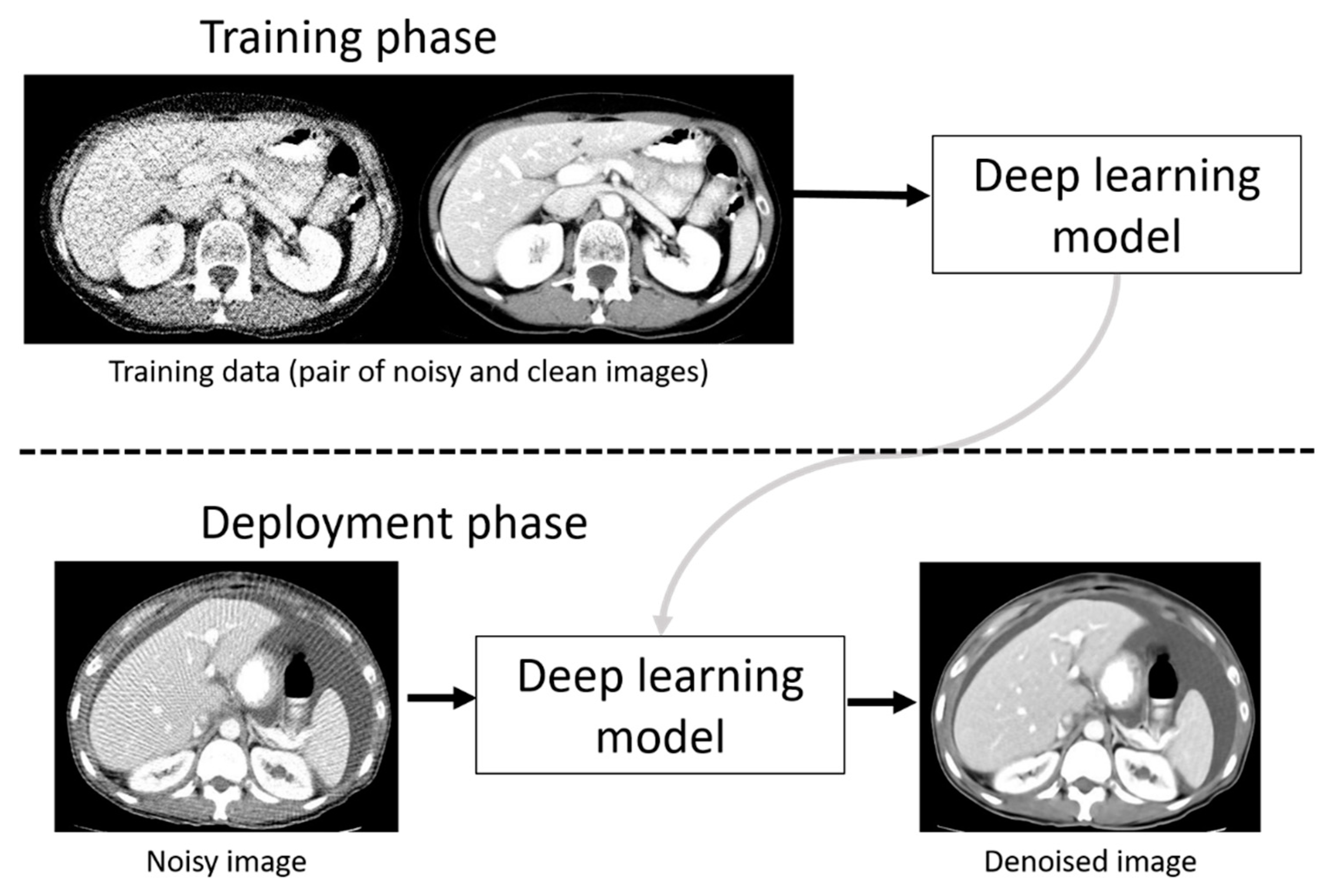
To denoise the sparse-sampling CT images, a deep learning model was employed in the current study. The outline of the training phase and deployment (denoising) phase using a deep learning model is represented in Figure 1. In the training phase, pairs of original and noisy CT images were used for constructing a deep learning model. In the deployment phase, we used the deep learning model for denoising noisy CT images. We used a workstation with GPU (GeForce RTX 2080 Ti with 11 GB memory, NVIDIA Corporation, Santa Clara, California, USA) for training and denoising.

Two types of deep learning models were evaluated: Residual Encoder-Decoder Convolutional Neural Network (RED-CNN) [7] and deeper U-net with skip connection [6]. RED-CNN combines autoencoder, deconvolution network, and shortcut connections into its network structure, and it performed well in denoising low-dose CT images. RED-CNN used image patches extracted from the CT image (size 55 × 55 pixels) for training [7]. Nakai et al. developed deeper U-net for denoising sparse-sampling chest CT images and showed that deeper U-net was superior to conventional U-net with skip connection [6]. Contrary to RED-CNN, deeper U-net made it possible to use entire CT images (size 512 × 512 pixels) as training data. In the current study, the usefulness of deeper U-net was evaluated and compared to RED-CNN.

We implemented deeper U-net using Keras (version 2.2.2, https://keras.io/) with TensorFlow (version 1.10.1, https://www.tensorflow.org/) backend. The major differences of network structure between our deeper U-net and Nakai’s deeper U-net were as follows: (i) the number of maxpooling and upsampling was 9; (ii) the numbers of feature maps in the first convolution layer of our U-net was 104. After the maxpooling layer, the number of feature maps in the convolution layer was doubled. However, if the numbers of feature maps were 832, the number of feature maps was not increased even after the maxpooling layer. The changes in the network structure of our deeper U-net including (i) and (ii) are shown in Appendix A in more detail. To train deeper U-net, pairs of original CT images and sparse-sampling CT images were prepared. Mean squared error (MSE) between the original and denoised CT images represented the loss function of deeper U-net. Adam was used as an optimizer, and its learning rate was 0.0001. The number of training epochs was 100. 4000 seconds were required for training deeper U-net per one epoch.

RED-CNN was trained using its PyTorch implementation (https://github.com/SSinyu/RED_CNN). RED-CNN was trained on an image patch size of 55 × 55 pixels. Network-related parameters of RED-CNN were retained as described previously [7].

2.4. Quantitative Image Analysis

To evaluate the denoising performance of deep learning models, we used two quantitative measures, PSNR and SSIM, on the 4667 CT images from 50 test cases [23]. These parameters are frequently used as standard objective distortion measures and for quantitative assessment of the reconstructed images [10]. PSNR is defined as

$$PSNR=20{log}_{10}(\frac{MA{X}_I}{\sqrt{MSE}}),$$

(1)

where MSE is calculated between the denoised and original CT images, and MAX_I is the maximum value of the original CT image. SSIM is a metric that supposedly reflects the human visual perception rather than PSNR. It is defined as

$$SSIM(x,y)=\frac{(2u_x{u}_y+c_1)(2s_{xy}+c_2)}{(u_x^2+u_y^2+c_1)(s_{x2}+s_{y2}+c_2)},$$

(2)

where x and y are the denoised and original CT images, respectively; u_x and u_y are the means of x and y, respectively; s_x2 and s_y2 are the variances of x and y, respectively; s_xy is the covariance of x and y; and c₁ and c₂ are determined by the dynamic range of the pixel values to stabilize the division with the weak denominator. Scikit-image (version 0.13.0, https://scikit-image.org/) was used to calculate these two quantitative measures.

2.5. Qualitative Image Analysis

On the denoised sparse-sampling CT of 50 test cases, the normal and abnormal lesions were visually evaluated. For the qualitative evaluation, four radiologists were participated, two performing visual assessments as readers and the other two defining and extracting lesions to be assessed. The two groups were independent of each other.

As readers, two board-certified radiologists (with 17 and 10 years of experience, respectively) independently evaluated the denoised CT images and referred to the original images on 3D Slicer (version 4.10.2, https://www.slicer.org/) [24]. For all visual evaluations described in the following section, we used a five-point scale as follows: (1) Unacceptable, (2) Poor, (3) Moderate, (4) Good, and (5) Excellent. The definition of each score and detail procedure of qualitative evaluation is shown in

Table 1. Score criteria for entire CT image quality.

(A) Overall Image Quality
Score
1	Unacceptable	non-diagnostic
2	Poor	poor visualization, heavily blurred appearance of structures
3	Moderate	moderate visualization, moderate blurring
4	Good	good delineation, slight blurring
5	Excellent	excellent visualization, sharp delineation (equivalent to or better compared with the original image)
(B) Noise and Artifacts
Score
1	Unacceptable	heavily noise and artifacts, structures are not visible on entire CT image
2	Poor	heavily noise and artifacts, structures are not visible on most parts of CT image
3	Moderate	moderate noise and artifacts, but acceptable for clinical evaluation
4	Good	minor, but slight noticeable noise and artifacts are found compared with the original image
5	Excellent	noise and artifacts levels are equivalent to or better compared with the original image

,

Table 2. Score criteria for the evaluation of normal local lesions (common iliac artery, internal iliac artery, and external iliac artery).

Score
1	Unacceptable	Unrecognizable
2	Poor	recognizable, but not measurable
3	Moderate	recognizable and measurable despite a blurred margin
4	Good	slightly blurry margin compared with the original image, but measurable
5	Excellent	measurable, sharp margin equivalent to the original image

and

Table 3. Score criteria for the evaluation of abnormal lesions.

Score
1	Unacceptable	unrecognizable
2	Poor	recognizable but unqualified for diagnosis and measurement
3	Moderate	moderately noisy and blurry, but recognizable and qualified for diagnosis and measurement
4	Good	qualified for diagnosis and measurement, but slightly inferior to the original image
5	Excellent	qualified for diagnosis and measurement equivalent to the original image

and Appendix B, respectively.

The image quality evaluation of the entire CT and the normal local lesions were evaluated. For the entire CT image quality, (A) Overall image quality and (B) Noise and artifacts were evaluated. The overall image quality represented a comprehensive evaluation, including noise, artifacts, and visibility of anatomical structures.

As an evaluation of the normal local lesions, the visibility of the iliac artery (the common iliac artery, internal iliac artery, and external iliac artery) was evaluated. A score was given on whether or not the diameter could be reliably measured at each of the three points of the common iliac artery, internal iliac artery, and external iliac artery.

Peritoneal dissemination, liver metastasis, and lymph node metastasis were visually evaluated as abnormal lesions by the two radiologists. The abnormal lesions were determined by the consensus of two other independent board-certified radiologists (6 and 14 years of experience, respectively) on the original CT image based on the following criteria. Peritoneal dissemination was defined as previously established as either 1) an isolated mass or 2) subtle soft tissue infiltration and reticulonodular lesions [25]. Lymph node metastasis was defined as short axis ≥10 mm. With reference to RESIST v1.1, we defined peritoneal dissemination and liver metastasis as follows: peritoneal dissemination for non-measurable or measurable (long axis ≥ 10 mm); liver metastasis (long axis ≥ 10 mm) [26]. The measurable lesions of peritoneal dissemination were further subdivided into long axis ≤ 20 and > 20 mm because the staging of FIGO 2014 differs depending on the size [27].

2.6. Statistical Analysis

For the quantitative assessment of the denoised images, the mean scores of PSNR and SSIM of deeper U-net and RED-CNN were calculated. All the qualitative image quality scores were compared between deeper U-net and RED-CNN using the Wilcoxon signed-rank test. For each abnormal lesion, a 5-point score ≥ 3 was regarded as true positive (TP), and a 5-point score < 3 as false negative (FN). He detectability of abnormal lesions was calculated based on the following equation: $\frac{TP}{TP+FN}$ (sensitivity). The detectability of abnormal lesions was compared between deeper U-net and RED-CNN using the McNemar test. Statistical analyses were performed using JMP^® (version 14.2, SAS Institute Inc., Cary, NC, USA). All tests were two sided with a significance level of 0.05.

3. Results

A summary of patient demographics of the 141 cases is provided in

Table 4. Patient demographics of TCGA-OV.

Category		Value
Age *		60.7 ± 11.2 (39–82)
Location of tumor
	Bilateral	107
	Left	13
	Right	12
	Not available	8
Clinical Stage **
	IB	1
	IC	7
	IIA	3
	IIB	1
	IIC	4
	IIIA	1
	IIIB	3
	IIIC	93
	IV	26
	Not available	1

Note: * and ** indicate that data were obtained from 139 and 140 cases, respectively. Clinical stage of patients were extracted from the TCGA-OV dataset; it is unknown whether the clinical stage is based on FIGO classification or TNM classification.

. The location of ovarian cancer and clinical stage were available from TCIA in 140 cases. Age was obtained from DICOM data of CT images. For the 50 test cases, 124 abnormal lesions were determined, including 6 liver metastases, 25 lymph node metastases, and 93 peritoneal disseminations. For the peritoneal disseminations, the numbers of non-measurable lesions, measurable lesions with long axis ≤ 20 mm, and measurable lesions with long axis > 20 mm were 53, 28, and 12, respectively.

For normal local lesions and abnormal lesions, representative images of the original CT and denoised CT obtained using deeper U-net and RED-CNN are shown in Figure 2. Additionally, representative images of the original CT, the sparse-sampled CT images before denoised processing and denoised CT obtained using deeper U-net and RED-CNN are shown in Figure 3.

3.1. Quantitative Image Analysis

We evaluate the PSNR and SSIM on the 4667 CT images from 50 test cases. The number of samples for calculating PSNR and SSIM was 4667. The PSNR and SSIM were 29.2 ± 1.49 and 0.75 ± 0.04 for the sparse-sampling images before denoising, 48.5 ± 2.69 and 0.99 ± 0.01 for deeper U-net, and 37.3 ± 1.97 and 0.93 ± 0.02 for RED-CNN.

3.2. Qualitative Image Analysis

The results of the visual evaluation are shown in Figure 4 and Figure 5 and

Table 5. Visual evaluation of entire CT image quality by the two readers using different deep learning algorithms.

(A) Overall Image Quality
Reader 1			Reader 2
score	Deeper U-net	RED-CNN	score	Deeper U-net	RED-CNN
1	1	41	1	2	42
2	5	7	2	0	8
3	24	2	3	22	0
4	20	0	4	26	0
5	0	0	5	0	0
(B) Noise and Artifacts
Reader 1			Reader 2
score	Deeper U-net	RED-CNN	score	Deeper U-net	RED-CNN
1	1	41	1	1	43
2	7	8	2	3	7
3	20	1	3	5	0
4	21	0	4	39	0
5	1	0	5	2	0

and

Table 6. Visual evaluation of normal local lesions and abnormal lesions by the two readers using different deep learning algorithms.

(A) Normal Local Lesions
Reader 1			Reader 2
score	Deeper U-net	RED-CNN	score	Deeper U-net	RED-CNN
1	0	2	1	0	0
2	1	21	2	3	42
3	7	21	3	6	8
4	12	6	4	31	0
5	30	0	5	10	0
(B) Abnormal Lesions
Reader 1			Reader 2
score	Deeper U-net	RED-CNN	score	Deeper U-net	RED-CNN
1	2	16	1	13	0
2	6	30	2	66	5
3	26	69	3	44	35
4	56	9	4	0	68
5	34	0	5	0	15

. For all items of the visual evaluation, deeper U-net scored better than that of RED-CNN for both readers as shown in

Table 7. Results of visual evaluations by the two readers using different deep learning algorithms.

		Deeper U-net	RED-CNN	p
Entire CT image quality
(A) Overall image quality	Reader 1	median, 3; IQR, 3 to 4	median, 1; IQR, 1 to 1	<0.0001
	Reader 2	median, 4; IQR, 3 to 4	median, 1; IQR, 1 to 1	<0.0001
(B) Noise and artifacts	Reader 1	median, 3; IQR, 3 to 4	median, 1; IQR, 1 to 1	<0.0001
	Reader 2	median, 4; IQR, 4 to 4	median, 1; IQR, 1 to 1	<0.0001
Normal local lesions	Reader 1	median, 5; IQR, 4 to 5	median, 3; IQR, 2 to 3	<0.0001
	Reader 2	median, 4; IQR, 4 to 4	median, 2; IQR, 2 to 2	<0.0001
Abnormal lesions	Reader 1	median, 4; IQR, 3 to 5	median, 3; IQR, 2 to 3	<0.0001
	Reader 2	median, 4; IQR, 3 to 4	median, 2; IQR, 2 to 3	<0.0001

Abbreviation: IQR, interquartile range; RED-CNN, Residual Encoder-Decoder Convolutional Neural Network.

.

Streak artifacts tended to be stronger on images at the upper abdomen level, especially where the lung and abdominal organs were visualized on the same image.

The detectability of abnormal lesions with deeper U-net was significantly better than that with RED-CNN: 95.2% (118/124) vs. 62.9% (78/124) (p < 0.0001) for reader 1 and 97.6% (121/124) vs. 36.3% (45/124) (p < 0.0001) for reader 2. The number of FN with deeper U-net were six and three for readers 1 and 2, respectively. All these abnormal lesions were non-measurable peritoneal dissemination, which were identified as slight subtle soft-tissue infiltration and reticulonodular lesions on the original CT image. The representative images of the FN case are shown in Figure 6.

4. Discussion

In the current study, we compared the quantitative and qualitative image quality of sparse-sampling CT denoised with deeper U-net and RED-CNN. RED-CNN was compared with our deeper U-net because of its similar network structure [7]. For quantitative analysis, mean scores of PSNR and SSIM of CT image quality with deeper U-net were better than those with RED-CNN. For all of the visual evaluation items, the scores of CT image quality with deeper U-net were significantly better than those of RED-CNN. In addition, the detectability of ovarian cancer metastasis was more than 95% in deeper U-net.

A few studies on deep learning-based reconstruction have shown that it improved image quality and reduced noise and artifacts better than hybrid IR and MBIR [8,16,28]. Nakamura et al. reported that deep learning reconstruction could reduce noise and artifacts more than hybrid IR could and that it may improve the detection of low-contrast lesions when evaluating hypovascular hepatic metastases [16]. While their study did not evaluate low-dose CT, the deep learning model is also considered an effective method with the potential to use lower-dose CT techniques such as sparse sampling with clinically acceptable results [5]. Our results showed that denoising with deeper U-net could be used to detect ovarian cancer metastasis.

To the best of our knowledge, this was the first study that evaluated the detectability of cancer metastasis, including peritoneal dissemination, liver metastasis, and lymph node metastasis on deep learning-based reconstructed CT images. The usefulness of sparse-sampling CT with deep learning has been previously reported [6,7,9,10], but image evaluation was limited to quantitative measures in most of these studies. While Nakai et al. reported on quantitative and qualitative assessments of the efficacy of deep learning on chest CT images [6], our study evaluated the usefulness of sparse-sampling CT denoised with deep learning techniques from the clinical viewpoint. We have proven that deeper U-net has an excellent ability to improve image quality and detectability of metastasis, and it could prove effective in clinical practice.

The performance difference between deeper U-net and RED-CNN was significant when assessing sparse-sampling CT images. A strong streak artifact around bony structures affected the image quality of sparse-sampling CT [29]. Therefore, to improve the image quality of sparse-sampling CT, an ideal deep learning model should reduce streak artifact associated with anatomical structures. RED-CNN used an image patch (size 55 × 55 pixels) for its training, therefore the algorithm had difficulty discerning between a streak artifact and anatomical structures. As a result, reducing the streak artifact related to anatomical structure may be limited in RED-CNN. In contrast, since deeper U-net used the entire CT image (size 512 × 512 pixels) for training, deeper U-net could be optimized to reduce streak artifact related to anatomical structures. This difference between the two deep learning models may lead to performance differences shown in the current study.

Since score 5 was defined as image quality and visualization equivalent to original CT (Table 1, Table 2 and Table 3), the denoised CT images of deeper U-net was not the same image quality as original CT images from the viewpoint of score. However, the visual scores and detectability of deeper U-net were sufficiently high.

Although patients with peritoneal dissemination are diagnosed as advanced stage, complete debulking surgery can be expected to improve the prognosis in epithelial malignant ovarian tumor [30]. In addition, there are some histological types with a favorable prognosis due to successful chemotherapy, such as yolk sac tumor [31]. Thus, the reduction of CT-radiation exposure is essential for patients with ovarian cancer. With our proposed method, theoretically, the CT radiation exposure can be reduced to one-tenth of that of the original CT. The reduction of radiation exposure may reduce the incidence of radiation-induced cancer. Furthermore, while we evaluated about only the detection of metastasis of malignant ovarian tumors in the current study, we speculate that the proposed method may be applied to other diseases.

While our results show that deeper U-net proved useful in detecting cancer metastasis, there were several drawbacks in the model. First, fine anatomical structures were obscured due to excessive denoising. This effect might be minimized by blending images of FBP and deep learning-based reconstruction, such as hybrid IR and MBIR, by adjusting radiation exposure (rate of sparse sampling) and blending rate. Secondly, the strong streak artifacts around the prosthesis and the upper abdomen compromised diagnostic ability near these anatomical lesions. Furthermore, streak artifacts tended to be stronger on images at the upper abdomen level, especially where the lung and abdominal organs were visualized on the same image. This effect may have resulted from the relatively small number of training data images that included both lung and abdominal organs compared to images that included only abdominal organs. Since ovarian cancer primarily metastasizes to the peritoneal liver surface and the liver, improving the image quality in these areas is considered a future research area. Increasing the number of training data images with cross-sections displaying both the lung and abdominal organs may help improve image quality and reduce streak artifacts in deep learning models, including deeper U-net.

Our study had several limitations. First, we used images from only one public database. The application of our deep learning model should be further evaluated in other databases. Second, sparse-sampling images cannot be obtained from real CT scanners at the current time. Our simulated subsampled images may differ from the images on real scanners. In future, we need to evaluate the performance of our deeper U-net using real CT acquisitions. Third, images obtained with the deep learning model of GAN tended to be more “natural” than those obtained with conventional deep learning model. However, the noise reduction of GAN is weaker than that of a conventional deep learning model [17]. There was a concern that the radiologist’s ability to detect metastasis might decline if the noise reduction was insufficient. Therefore, GAN was not used in the current study. Finally, because of our study design, we did not evaluate false positives, true negatives, and specificity in the current study. Therefore, it is necessary to conduct radiologists’ observer studies in which false positives and true negatives are evaluated.

5. Conclusions

Sparse-sampling CT with deep learning reconstruction could prove useful in detecting metastasis of malignant ovarian tumors and might contribute to reducing CT radiation exposure. With our proposed method, theoretically, the CT radiation exposure can be reduced to one-tenth of that of the original CT, while keeping the detectability of ovarian cancer metastasis more than 95%. It may reduce the incidence of radiation-induced cancer.

References

1. Ferlay, J.; Colombet, M.; Soerjomataram, I.; Mathers, C.; Parkin, D.M.; Piñeros, M.; Znaor, A.; Bray, F. Estimating the global cancer incidence and mortality in 2018: GLOBOCAN sources and methods. Int. J. Cancer 2019, 144, 1941–1953. [Google Scholar] [CrossRef] [Green Version]
2. Heints, A.; Odicino, F.; Maisonneuve, P.; Qiomm, M.A.; Benedet, J.L.; Creasman, W.T.; Ngan, H.Y.S.; Pecorelli, S.; Beller, U. Carcinoma of the ovary. Int. J. Gynecol. Obstet. 2006, 95, s161–s192. [Google Scholar] [CrossRef]
3. Webb, P.M.; Jordan, S.J. Epidemiology of epithelial ovarian cancer. Best Pract. Res. Clin. Obstet. Gynaecol. 2017, 41, 3–14. [Google Scholar] [CrossRef] [Green Version]
4. Shao, Y.-H.; Tsai, K.; Kim, S.; Wu, Y.-J.; Demissie, K. Exposure to Tomographic Scans and Cancer Risks. JNCI Cancer Spectr. 2019, 4, pkz072. [Google Scholar] [CrossRef] [PubMed]
5. Willemink, M.J.; Noël, P.B. The evolution of image reconstruction for CT—From filtered back projection to artificial intelligence. Eur. Radiol. 2019, 29, 2185–2195. [Google Scholar] [CrossRef] [PubMed] [Green Version]
6. Nakai, H.; Nishio, M.; Yamashita, R.; Ono, A.; Nakao, K.K.; Fujimoto, K.; Togashi, K. Quantitative and Qualitative Evaluation of Convolutional Neural Networks with a Deeper U-Net for Sparse-View Computed Tomography Reconstruction. Acad. Radiol. 2019, 27, 563–574. [Google Scholar] [CrossRef] [PubMed]
7. Chen, H.; Zhang, Y.; Kalra, M.K.; Lin, F.; Chen, Y.; Liao, P.; Member, S.; Wang, G. Low-Dose CT with a Residual Encoder-Decoder Convolutional Neural Network (RED-CNN). IEEE Trans. Med. Imaging 2017, 36, 2524–2534. [Google Scholar] [CrossRef]
8. Tatsugami, F.; Higaki, T.; Nakamura, Y.; Yu, Z.; Zhou, J.; Lu, Y.; Fujioka, C.; Kitagawa, T.; Kihara, Y.; Iida, M.; et al. Deep learning–based image restoration algorithm for coronary CT angiography. Eur. Radiol. 2019, 29, 5322–5329. [Google Scholar] [CrossRef]
9. Jin, K.H.; McCann, M.T.; Froustey, E.; Unser, M. Deep Convolutional Neural Network for Inverse Problems in Imaging. IEEE Trans. Image Process. 2017, 26, 4509–4522. [Google Scholar] [CrossRef] [Green Version]
10. Han, Y.; Ye, J.C. Framing U-Net via Deep Convolutional Framelets: Application to Sparse-View CT. IEEE Trans. Med. Imaging 2018, 37, 1418–1429. [Google Scholar] [CrossRef] [Green Version]
11. Nishio, M.; Nagashima, C.; Hirabayashi, S.; Ohnishi, A.; Sasaki, K.; Sagawa, T.; Hamada, M.; Yamashita, T. Convolutional auto-encoders for image denoising of ultra-low-dose CT. Heliyon 2017, 3, e00393. [Google Scholar] [CrossRef] [Green Version]
12. Kang, E.; Koo, H.J.; Yang, D.H.; Seo, J.B.; Ye, J.C. Cycle-consistent adversarial denoising network for multiphase coronary CT angiography. Med. Phys. 2019, 46, 550–562. [Google Scholar] [CrossRef]
13. Wolterink, J.M.; Leiner, T.; Viergever, M.A.; Išgum, I. Generative adversarial networks for noise reduction in low-dose CT. IEEE Trans. Med. Imaging 2017, 36, 2536–2545. [Google Scholar] [CrossRef] [PubMed]
14. Kang, E.; Min, J.; Ye, J.C. A deep convolutional neural network using directional wavelets for low-dose X-ray CT reconstruction. Med. Phys. 2017, 44, e360–e375. [Google Scholar] [CrossRef] [Green Version]
15. Mookiah, M.R.K.; Subburaj, K.; Mei, K.; Kopp, F.K.; Kaesmacher, J.; Jungmann, P.M.; Foehr, P.; Noel, P.B.; Kirschke, J.S.; Baum, T. Multidetector Computed Tomography Imaging: Effect of Sparse Sampling and Iterative Reconstruction on Trabecular Bone Microstructure. J. Comput. Assist. Tomogr. 2018, 42, 441–447. [Google Scholar] [CrossRef] [PubMed]
16. Nakamura, Y.; Higaki, T.; Tatsugami, F.; Zhou, J.; Yu, Z.; Akino, N.; Ito, Y.; Iida, M.; Awai, K. Deep Learning–based CT Image Reconstruction: Initial Evaluation Targeting Hypovascular Hepatic Metastases. Radiol. Artif. Intell. 2019, 1, e180011. [Google Scholar] [CrossRef]
17. Blau, Y.; Michaeli, T.; Israel, T. The Perception-Distortion Tradeoff Yochai. Proc. IEEE Conf. Comput. Vis. Pattern Recognit. 2018, 6228–6237. [Google Scholar] [CrossRef] [Green Version]
18. Clark, K.; Vendt, B.; Smith, K.; Freymann, J.; Kirby, J.; Koppel, P.; Moore, S.; Phillips, S.; Maffitt, D.; Pringle, M.; et al. The cancer imaging archive (TCIA): Maintaining and operating a public information repository. J. Digit. Imaging 2013, 26, 1045–1057. [Google Scholar] [CrossRef] [Green Version]
19. TCGA-OV. Available online: http://doi.org/10.7937/K9/TCIA.2016.NDO1MDFQ (accessed on 20 December 2019).
20. TCGA Attribution. Available online: http://cancergenome.nih.gov/ (accessed on 20 December 2019).
21. Van Aarle, W.; Palenstijn, W.J.; Cant, J.; Janssens, E.; Bleichrodt, F.; Dabravolski, A.; De Beenhouwer, J.; Joost Batenburg, K.; Sijbers, J. Fast and flexible X-ray tomography using the ASTRA toolbox. Opt. Express 2016, 24, 25129. [Google Scholar] [CrossRef]
22. Van Aarle, W.; Palenstijn, W.J.; De Beenhouwer, J.; Altantzis, T.; Bals, S.; Batenburg, K.J.; Sijbers, J. The ASTRA Toolbox: A platform for advanced algorithm development in electron tomography. Ultramicroscopy 2015, 157, 35–47. [Google Scholar] [CrossRef] [Green Version]
23. Wang, Z.; Bovik, C.; Sheikh, H.R.; Simoncelli, E.P. Image Quality Assessment: From Error Visibility to Structural Similarity. IEEE Trans. Image Process. 2004, 13, 600–612. [Google Scholar] [CrossRef] [PubMed] [Green Version]
24. Fedorov, A.; Beichel, R.; Kalpathy-Cramer, J.; Finet, J.; Fillion-Robin, J.-C.; Pujol, S.; Jennings, D.; Bauer, C.; Sonka, M.; Fennessy, F. 3D Slicer as an Image Computing Platform for the Quantitative Imaging Network. Magn. Reson. Imaging 2012, 30, 1323–1341. [Google Scholar] [CrossRef] [Green Version]
25. Nougaret, S.; Addley, H.C.; Colombo, P.E.; Fujii, S.; Al Sharif, S.S.; Tirumani, S.H.; Jardon, K.; Sala, E.; Reinhold, C. Ovarian carcinomatosis: How the radiologist can help plan the surgical approach. Radiographics 2012, 32, 1775–1800. [Google Scholar] [CrossRef] [PubMed] [Green Version]
26. Eisenhauer, E.A.; Therasse, P.; Bogaerts, J.; Schwartz, L.H.; Sargent, D.; Ford, R.; Dancey, J.; Arbuck, S.; Gwyther, S.; Mooney, M.; et al. New response evaluation criteria in solid tumours: Revised RECIST guideline (version 1.1). Eur. J. Cancer 2009, 45, 228–247. [Google Scholar] [CrossRef] [PubMed]
27. Mutch, D.G.; Prat, J. 2014 FIGO staging for ovarian, fallopian tube and peritoneal cancer. Gynecol. Oncol. 2014, 133, 401–404. [Google Scholar] [CrossRef]
28. Akagi, M.; Nakamura, Y.; Higaki, T.; Narita, K.; Honda, Y.; Zhou, J.; Yu, Z.; Akino, N.; Awai, K. Deep learning reconstruction improves image quality of abdominal ultra-high-resolution CT. Eur. Radiol. 2019, 29, 6163–6171. [Google Scholar] [CrossRef]
29. Jin, S.O.; Kim, J.G.; Lee, S.Y.; Kwon, O.K. Bone-induced streak artifact suppression in sparse-view CT image reconstruction. Biomed. Eng. Online 2012, 11, 1–13. [Google Scholar] [CrossRef] [Green Version]
30. Du Bois, A.; Reuss, A.; Pujade-Lauraine, E.; Harter, P.; Ray-Coquard, I.; Pfisterer, J. Role of surgical outcome as prognostic factor in advanced epithelial ovarian cancer: A combined exploratory analysis of 3 prospectively randomized phase 3 multicenter trials: By the arbeitsgemeinschaft gynaekologische onkologie studiengruppe ovarialkarzin. Cancer 2009, 115, 1234–1244. [Google Scholar] [CrossRef]
31. Faure Conter, C.; Xia, C.; Gershenson, D.; Hurteau, J.; Covens, A.; Pashankar, F.; Krailo, M.; Billmire, D.; Patte, C.; Fresneau, B.; et al. Ovarian yolk sac tumors; does age matter? Int. J. Gynecol. Cancer 2018, 28, 77–84. [Google Scholar] [CrossRef]
Figure 1. Outline of the training phase and deployment phase of the deep learning model.
Applsci 10 04446 g001
Figure 2. Representative images of the original CT and denoised CT obtained using deeper U-net and RED-CNN. Note: (A) Visual scores of common iliac artery (red arrow): 5 points for deeper U-net, 2 points for RED-CNN for reader 1; 4 points for deeper U-net, 2 points for RED-CNN for reader 2. (B) Visual scores of liver metastasis (yellow arrow): 3 points for deeper U-net, 2 points for RED-CNN for reader 1; 4 points for deeper U-net, 2 points for RED-CNN for reader 2. Abbreviation: RED-CNN, Residual Encoder-Decoder Convolutional Neural Network.
Applsci 10 04446 g002
Figure 3. Representative images of the original CT, sparse-sampling CT before denoising, and denoised CT obtained using deeper U-net and RED-CNN. Note: (A) Case 1: Visual scores of peritoneal dissemination (white circle): 4 points for deeper U-net, 1 points for RED-CNN for reader 1; 4 points for deeper U-net, 1 points for RED-CNN for reader 2. (B) Case 2: Visual scores of lymph node metastasis (yellow arrow): 5 points for deeper U-net, 2 points for RED-CNN for reader 1; 4 points for deeper U-net, 2 points for RED-CNN for reader 2. (C) Case 3: Visual scores of liver metastasis (red arrow): 4 points for deeper U-net, 2 points for RED-CNN for reader 1; 4 points for deeper U-net, 2 points for RED-CNN for reader 2. (D) Case 4: Visual scores of peritoneal dissemination (red arrow): 4 points for deeper U-net, 2 points for RED-CNN for reader 1; 4 points for deeper U-net, 1 points for RED-CNN for reader 2.
Applsci 10 04446 g003aApplsci 10 04446 g003b
Figure 4. Visual evaluation of entire CT image quality by the two readers using different deep learning algorithms.
Applsci 10 04446 g004
Figure 5. Visual evaluation of normal local lesions and abnormal lesions by the two readers using different deep learning algorithms.
Applsci 10 04446 g005
Figure 6. A representative undiagnosable lesion on denoised CT image with deeper U-net. Note: The circle shows non-measurable peritoneal dissemination. With deeper U-net, the score was 1 point for reader 1 and 2 points for reader 2.
Applsci 10 04446 g006