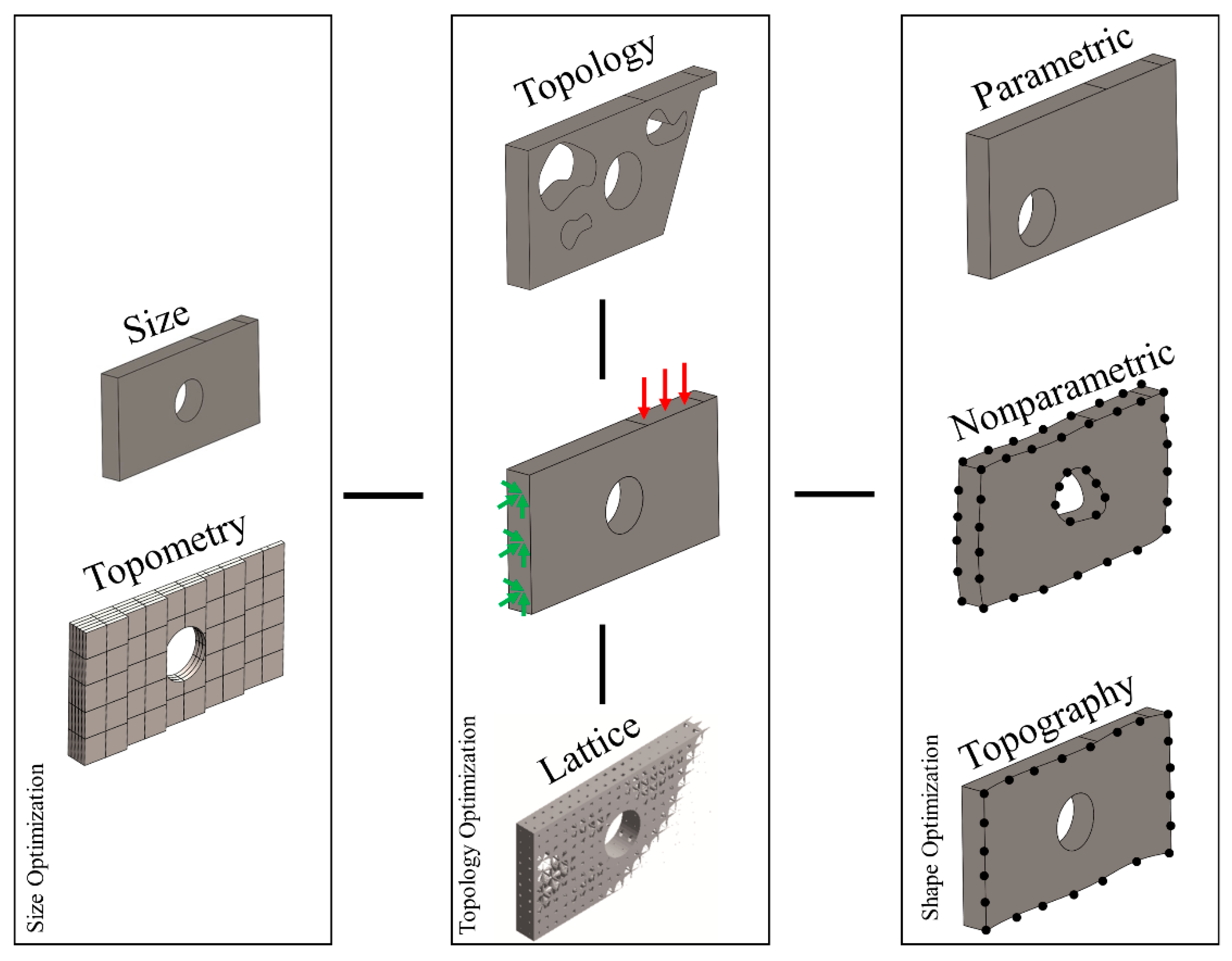
Article

Topology and Parametric Optimization-Based Design Processes for Lightweight Structures

by
Evangelos Tyflopoulos
* and
Martin Steinert
Department of Mechanical and Industrial Engineering, Norwegian University of Science and Technology (NTNU), 7491 Trondheim, Norway
*
Author to whom correspondence should be addressed.
Appl. Sci. 2020, 10(13), 4496; https://doi.org/10.3390/app10134496
Submission received: 27 May 2020 / Revised: 20 June 2020 / Accepted: 25 June 2020 / Published: 29 June 2020
(This article belongs to the Section Mechanical Engineering)

Abstract

:
Topology and Parametric Optimization are two of the most implemented material optimization approaches. However, it is not clear in the literature which optimization procedure, or possible combination of them, can lead to the best results based on material reduction and optimization time. In this paper, a quantitative comparison of different topology and parametric optimization design processes is conducted using three benchmark examples: A Hollow Plate, an L-Bracket, and a Messerschmitt–Bölkow–Blohm Beam (MBB-Beam). Ten different design processes that were developed in each case study resulted in 30 simulations in total. The design processes were clustered in three main design workflows: The Topology Optimization, the Parametric Optimization, and the Simultaneous Parametric and Topology Optimization. Their results were compared with respect to mass, stress, and time. The Simultaneous Parametric and Topology Optimization approach gave the lightest design solutions without compromising their initial strength but also increased the optimization time. The findings of this paper will help the designers in the pursuit of lightweight structures and will create the basis for the identification of the ideal material optimization procedure.

1. Introduction

Two notable categories in Structural Optimization (SO) are the Parametric Optimization (PO) and Topology Optimization (TO). These optimization approaches have been increasingly applied as material reduction methods in the industry over the last decades. The gains from these optimization methods are notable and have thoroughly been presented in the literature [1,2].
On the one hand, PO allows a selective optimization of the model based on the given parameters and their value range. It can easily guide to global shape and size optimum solutions for linear and convex problems, but it cannot optimize the topology of the structure [3]. Furthermore, both the Design of Experiments (DOE) and Sensitivity Analysis (SA) were developed simultaneously with the PO to support the implementation and the choice of the most crucial parameters in optimization, respectively [4].
On the other hand, TO reduces the material usage while enhancing both the quality and the robustness of the structures. In addition, it increases the design flexibility, as well as shortens the design process and thus the time to market [5]. However, it is a hard and time-demanding procedure, which can result in complex shapes that are difficult and expensive to be manufactured. For this reason, TO can be categorized as TO for Additive Manufacturing (AM) and TO for Conventional Manufacturing Processes (CMP). The traditional TO is mainly oriented to AM. In general, the topologically optimized design solutions are characterized by their organic shapes. AM enables the direct use of these shapes and decreases the number of geometric restrictions. However, it is possible to prefer CMP to AM. In this case, the designer adds the corresponding geometric restrictions due to manufacturing constraints, such as design for extrusion or size minimums [6]. The choice between these two different TO orientations depends on the optimized design, the cost, and the production time.
A plethora of research papers focused on either development of new approaches or improvement of the existing optimization methods [7,8]. However, there is limited literature that compares the aforementioned optimization methods or possible combinations of them with respect to their results and optimization time [9,10]. The identification of the ideal design process is challenging. Furthermore, the geometric and boundary uncertainties in a fuzzy design environment make this decision harder. In this paper, the authors answer critical questions about practical issues in both TO and PO. Concerning the post-processing of the topology optimized results, it is not clear if a designer will use them as a starting point of his/her initial designs or if they will constitute the final designs of a structure. In the second case, AM, with 3D printing, is inevitable as a manufacturing method while the CMP can mainly be used in the first case. Furthermore, possible combinations between topology and parametric optimization were explored in the pursuit of the ideal design process with respect to mass reduction and maximum stress as measuring parameters. In addition to them, an approximation of the optimization time was calculated. The optimization time encompasses the used time for the individual phases of TO, PO, Validation (V), and Redesign (R) and was calculated based on the software’s outputs and the designer’s measurements. Different combinations of topology and parametric optimization were developed. In particular, ten design processes were created in this comparative study. The main goal was to identify the ideal methodology based on the aforementioned parameters. For this reason, three benchmarking examples, a Hollow Plate, an L-Bracket, and a Messerschmitt–Bölkow–Blohm Beam (MBB-Beam), were used as case studies. The designer looking for lightweight structures could use the findings of this paper to choose the design process that fits his/her design case and optimization goals.
This paper is composed as follows: In Section 2, the different, most known types of SO are presented as well as the theoretical background of the implemented topology optimization method in this paper. The conducted experimental design process follows in Section 3. Subsequently, in Section 4, the results of the three case studies are presented and discussed, and finally, the conclusions and the future research based on the findings in this paper are presented in Section 5 and Section 6, respectively.

2. Types of Structural Optimization

Structural Optimization (SO) is a mathematical optimization of the structure’s material with respect to given boundary conditions and constraints [11]. Sigmund [12] categorized the different SO approaches, based on the mathematical form of their objective function, to Gradient-Based Topology Optimization Techniques (GTO) and Non-Gradient Topology Optimization Techniques (NGTO).
On the one hand, the former category encompasses several approaches, such as the Homogenization Approach, the Density Approach (SIMP), and the gradient-based forms of the Level Set Method (LSM), the Evolutionary Structural Optimization (ESO), the Phase-Field Methods, and the Topological Derivatives. In general, the GTO techniques utilize algorithms that are characterized by a single-point search and, thus, suffer from multimodal problems. For this reason, NGTO techniques have also developed [13].
The NGTO techniques are stochastic approaches that were created to overcome the multimodal optimization problem as well as the derivation complexities created by the GTO, especially in commercial software tools. These methods allow multiple-point searches and utilize different evolution strategies such as Genetic Algorithms, Artificial Immune Algorithms, Ant Colonies, Particle Swarms, Simulated Annealing, Harmony Search, and Differential Evolution Schemes [12]. However, some of these strategies use gradient or gradient-like information in order to improve their evolutionary search for optimal solutions. A notable example of the latter category is the Covariance matrix adaptation evolution strategy (CMA-ES) based topology optimization, using a level set expression to solve multimodal optimal design problems [13]. In this paper, the LSM in ANSYS software (2019 R2 version, ANSYS, Inc., Canonsburg, PA, USA) was used to conduct the TO simulations. The theoretical background of this method is described in Section 2.1.
The SO, as presented by Bendsøe and Sigmund [14], consists of three different types of optimization: Size, shape, and topology. According to Mortazavi and Toğan [15], size optimization refers to the physical size of the members within the structure, such as thickness, while shape optimization refers to the geometric layout (the boundary of the state equation). There is either nonparametric (free form) or parametric shape optimization. In the case of nonparametric shape optimization, the design space consists of the surface nodes (design nodes) of the finite element model. On each of the design points, a displacement vector is placed. The scalar optimization displacements along these vectors constitute the implicit parameters in this type of free form optimization.
On the other hand, the parametric shape optimization is linked to the Computer-aided design (CAD) geometry of the structure [9]. Finally, TO generates material layout concepts by changing the number and the configuration of the structure members, i.e., the number of the holes in a structure. In these three categories, we can add the topography, topometry, and lattice optimization. Topography optimization is a particular case of shape optimization where the nodes in a structure can be moved either transverse or to a given direction related to the original points using perturbation vectors [16]. Topometry optimization is a more general type of size optimization where each element can be optimized independently [16]. Finally, lattice optimization generates a lattice-optimized structure within a region of interest by including repeating cellular structures with varying thickness [17]. Figure 1 illustrates the aforementioned types of SO by presenting an example of a Hollow Plate.
In this example, the size optimization of the plate could be the optimization of its thickness or/and its section size (length and height). In the case of nonparametric shape optimization, both the external shape of the Hollow Plate and the shape of its internal members (in this case, the hole’s shape) could be optimized. The position of the hole could be considered as parametric shape optimization. The TO could contain both the external shape of the plate, its internal member shape (hole), and the creation of new internal members, i.e., new holes for the given design space. In other words, ΤO could be considered a combined size and nonparametric shape optimization with the acceptance of either creation or removal of internal members of the structure. Regarding the subcases of topography and topometry optimization, the shape of the front face of the plate and the thickness of some of its elements could be optimized, respectively. Finally, the introduction and optimization of lattice structures [17] could be evaluated by using the lattice optimization approach.
A parametrization of a structure’s geometry could allow a PO of it. In the case of a Hollow Plate, both the length, height, thickness, and position of the hole could be used as parameters in PO. This type of optimization changes both the size and the shape of the structure but not its topology and can be considered as a traditional size/shape parametric optimization. Gradient or response surface algorithms are used in order to solve the parametric optimization problem. The choice and the amount of the parameters, as well as the range of their acceptable values, can affect the identification of the optimum design and possibly lead to infeasible design solutions [9]. For example, the parameters that define the position of the hole should always be in accordance with the upper and lower limits of the plate’s length and height. In other words, the hole is not allowed to be placed outside of the given design space. A systematic way for the identification of the input parameters (factors), their allowable values (levels), dependencies, and trade-offs, as well as their impact on the parametric optimization results (sensitivity), is mainly known as DOE. Thus, the DOE is a statistical method that helps the designer to explore, understand, and optimize his/her designs by changing the range of values of the design parameters in the same set of experiments [18].

2.1. Level Set Method

In this paper, the LSM was chosen for the TO due to its effectiveness and simplicity in the post-processing [19]. In addition to that, it can be mesh-independent and does not suffer from checkerboard discontinuities [20]. Osher and Sethian [21] introduced first the mathematical background of the level set method, which was later used effectively by Wang, Wang [22] and Allaire, Jouve [19] as an alternative topology optimization technique. The Eulerian shape parametrization of a structure is represented using a Level Set function, φ(x) with the following formulation [2,20,22]:
φ ( x ) { > 0     x s o l i d ,       = 0   x     b o u n d a r y , < 0     x v o i d .
An illustration of this level set function, as well as its design domains, is depicted in Figure 2.
The topology optimization of the structures is attained by solving the Hamilton–Jacobi equation:
dφ/dt + V × |∇φ| = 0
where:
  • t: Pseudo-time
  • V: Speed function of φ(x) change
Hence, the optimization problem is formulated as:
minimize: J(u,φ) =∫Ω F(u) × H(φ) × dΩ,
s.t.: α(u,v,φ) = L(v, φ),
: u| Γd = u0, ∀ v ∊ U,
: V = ∫Ω H(φ) × dΩ ≤ Vmax
In terms of energy bilinear form α(u,v,φ), (5), (6), and (7) can be formulated as:
α(u,v,φ) = ∫Ω Eijkl × εij (u) × εkl (v) × H(φ) × dΩ,
L(v,φ) = ∫Ω p × v × H(φ) × dΩ + ∫Γ τ × v × δ(φ) × |∇φ| × dΩ
V(φ) = ∫Ω H(φ) × dΩ
where:
  • δ(x): Dirichlet function
  • F(u): Structure volume by means of a continuous auxiliary function
  • u: Displacement field in the space U
  • H(x): Heaviside function
  • v: Volume field of volume V
  • Eijkl: Elastic tensor
  • εij: Strain tensor
  • p: Displacement
  • u0: Prescribed displacement
  • L(v,φ): Linear form of the load
  • V(φ): Volume of the structure
  • τ: Boundary tractions
  • Ω: Design space
  • Γ: Partial design space
  • Γd: Partial boundary
Here, the Level Set topology optimization of the three presented examples was implemented at the Workbench ANSYS finite element analysis software.

3. The Experimental Design Process

As already mentioned in Section 1, the aim of the authors was to develop different design processes based on possible combinations of topology and size/shape parametric optimization. Thus, ten different design processes were created and executed in an Intel Core I7-7820HQ computer with 32 GB RAM. Three case studies: A Hollow Plate, an L-Bracket, and an MBB-Beam were used to test the design processes. Hence, 30 simulations were conducted in total. Their results were compared with respect to mass, optimization time, and stress. An overview of the implemented design processes is presented in Table 1.
In addition, the authors clustered the design processes to those that can lead to designs that either can be mainly produced by AM (3D printing) or both by AM and CMP. An illustration of this categorization is depicted in Figure 3. Each of these processes consists of a maximum of four optimization levels. Furthermore, the main processes were classified, based on their first optimization level, in three main design workflows; TO, PO, and simultaneous PO and TO. The goal of these workflows was the mass reduction of the structures with respect to their yield strength. The first level optimization can be followed either by a no redesign/redesign or TO procedure at the second level and possibly, with a new PO round at third and fourth level for a further mass reduction.
The most implemented design process is the topology optimization with redesign and parametric shape optimization (TO_R_PO), process (3). A representative example of this design process in the literature is the topology optimization of the leading-edge rib of an airbus A380 [23]. The general idea of the presented methodology in this example is that first, the initial design is topologically optimized. Then, it was redesigned at the second level, and finally, it was used as input in a size/shape parametric optimization. This last step contributed to TO with an additional mass reduction of the structure. Furthermore, the redesign, together with the PO, helped in overcoming possible stress concentrations at the optimized topology design and made its manufacturing feasible by the conventional processes. However, it is not clear if this process is the ideal combination of TO and PO. It seems that relative research work is missing from the literature.
For the scope of this research, both the CAD, the Finite Element Analysis (FEA), as well as the topology and parametric optimizations, were conducted in ANSYS software. Concerning the TO, the LSM was used in ANSYS Mechanical. Furthermore, the PO was implemented in ANSYS DesignXplorer and was divided into six steps: Step 1. Definition of factors and responses, Step 2. Selection of design exploration method, Step 3. Selection of DOE method, Step 4. Creation of a response surface, Step 5. Sensitivity analysis of the results, and Step 6. Design optimization. The implemented process is depicted in Figure 4.
In the first step, the designer has to parameterize the design and decide all the possible factors (inputs) and responses (outputs) that will be used in the optimization process. On the one hand, as factors in a PO of a structure could be used, its length and thickness. On the other hand, some common responses are the mass, weight, and the volume of a structure, as well as its maximum stress, deflection, and displacement. All three presented structures here share the same goals, which are the minimization of their mass and maximum stress.
The second step is about the selection of the solution of the parametric optimization problem. In this paper, the Response Surface Methodology (RSM) was applied. The RSM was firstly developed by Box and Wilson [24] to leverage the data from DOE. It is a collection of mathematical and statistical techniques that are used to optimize simultaneously different variables of an objective function and represent their dependencies graphically [18]. The term response surface is derived from the appearance of a second-order model’s plot. A common RSM is usually based on the method of steepest ascent. For example, a first-order and a second-order regression model of two factors (k = 2) can be formulated by the following polynomials [25]:
f(x) = β0 + β1 x1 + β2 x2 + ε(x)
f(x) = β0 + β1 x1 + β2 x2 + β11 x12 + β22 x22 + β12 x1 x2 + ε(x)
where:
  • f(x): Response of the model
  • x1, x2: First-order terms
  • x12, x22: Second-order terms
  • βij: Regression coefficients
  • ε(x): Model error
The response surface plots for the two models are illustrated in Figure 5.
There are many different methods of DOE that have been developed to fit response surfaces. Some of the most known DOE methods are the Full factorial, the Fractional factorial, the Box-Behnken, the Plackett-Burman, the Latin Hypercube Sampling (LHS), the Central composite, and the Taguchi designs [18]. The selected DOE method in this paper is the LHS. The LHS is a statistical method that is used to generate random samples based on the given factors [26]. This method was preferred due to its data accuracy, efficiency, and flexibility in the presence of a large number of parameters [26]. As was presented by McKay, Beckman [27], at the LHS, the sample values are placed in a square grid, also known under the name Latin square. Unlike random sampling, the researcher using LHS needs to decide on the number and the placement of the sample points inside the square. If an experimental design consists of p design points and k number of factors (random variables), its sampling space is a p × k matrix. Each column of this matrix represents a variable, and each row a sample. An example of an LHS with two factors, nine design points, and nine levels in each factor is depicted in Figure 6. One challenge of the LHS is to place the chosen design points evenly within the design space in order to cover as much space as possible.
The next step is about the creation of a response surface for prediction purposes, based on the results from the DOE. The Polynomial, the Kriging, the Support Vector, the Feedforward neural network, and the Sparse Grid are some of the methods that can be used for the regression analysis. In this research, the Kriging method was applied. Kriging is a Gaussian regression process that is dependent on all raw data and fits automatically through all the existing points [28]. A general form of the Kriging model is the following:
y(x) = f(x) + Z(x) + ε(x)
The Z(x) is the Gaussian process and the term that differentiates the Kriging method from the polynomial regression model. Thus, the Kriging model interpolates the sampled design points and quantifies their interpolation errors.
In the fifth step, the designer can conduct a sensitivity analysis of the results. A sensitivity analysis is the calculation of the objective function uncertainties in possible factors fluctuations. This analysis can be used as a diagnostic tool by the designer and can help him/her to identify and screen the most crucial parameters among them. These parameters, in their turn, can be used as a new focus in the PO of the structure [29]. An example of a sensitivity analysis diagram is shown in Figure 7. This diagram presents the norm of the partial derivatives of the chosen objective, in this case, the mass, with respect to the selected variables, herein: Length, radius, height, and thickness.
Finally, the created prediction models can be used for design optimization. At this point, Pareto fronts can be developed for multi-objective optimization of the structures. In Pareto optimality, the plot (surface) of the objective functions, whose non-dominated vectors compose the Pareto optimal set, is called Pareto front [30]. Pareto fronts help the designer identify useful trade-offs and potential solutions among the used objective functions in PO. The most used algorithms in solving multi-objective optimization problems are Screening, Genetic, Nonlinear Programming, and Adaptive Optimization. The Multi-Objective Genetic Algorithm (MOGA), as was presented by Murata and Ishibuchi [31], was used to optimize the three structures in this paper. The mass and the maximum stress of the structures were used as an objective function and constraint, respectively in the creation of the Pareto fronts.

4. Results

As it has been already mentioned in Section 1, a Hollow Plate, an L-Bracket, and an MBB-Beam were used as case studies in this research. The presented procedure here is based on the Hollow Plate example. Identical procedures were used for the other two models. Finally, the results of all three cases are presented and discussed.

4.1. Hollow Plate

The Hollow Plate was designed at the DesignModeler, ANSYS software. The initial design of the model, as well as its boundary conditions, are depicted in Figure 8. Concerning the FEA of the component, the plate is fixed on its left side, and a vertical force F = 2000 N is applied to a specific area (denoted with force area (FA)) on the top of the plate. The model was discretized with 1 mm tetrahedrons. In addition, mesh control was used around the hole area. A structural ASTM (American Society for Testing and Materials) A36 steel was assigned to the 3D-model with the following properties: E = 200,000 MPa, ν = 0.3, ρ = 7.85 g/cm3, yield strength of 250 MPa, and ultimate strength of 460 MPa. The initial mass of the Hollow Plate was 1103.5 g. The design parameters (factors) and their allowable value range that were used in the size/shape parametric optimizations are presented in Table 2.
The optimization procedure was presented in Figure 3 and consisted of three main design workflows: Topology Optimization (TO), Parametric Optimization (PO), and Simultaneous PO and TO.

4.1.1. Topology Optimization of a Hollow Plate

This is the most common design workflow. The general idea is to identify an optimized layout through TO and then use it as a design base for further optimization with a size optimization. Firstly, the initial design of the Hollow Plate was topologically optimized using the LSM. The objective function of the optimization was the compliance of the structure, and the response constraint the minimization of its mass in a percentage. The area where the boundary conditions were applied, as well as the plate’s hole, were excluded from the optimization region (frozen area). The maximum identified mass reduction of the Hollow Plate, for a factor of safety (FOS) equal with two, was 59.82%. The optimized design was either validated as it is, redesigned and validated, or further optimized with a PO. The conducted design processes here are the (1) topology optimization with no redesign (TO_NR), (2) topology optimization with redesign (TO_R), and (3) topology optimization with redesign and parametric shape optimization (TO_R_PO). The authors used the following rule concerning the maximum of the von Mises stress, σmax ≤ 125 MPa, which corresponds to a FOS ≥ 2 (Von Mises factor of safety). Many iterations were applied to processes (1) and (2), from the TO to the validation study, etc., in order to stick to this stress rule. Concerning the size optimization in process (3), the LHS was applied as the DOE method with 50 samples. The Kriging method and the MOGA were used for the creation of the response surface and the Pareto fronts, respectively. The final designs of the aforementioned processes are depicted in Figure 9.
Concerning process (3), the design taken from process (2) was parametrized. At this level, a parametric shape optimization was conducted using small changes in the chosen factors (thicknesses and radiuses) with the procedure described in Section 4.1.2.

4.1.2. Parametric Optimization of a Hollow Plate

At this design workflow, a PO of the Hollow Plate was conducted at the first level before the TO, which now was implemented at the second level. In other words, a size/shape PO was carried out before the procedure presented in Section 4.1.1. The intention was to decrease the design space for the TO. The processes presented here are (4) parametric size/shape optimization (PO), (5) parametric size/shape, and topology optimization with no redesign (PO_TO_NR), (6) parametric size/shape, and topology optimization with redesign (PO_TO_R), and (7) parametric size/shape, topology optimization with redesign, and parametric shape optimization (PO_TO_R_PO).
Concerning the size/shape parametric optimization in process (4), the same procedure was followed as process (3), but in this case, 100 samples were used in order to increase the prediction accuracy of the statistical model. The following rules had to be followed during the selection of the factors and their range in this process:
L > 2 × r,
L > FA,
r < l1 < L − r,
H > 2 × r,
and r < h1 < H − r
The equality sign in these inequality constraints was overlooked. In this way, we could avoid infeasible design solutions that change the model’s topology, as shown in Figure 10.
For this reason, three new percentage parameters were defined: The allowable range for the hole at the horizontal direction, the allowable range for the hole at the vertical direction, and the allowable range for the force placement denoted with hole horizontal position (hhp), hole vertical position (hvp), and force position (fcp), respectively. The values of these parameters were ranged from 10% to 90% with a value increment (step) equal to 10. Hence, the l1, h1, and FA are now dependent parameters and were calculated by the following formulas:
l1 = r + hhp × (L − 2 × r),
h1 = r + hvp × (H − 2 × r),
and d1 = fcp × (L − FA)
An overview of all the used design parameters in the case of the Hollow Plate is presented in Table 2.
In addition, a sensitivity analysis was carried out in order to identify the factors that had the most significant influence on the output parameters (see Figure 11). The length and thickness are the factors with the most substantial impact at Hollow Plate’s mass reduction. On the other hand, the parameters that affected the stress most were the thickness and the hole radius.
Furthermore, many iterations were carried out at processes (5) and (6), creating a manual loop between the TO and the validation study. The maximum identified mass reduction was 34.7%, and it could be achieved at the second optimization level with the TO. Finally, a new round of parametric size optimization was held at process (6). The final designs of the processes in this workflow are illustrated in Figure 12.

4.1.3. Simultaneous Parametric and Topology Optimization of a Hollow Plate

At this design workflow, an automatic loop was created where a simultaneous PO and TO of the Hollow Plate was executed. The taken design space from each iteration was further used, at the same optimization level, as the topology region of the TO. The processes described in this workflow are (8) simultaneous parametric size/shape and topology optimization with no redesign (PO + TO_NR), (9) simultaneous parametric size/shape and topology optimization with redesign (PO + TO_R), and (10) simultaneous parametric size/shape and topology optimization with redesign, and parametric shape optimization PO + TO_R_PO. The same factors, as well as their rules, from the process (4), were also applied in the process (8). In addition, the percentage of mass reduction in TO was used as a new factor in a range from 10 to 90 with a value increment (step) equal to 10. The optimized value of this factor was 70%. The results were evaluated according to the structure’s compliance, mass, and maximum stress and always with respect to the aforementioned stress rule. A redesign based on the result of process (8) was conducted in process (9). Finally, a parametrization of the geometry and a new round of a size optimization was implemented in process (10). Figure 13 illustrates the design solutions of the processes in this workflow.
An overview of the results from all the implemented design processes in the Hollow Plate case study is presented in Table 3.
It can be observed that the mass of the structure is decreasing as we are following the processes from (1) to (10), while the optimization time is increasing. On the other hand, there is not a clear pattern in the maximum stress results. However, they are always stuck to the given stress rule (σmax ≤ 125 MPa).

4.2. L-Bracket

The second case study in this paper is a simple L-Bracket, as shown in Figure 14. The optimization procedure of the L-Bracket is identical to the Hollow Plate’s case. The same material, mesh type, and element size were also used here. Concerning the boundary conditions, the L-Bracket is fixed on the top, and a vertical force F = 250 N is applied on its right side. The used factors in the size/shape parametric optimizations, as well as their allowable value range, are presented in Table 4.
In addition, the following geometrical rule was defined here:
0 < r < (l1 − t1 + l2 − t2)/2
Figure 15 illustrates the design solutions from all the implemented design processes presented in a 3 × 4 matrix. The lines represent the three workflows and the columns the optimization levels. In this way, the reader can easily track the design processes and their solutions. For example, the element 2,2 of the matrix is the design solution that resulted by the PO_TO_NR design process. In addition, the element 1,1 is the initial design of the L-Bracket. Finally, the element 3,1 is the optimized design by the PO within the simultaneous PO and TO workflow.
Table 5 contains the results of the mass, maximum stress, and optimization time in the ten applied design processes. It seems, also in this case, that the mass is decreasing while the optimization time is increasing as we are going from design process (1) to (10).

4.3. MBB-Beam

The results of the third and last case study of an MBB-Beam are presented. The same procedure was also followed in this case. The same material and mesh properties were applied. The MBB-Beam is supported with a fixed and roller support, as shown in Figure 16. Furthermore, two forces, F1 = 100 N and F2 = 100 N, are applied to the top of the beam.
The following two parameters were used to define the placement of F1 and F2, respectively:
d1 = fcp1 × L/2,
and d2 = L/2 + fcp2 × L/2
where fcp1 and fcp2 represent the allowable range for the F1 and F2 placement in percentage. The allowable range of the used factors respected the following geometric rules:
L > d1 + d2,
d1 < L/2,
and d2 < L/2
The chosen factors, as well as their value range and value increment (step), are shown in Table 6.
Figure 17 illustrates the design solutions from all the implemented design processes also presented here in a 3 × 4 matrix. The element 1,1 is the initial design of the MBB-Beam. Finally, the element 3,1 is the optimized design by the PO within the simultaneous PO and TO workflow. In addition, the mass, maximum stress, and optimization time of all the solutions are presented in Table 7.
Moreover, in this case, there is a gradual mass reduction of the structure from processes (1) to (10), while the optimization time is increasing.

4.4. Comparison of the Three Applied Design Workflows

In this section, differences and similarities of the results in the three implemented design workflows will be identified. It is important to recap that when we mention here TO, PO, and simultaneous PO and TO design workflows, we are referring to the workflows as they were presented in Figure 3. All these workflows were a combination of topology and size/shape optimization. However, they differ in the execution order of their optimization levels. As it was presented in Section 1, the TO workflow began with a TO of the structure and could be either ended with a validation study, at the second level or be continued with a further PO on the third level. On the contrary, the PO workflow began with a PO and could be followed up with a TO and a second PO. Finally, the third design workflow was simultaneous parametric and topology optimization. In addition, all the applied design processes in these workflows were clustered into the processes with or without redesign at the post-processing. In this way, the CMP could be added as an alternative to AM. Thus, ten different design processes that were committed in each case study made them 30 simulations in total.
The results of all the implemented simulations are summarized in Table 8. It is observed that there is a gradual mass reduction of the three structures from the first to the tenth design process, while the optimization time is increasing. Comparing the three design workflows, the simultaneous PO and TO, at design process (10), resulted in the most lightweight structures. The mass reduction here of the Hollow Plate, L-Bracket, and MBB-Beam were 96.9%, 97.3%, and 99.1%, respectively. In addition, the highest mass reduction in the PO workflow could be achieved at process (7) with 95%, 93.4%, and 97.7% mass saving in the three cases. Finally, the dominant process in the TO workflow was process (3) with 74.1%, 62.5%, and 88.8% mass reduction.
The results of mass, maximum stress, and optimization time are categorized into the three design workflows and are depicted in Figure 18. It seems that the mass of the design solutions in the TO workflow is not converged from design process (1) to (3). On the other hand, the PO and the simultaneous PO and TO workflows have almost been converged. Thus, using these two design workflows, a high mass reduction can be attained even with one design process, such as processes (4) and (8). On the other hand, any interesting correlation among the stress results cannot be identified. It appears that they are dependent on the specific model in each design process. However, they are always stuck to the given stress rule (σmax ≤ 125 MPa). Of course, one could claim that since the TO has been performed for stiffness, the stress comparison is not legitimate. However, compliance minimization is expected to result in an iso-stressed optimized boundary; thus, in general, reducing stress concentrations. Since stress-based optimization is far more complicated than compliance minimization, the authors preferred to use the latter in this work.
Finally, the optimization time is increasing dramatically from the first to the last design workflow. Hence, a regression analysis was conducted in order to identify a correlation between mass reduction and time. The interval plot, depicted in Figure 18d, shows the means and the confidence intervals (CI) of the mass reduction in each design workflow for all case studies together. As it has already been mentioned, the TO workflow resulted in the smallest mass reduction while the simultaneous PO and TO led to the most lightweight structures. The PO design workflow was placed second with little difference compared to the simultaneous one. In addition, Table 9 contains all the essential statistics in each workflow.
The regression equations in each of the three workflows are the following:
TO: Mass Reduction = 447.7 + 1.82 × time,
PO: Mass Reduction = 603.1 + 1.82 × time,
and PO + TO: Mass Reduction = 254.0 + 1.82 × time
Furthermore, the mass reduction rate in the three workflows is shown in Figure 19. The total mass reduction in the simultaneous PO and TO was the highest; however, concerning the time effectiveness was the worst. The TO design workflow could result in rapid material savings for the structures. Thus, the designers looking for a quick mass reduction should go with the TO. In the case that there is a need for a further mass reduction, they can continue with the PO. When the mass reduction is of high importance, regardless of the optimization time, the simultaneous PO and TO workflow is the best choice.
Concerning the choice between AM and CMP, it seems that the TO mostly concerns the AM. However, a redesign procedure in the post-processing of the topologically optimized designs can allow their manufacturing from the CMP. In particular, processes (1), (5), and (8) constitute the processes without redesign, and thus, they mainly concern AM. On the other hand, redesign processes (2), (3), (6), (7), (9), and (10) can be time demanding but can decrease the maximum stress of the structures and make possible their manufacturing using conventional methods. Finally, a size/shape PO allows the designer to skip the TO level and create more traditional design solutions.
In other words, for large complex structures, such as buildings [32] and airplanes [33], the first design workflow (TO) can be reasonable where the mass reduction rate is high. On the other hand, the second design workflow (PO) could be chosen either for parts of structures or components. The bicycle crank arm [34] and the ski binding [5] are two typical examples. Finally, the best choice for either small or customized components with small mass tolerances, such as human implants [35], could be the simultaneous PO and TO workflow. An illustration of these examples is depicted in Figure 19b.

5. Conclusions

In this paper, a comparative study was conducted among ten design processes concerning TO and size/shape PO or possible combinations of them with a focus on mass reduction, optimization time, and maximum stress. In particular, three different case studies were used: A Hollow Plate, L-Bracket, and an MBB-Beam to apply the different processes presented here and compare their results. Three main design workflows were tested. In the first workflow, a TO of the structures was carried out at the first level, together with a possible redesign of the design solution, and a size PO at the second level. The second workflow was started with a size/shape PO at the first level, followed by a TO at the second one, and finished with a size PO at the third level. Finally, the third workflow constituted a simultaneous size/shape PO and TO of the structures at the first level, and a further size PO of the design result at the second. Furthermore, validation studies were executed for each of these processes concerning a FOS ≥ 2. The results from all the case studies showed that following the processes from left to right, as they were presented in Figure 3, there is a continuous mass reduction of the structures while the process duration increased dramatically.
There is no clear answer to the question about what the best process was. This depends on the designer’s criteria. If the most crucial criterion is the mass reduction, regardless of the optimization time, the simultaneous size/shape PO and TO workflow (processes 8–10) gave the best results. On the other hand, if time is essential, the TO process gave the quickest design solutions. Concerning the maximum stress, it is not clear which process was better, and it is something that depends on the tested structure. Hence, the above conclusions are case dependent in a sense that starting from another initiation, the TO will result in a different local minimum of different performance. In this work, the authors just consider the standard ANSYS implementation, which consists in starting with a full design domain initialization (no other alternative is provided), thus no trial and error were possible. However, the above conclusions are, in general, expected to apply true for the majority of test cases.
There is a plethora of possible combinations between SO and PO. It is the designer who should choose the process that fits best with the specific design problem that he/she tries to confront. The parametrization of the structures’ geometry and the choice of the factors in a PO is challenging and time demanding. The SA, together with the RSM, contributed to the identification of the most crucial design parameters. This reduced the optimization parameters and, thus, the optimization time. Furthermore, TO may lead to complex geometries that cannot be manufactured with conventional methods, or they are limited to the capabilities of 3D printing. Even though the redesign is a subjective, time-consuming procedure, and always dependent on the designer, it can increase the manufacturability of the topologically optimized design solutions. Finally, it can be concluded that both PO and TO have their advantages and disadvantages, but it is clear that their results are based on the designer choices before and after each optimization phase.

6. Future Research

Experimental validation of these design solutions could be of high interest where the simulation data would be compared to the corresponding data taken from the experiments. The creation of new processes that could either integrate or combine existing optimization methods could expand the designer’s options and create a more general overview of the optimization possibilities. For example, the integration of lattice optimization in the procedure presented here could be interesting. The lattice optimization of the layout taken by either a parametric or nonparametric shape optimization could be compared to a lattice optimization of the original design space. Furthermore, automation of the optimization process, by decreasing the designer’s input, could reduce the optimization time. A CAD-less TO seems to be a utopia but also a solution to the optimization problem. Finally, the improvement of the design methods for AM could increase the design flexibility but also decrease the design cycle and, thus, the manufacturing time.

Author Contributions

Conceptualization, E.T. and M.S.; methodology, E.T.; software, E.T.; writing—original draft preparation, E.T.; writing—review and editing, E.T.; supervision, M.S.; All authors have read and agreed to the published version of the manuscript.

Funding

This research received no external funding.

Conflicts of Interest

The authors declare no conflict of interest.

References

  1. Munk, D.J.; Auld, D.J.; Steven, G.P.; Vio, G.A. On the benefits of applying topology optimization to structural design of aircraft compone-nts. Struct. Multidiscip. Optim. 2019, 60, 1245–1266. [Google Scholar] [CrossRef]
  2. Sigmund, O.; Maute, K. Topology optimization approaches A comparative review. Struct. Multidiscip. Optim. 2013, 48, 1031–1055. [Google Scholar] [CrossRef]
  3. Ravichandran, K.; Masoudi, N.; Fadel, G.M.; Wiecek, M.M. Parametric Optimization for Structural Design Problems. In Proceedings of the International Design Engineering Technical Conferences and Computers and Information in Engineering Conference, Anaheim, CA, USA, 18–21 August 2019. [Google Scholar] [CrossRef]
  4. Schepdael, A.V.; Carlier, A.; Geris, L. Sensitivity analysis by design of experiments. In Uncertainty in Biology; Springer: Berlin/Heidelberg, Germany, 2016; pp. 327–366. [Google Scholar] [CrossRef] [Green Version]
  5. Tyflopoulos, E.; Flem, D.T.; Steinert, M.; Olsen, A. State of the art of generative design and topology optimization and potential research needs. In Proceedings of the DS 91: Proceedings of NordDesign 2018, Linköping, Sweden, 14–17 August 2018. [Google Scholar]
  6. Tyflopoulos, E.; Steinert, M. Messing with boundaries-quantifying the potential loss by pre-set parameters in topology optimization. Procedia CIRP 2019, 84, 979–985. [Google Scholar] [CrossRef]
  7. Lee, J.; Detroux, T.; Kerschen, G. Enforcing a Force–Displacement Curve of a Nonlinear Structure Using Topology Optimization with Slope Constraints. Appl. Sci. 2020, 10, 2676. [Google Scholar] [CrossRef] [Green Version]
  8. Nan, B.; Bai, Y.; Wu, Y. Multi-Objective Optimization of Spatially Truss Structures Based on Node Movement. Appl. Sci. 2020, 10, 1964. [Google Scholar] [CrossRef] [Green Version]
  9. Meske, R.; Sauter, J.; Schnack, E. Nonparametric gradient-less shape optimization for real-world applications. Struct. Multidiscip. Optim. 2005, 30, 201–218. [Google Scholar] [CrossRef]
  10. Müller, T.E.; Klashorst, E. A quantitative comparison between size, shape, topology and simultaneous optimization for truss structures. Lat. Am. J. Solids Struct. 2017, 14, 2221–2242. [Google Scholar] [CrossRef] [Green Version]
  11. Bendsøe, M.P. Optimal shape design as a material distribution problem. Struct. Optim. 1989, 1, 193–202. [Google Scholar] [CrossRef]
  12. Sigmund, O. On the usefulness of non-gradient approaches in topology optimization. Struct. Multidiscip. Optim. 2011, 43, 589–596. [Google Scholar] [CrossRef]
  13. Fujii, G.; Takahashi, M.; Akimoto, Y. CMA-ES-based structural topology optimization using a level set boundary expression—Application to optical and carpet cloaks. Comput. Methods Appl. Mech. Eng. 2018, 332, 624–643. [Google Scholar] [CrossRef]
  14. Bendsøe, M.P.; Sigmund, O. Topology Optimization: Theory, Methods, and Applications; Springer: Berlin, Germany; New York, NY, USA, 2003; Volume XIV, 370p. [Google Scholar] [CrossRef]
  15. Mortazavi, A.; Toğan, V. Simultaneous size, shape, and topology optimization of truss structures using integrated particle swarm optimizer. Struct. Multidiscip. Optim. 2016, 54, 715–736. [Google Scholar] [CrossRef]
  16. Leiva, J.P. Structural optimization methods and techniques to design efficient car bodies. In Proceedings of the International Automotive Body Congress, Troy, MI, USA, 9–10 November 2011. [Google Scholar]
  17. Cheng, L.; Zhang, P.; Biyikli, E.; Bai, J.; Robbins, J.; To, A. Efficient design optimization of variable-density cellular structures for additive manufacturing: Theory and experimental validation. Rapid Prototyp. J. 2017, 23, 660–677. [Google Scholar] [CrossRef]
  18. Bezerra, M.A.; Santelli, R.E.; Oliveira, E.P.; Villar, L.S.; Escaleira, L.A. Response surface methodology (RSM) as a tool for optimization in analytical chemistry. Talanta 2008, 76, 965–977. [Google Scholar] [CrossRef] [PubMed]
  19. Allaire, G.; Jouve, F.; Toader, A.-M. A level-set method for shape optimization. Comptes Rendus Math. 2002, 334, 1125–1130. [Google Scholar] [CrossRef]
  20. Jia, H.P.; Beom, H.G.; Wang, Y.X.; Lin, S.; Liu, B. Evolutionary level set method for structural topology optimization. Comput. Struct. 2011, 89, 445–454. [Google Scholar] [CrossRef]
  21. Osher, S.; Sethian, J.A. Fronts Propagating with Curvature-Dependent Speed—Algorithms Based on Hamilton-Jacobi Formulations. J. Comput. Phys. 1988, 79, 12–49. [Google Scholar] [CrossRef] [Green Version]
  22. Wang, M.Y.; Wang, X.; Guo, D. A level set method for structural topology optimization. Comput. Methods Appl. Mech. Eng. 2003, 192, 227–246. [Google Scholar] [CrossRef]
  23. Krog, L.; Tucker, A.; Rollema, G. Application of topology, sizing and shape optimization methods to optimal design of aircraft components. In Proceedings of the 3rd Altair UK HyperWorks Users Conference, Bristol, UK, 2 November 2002. [Google Scholar]
  24. Box, G.E.; Wilson, K.B. On the experimental attainment of optimum conditions. J. R. Stat. Soc. Ser. B Methodol. 1951, 13, 1–38. [Google Scholar] [CrossRef]
  25. Walpole, R.E.; Myers, R.H.; Myers, S.L.; Ye, K. Probability and Statistics for Engineers and Scientists; Macmillan: New York, NY, USA, 1993. [Google Scholar] [CrossRef]
  26. Olsson, A.; Sandberg, G.; Dahlblom, O. On Latin hypercube sampling for structural reliability analysis. Struct. Saf. 2003, 25, 47–68. [Google Scholar] [CrossRef]
  27. McKay, M.D.; Beckman, R.J.; Conover, W.J. Comparison of three methods for selecting values of input variables in the analysis of output from a computer code. Technometrics 1979, 21, 239–245. [Google Scholar] [CrossRef]
  28. Pronzato, L. Optimal experimental design and some related control problems. Automatica 2008, 44, 303–325. [Google Scholar] [CrossRef] [Green Version]
  29. Saltelli, A. Sensitivity analysis for importance assessment. Risk Anal. 2002, 22, 579–590. [Google Scholar] [CrossRef] [PubMed]
  30. Emmerich, M.T.; Deutz, A.H. A tutorial on multi-objective optimization: Fundamentals and evolutionary methods. Nat. Comput. 2018, 17, 585–609. [Google Scholar] [CrossRef] [PubMed] [Green Version]
  31. Murata, T.; Ishibuchi, H. MOGA: Multi-objective genetic algorithms. In Proceedings of the IEEE International Conference on Evolutionary Computation, Perth, Australia, 29 November–1 December 1995. [Google Scholar] [CrossRef]
  32. Białkowski, S. Structural Optimisation Methods as a New Toolset for Architects. In Proceedings of the 34th eCAADe Conference—Complexity & Simplicity, Oulu, Finland, 22–26 August 2016; Volume 2. [Google Scholar]
  33. Zhu, J.-H.; Zhang, W.-H.; Xia, L. Topology optimization in aircraft and aerospace structures design. Arch. Comput. Methods Eng. 2016, 23, 595–622. [Google Scholar] [CrossRef]
  34. Ismail, A.Y.; Na, G.; Koo, B. Topology and Response Surface Optimization of a Bicycle Crank Arm with Multiple Load Cases. Appl. Sci. 2020, 10, 2201. [Google Scholar] [CrossRef] [Green Version]
  35. Sutradhar, A.; Park, J.; Carrau, D.; Nguyen, T.H.; Miller, M.J.; Paulino, G.H. Designing patient-specific 3D printed craniofacial implants using a novel topology optimization method. Med. Biol. Eng. Comput. 2016, 54, 1123–1135. [Google Scholar] [CrossRef]
Figure 1. The different Structural Optimization (SO) types of a Hollow Plate.
Applsci 10 04496 g001
Figure 2. The level set function and its domains adapted from Jia, Beom [20].
Applsci 10 04496 g002
Figure 3. The ten design processes and their categorization based on the design workflow as well as the production method.
Applsci 10 04496 g003
Figure 4. The experimental design process in ANSYS software.
Applsci 10 04496 g004
Figure 5. Examples of response surface plots: (a) Response surface plot of a first-order regression model, and (b) response surface plot of a second-order regression model.
Applsci 10 04496 g005
Figure 6. An example of a Latin Hypercube Sampling (LHS) with two factors and both nine design points and factor levels.
Applsci 10 04496 g006
Figure 7. An example of a sensitivity analysis diagram.
Applsci 10 04496 g007
Figure 8. (a) The original design of the Hollow Plate, as well as the finite element model, (b) the Finite Element Analysis (FEA) of the Hollow Plate (σmax = 33.2 MPa), and (c) the design space for the Topology Optimization (TO).
Applsci 10 04496 g008
Figure 9. The three design processes in the TO workflow: (1) Topology optimization with no redesign (TO_NR), (2) topology optimization with redesign (TO_R), and (3) topology optimization with redesign and parametric shape optimization (TO_R_PO).
Applsci 10 04496 g009
Figure 10. Unfeasible design solutions: (a) L ≤ 2 × r, (b) L ≤ FA, (c) r ≥ l1 ≥ L − r, (d) H ≤ 2 × r, and (e) r ≥ h1 ≥ H − r.
Applsci 10 04496 g010
Figure 11. (a) Sensitivity analysis of the Hollow Plate, (b) response surface plot presented the impact of the thickness and length to the mass, and (c) response surface plot showed the effect of the thickness and the radius to the maximum equivalent stress.
Applsci 10 04496 g011
Figure 12. The four design processes in the PO workflow: (4) parametric size/shape optimization (PO), (5) parametric size/shape, and topology optimization with no redesign (PO_TO_NR), (6) parametric size/shape, and topology optimization with redesign (PO_TO_R), and (7) parametric size/shape, topology optimization with redesign, and parametric shape optimization (PO_TO_R_PO).
Applsci 10 04496 g012
Figure 13. The optimized design by the PO within the simultaneous PO and TO workflow, as well as its design results: (8) simultaneous parametric size/shape and topology optimization with no redesign (PO + TO_NR), (9) simultaneous parametric size/shape and topology optimization with redesign (PO + TO_R), and (10) simultaneous parametric size/shape and topology optimization with redesign, and parametric shape optimization PO + TO_R_PO.
Applsci 10 04496 g013
Figure 14. (a) The initial design of the L-Bracket, as well as the finite element model, (b) the FEA of the L-Bracket (σmax = 19.7 MPa), and (c) the design space for the TO.
Applsci 10 04496 g014
Figure 15. The design solutions of the L-Bracket.
Applsci 10 04496 g015
Figure 16. (a) The initial design of the Messerschmitt–Bölkow–Blohm Beam (MBB-Beam), as well as the finite element model, (b) the FEA of the MBB-Beam (σmax = 32.9 MPa), and (c) the design space for the TO.
Applsci 10 04496 g016
Figure 17. The design results of the MBB-Beam.
Applsci 10 04496 g017
Figure 18. Presentation of the results clustered in the TO, PO, and PO + TO workflows: (a) Mass, (b) maximum stress, (c) optimization time, and (d) interval plot for the three case studies.
Applsci 10 04496 g018
Figure 19. (a) The mass reduction in TO, PO, and PO + TO workflows, and (b) an illustration of the mass reduction in the three workflows vs. the size and design complexity, as well as typical examples in each workflow.
Applsci 10 04496 g019
Table 1. The ten implemented design processes, their name, description, and production method.
Design WorkflowDesign ProcessDescriptionProduction Method
Topology Optimization(1) TO_NRtopology optimization with no redesignAM
(2) TO_Rtopology optimization with redesignAM + CMP
(3) TO_R_POtopology optimization with redesign and parametric shape optimizationAM + CMP
Parametric Optimization(4) POparametric size/shape optimizationAM + CMP
(5) PO_TO_NRparametric size/shape, and topology optimization with no redesignAM
(6) PO_TO_Rparametric size/shape, and topology optimization with redesignAM + CMP
(7) PO_TO_R_POparametric size/shape, topology optimization with redesign, and parametric shape optimizationAM + CMP
Simultaneous Parametric and Topology Optimization(8) PO + TO_NRsimultaneous parametric size/shape and topology optimization with no redesignAM
(9) PO + TO_Rsimultaneous parametric size/shape and topology optimization with redesignAM + CMP
(10) PO + TO_R_POsimultaneous parametric size/shape and topology optimization with redesign, and parametric shape optimizationAM + CMP
TO: Topology Optimization; PO: Parametric Optimization; R: Redesign; NR: No Redesign; AM: Additive Manufacturing; CMP: Conventional Manufacturing Processes.
Table 2. The used design parameters (factors) in the optimization of the hollow plate, their description, initial value, allowable range, and value increment (step) in parentheses.
SymbolDescriptionInitial Value (mm)Range (Step) (mm)
LLength10050–150 (5)
HHeight5040–60 (5)
tthickness3010–50 (5)
rhole radius105–15 (5)
hhpallowable range for the hole at horizontal direction5010%–90% (5)
l1horizontal distance of the hole50dependent parameter
hvpallowable range for the hole at vertical direction5010–90% (10)
h1vertical distance of the hole25dependent parameter
FAForce Area3020–40 (5)
fcpallowable range for the force placement9010–90% (10)
d1force placement63dependent parameter
Table 3. The results of all design processes of the Hollow Plate optimization.
ParameterInitial(1)(2)(3)(4)(5)(6)(7)(8)(9)(10)
Mass (g)1103.5450.7448.1285.9101.566.665.655.545.039.834.7
Max Stress (MPa)34.7120.160.2109.455.794.8106.5115.475.2115.4114.6
Optimization time (min)-5.520.170.475.976.986.8124.7275.5285.5323.4
Table 4. The used design parameters (factors) in the optimization of the L-Bracket, their description, initial value, allowable range, and value increment (step) in parentheses.
SymbolDescriptionInitial Value (mm)Range (Step) (mm)
t1thickness 12010–30 (5)
l1length 110050–150 (5)
t2thickness 22010–30 (5)
l2length 210050–150 (5)
wwidth3010–50 (5)
rRadius of fillet51–19 (1)
Table 5. The results of all design processes of the L-Bracket optimization.
ParameterInitial(1)(2)(3)(4)(5)(6)(7)(8)(9)(10)
Mass (g)849.1344.6343.4318.571.165.163.955.928.827.123.2
Max Stress (MPa)19.7101.0115.4106.495.9121.096.3114.084.381.8105.6
Optimization time (min)-7.417.163.367.46873106.7374.6379.6413.2
Table 6. The used design parameters (factors) in the optimization of the MBB-Beam, their description, initial value, allowable range, and value increment (step) in parentheses.
SymbolDescriptionInitial Value (mm)Range (mm)
LLength10050–150 (5)
HHeight3010–50 (5)
tthickness2010–30 (5)
fcp1allowable range for the placement of F16010–90% (10)
fcp2allowable range for the placement of F14010–90% (10)
d1placement of F130dependent parameter
d2placement of F270dependent parameter
Table 7. The results of all design processes of the MBB-Beam optimization.
ParameterInitial(1)(2)(3)(4)(5)(6)(7)(8)(9)(10)
Mass (g)471113.9113.652.839.314.914.710.69.98.94.2
Max Stress (MPa)32.965.326.227.685.6103.1101.4110.3100.261.692.0
Optimization time (min)-3.122.964.965.666.381.3114.1167.1182.1214.9
Table 8. An overview of the simulations’ results in the three case studies.
Design WorkflowDesign ProcessMassMass Reduction (g)Mass Reduction (%)Mass Reduction Rate (g/min)Max Stress (MPa)Time (min)
Hollow Plate
Initial1103.5
TO1450.7652.859.2%118.7120.15.5
2448.1655.459.4%32.660.220.1
3285.9817.674.1%11.6109.470.4
PO4101.5100290.8%13.255.775.9
566.61036.994.0%13.594.876.9
665.61037.994.1%12.0106.586.8
755.5104895.0%8.4115.4124.7
PO + TO8451058.595.9%3.875.2275.5
939.81063.796.4%3.7115.4285.5
1034.71068.896.9%3.3114.6323.4
L-Bracket
Initial849.1
TO1344.6504.559.4%68.21017.4
2343.4505.759.6%29.6115.417.1
3318.5530.662.5%8.4106.463.3
PO471.177891.6%11.595.967.4
565.178492.3%11.512168
663.9785.292.5%10.896.373
755.9793.293.4%7.4114106.7
PO + TO828.8820.396.6%2.284.3374.6
927.182296.8%2.281.8379.6
1023.2825.997.3%2.0105.6413.2
MBB-Beam
Initial471
TO1113.9357.175.8%115.265.33.1
2113.6357.475.9%15.626.222.9
352.8418.288.8%6.427.664.9
PO439.3431.791.7%6.685.665.6
514.9456.196.8%6.9103.166.3
614.7456.396.9%5.6101.481.3
710.6460.497.7%4.0110.3114.1
PO + TO89.9461.197.9%2.8100.2167.1
98.9462.198.1%2.561.6182.1
104.2466.899.1%2.292214.9
Table 9. The essential statistics of the workflows.
Design WorkflowNMeanStDev95% CI
TO9533.3152.8(376.7–689.8)
PO12755.8248.6(620.2–891.4)
PO + TO9783.2261.7(626.7–939.8)

