Article

Train Speed Estimation from Track Structure Vibration Measurements

1
School of Civil Engineering, Dalian University of Technology, Dalian 116024, China
2
School of Civil Engineering, Shijiazhuang Tiedao University, Shijiazhuang 050043, China
3
Department of Mechanical Engineering, New York Institute of Technology, New York, NY 11568, USA
*
Author to whom correspondence should be addressed.
Appl. Sci. 2020, 10(14), 4742; https://doi.org/10.3390/app10144742
Submission received: 13 June 2020 / Revised: 4 July 2020 / Accepted: 7 July 2020 / Published: 9 July 2020
(This article belongs to the Section Civil Engineering)

Abstract

:
This paper proposes a new method for train speed estimation from track structure vibration measurements for field track structural health monitoring. This method employed image treatment techniques, wavelet transform, and short-time Fourier transform into the signal processing. Afterward, the train speed was estimated by the combination of the extracted features and the geometrical parameters of the passing trains. A total of 240 measurements, gotten from 20 trains measured by 12 sensors, were implemented to verify the effectiveness and practicability of the proposed method. The results showed that the average differences of the train speed calculating by phase differences and the proposed method were 0.61% for slab displacement measurements, 1.39% for rail acceleration measurements, and 2.97% for slab acceleration measurements, respectively. Furthermore, the proposed method was proved to be effective in different test locations and track structure state. Therefore, it is concluded that the proposed method can estimate train speed from the vibration measurements automatically, reliably, and in real time with no need for additional speed measurement modules, which meets the requirement of speed estimation in the short-term, multi-location, and tough environment of structural health monitoring.

1. Introduction

One of the most significant current discussions in the rail industry is structural health monitoring. To ensure the safety, applicability, and durability of high-speed rails, researches have tried to evaluate the running status of rail structures through the theoretical analysis, numerical simulation, and experimental measurement. In general, the vibration and the noise of the rail structure intensify with the increase of railway vehicle speed [1,2,3,4,5,6]. The train speed, therefore, is an indispensable, important parameter to monitor and evaluate the track structure health.
There are two types of train speed acquisitions applied in the field of railway monitoring: on-board measurement and ground measurement. Train speed can be obtained on-board accurately and stably via tachometers [7] or a global positioning system (GPS) [8]. However, the train speed obtained on-board is difficult to couple with structural health and environmental noise monitoring in field tests conducted on the ground. Therefore, many ground train speed estimation methods have been proposed such as wheel counters, optical sensors, and laser radars. The optical sensors [9], wheel counters [10], and eddy current sensors [11] are sensors that detect the pulse signals of the passage of train wheels. The train speed is calculated by combining the intervals of the pulse signals and the geometrical parameters of the trains. The laser radar system [12], which is based on the Doppler effect, is used to obtain the coordinate value of the measured point in the scanning radar coordinate system. Then, the distance between two adjacent measurement cycles is determined by piecewise linear difference. The advantages and shortcomings of these methods are summarized in Table 1. Recently, some other researchers proposed to estimate train speed from ground vibration. The ground vibration frequency spectra were highly dependent on the train speed and carriages dimensions [13,14]. Therefore, train speed could be calculated using the relationship between the train speed and the main frequency of vibration; meanwhile, this method has been proved to be robust [15,16].
In field track structural health monitoring, especially short-term monitoring, it is often hard to get the speed information from the traffic control center in real time due to the tough monitoring environment, communication difficulties, and complex administrative procedures [16]. In this case, it is necessary to measure train speed on the ground while monitoring. However, optical sensors, wheel counters, eddy current sensors, and radar systems are often too complex to be used in field track structural health monitoring. Considering that track structure vibration measurements are indispensable in monitoring, it is of great practical convenience to estimate train speed from track structure vibration measurements because there is no need for an additional train speed estimation module. Estimating train speed from track structure vibration measurements can meet the requirement of speed estimation in the short-term, multi-location, and tough environment of structural health monitoring.
However, the vibration measurements are affected by many factors, such as train speeds, rail track structures, and structure health status. Such factors increase the difficulty of train speed estimation by traditional signal processing. Although many disturbances usually exist in the waveform images of rail track vibration measurements, there are still some unique features in waveform images. Therefore, the features in waveform images of vibration measurements can be abstract, employing image treatment techniques that endow computers with the functions of segmentation, classification, recognition, tracking, and decision-making, similar to human beings [17].
This paper aims to provide a new train speed estimation method from displacement and acceleration measurements of the track structure. This method employed image treatment techniques, wavelet transform, and short-time Fourier transform to extract features of vibration measurements. 240 different measurements gotten from 20 trains measured by 12 sensors at speeds from 124.6 km/h to 227.2 km/h were applied to verify the stability and accuracy of the proposed method.

2. Algorithm of Train Speed Estimation

The typical dynamic response waveforms of track structure vertical acceleration and displacement are shown in Figure 1. When the rail wheels pass through the track, the track structure undergoes significant deformation, and the signal waveform of vertical acceleration and displacement produce pronounced peaks. Therefore, the train speed can be estimated by combining the intervals of the pulse signals and the geometrical parameters of the train with a procedure similar to the optical sensors.
During field tests, how to identify and remove the variability of track structures is the main difficulty of estimating train speed. Two main factors influence the track structure dynamic response signals. On the one hand, the dynamic response is influenced by the train system that is coupled with the track system. On the other hand, on-site testing is affected by environmental conditions, structural conditions, equipment defects, and other factors. The original signals can be described with Equation (1):
f t , y = f T t , y + n t , y
where f t , y is the original ground testing signals, f T t , y denotes the true dynamic response signals, and n t , y is the sum of noise and disturbance in the signals. To achieve accurate train speed estimation, it is necessary to reliably remove the interference and extract the characteristic signals.
There are three steps in the train speed estimation algorithm (Figure 2). The first step is to improve the signal to noise ratio of the original ground measurement signals with a low-pass filter or wavelet transform and image treatment according to different signal types. The second step is to propose the threshold conditions and time difference conditions to identify the time of the train bogies passing through the sensors. Finally, the train speed is calculated by combining the characteristics of the vibration signals and the geometric dimension of the train. Furthermore, the Grubbs criterion is selected to ensure the validity of the estimated train speed.
In this paper, three different types of vibration measurements (rail acceleration measurement, slab acceleration measurement, and slab displacement measurement) are employed to estimate the train speed. The signal processing and train speed estimation algorithm are presented and tested in real field tests.

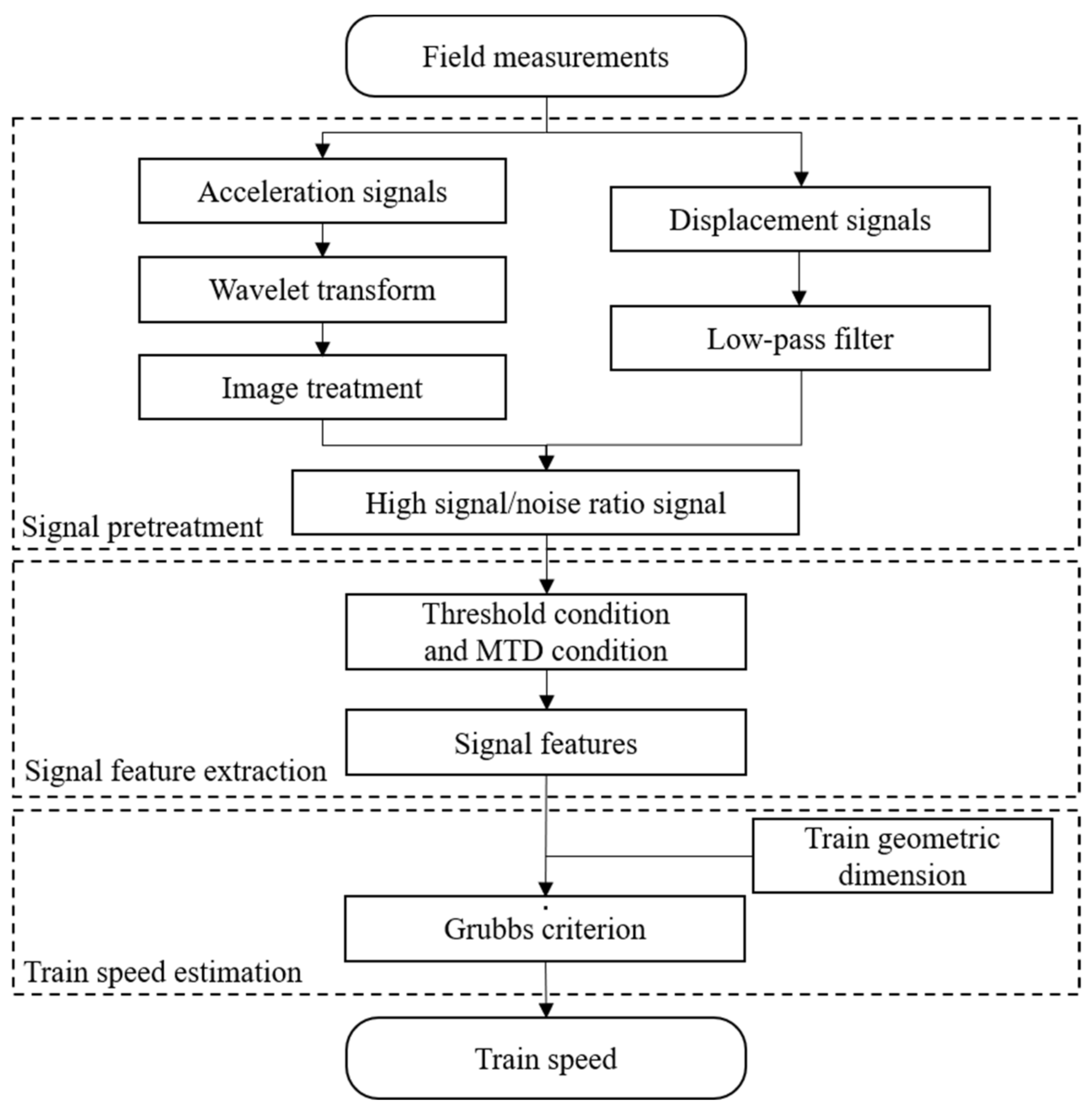
3. Procedures for Train Speed Estimation

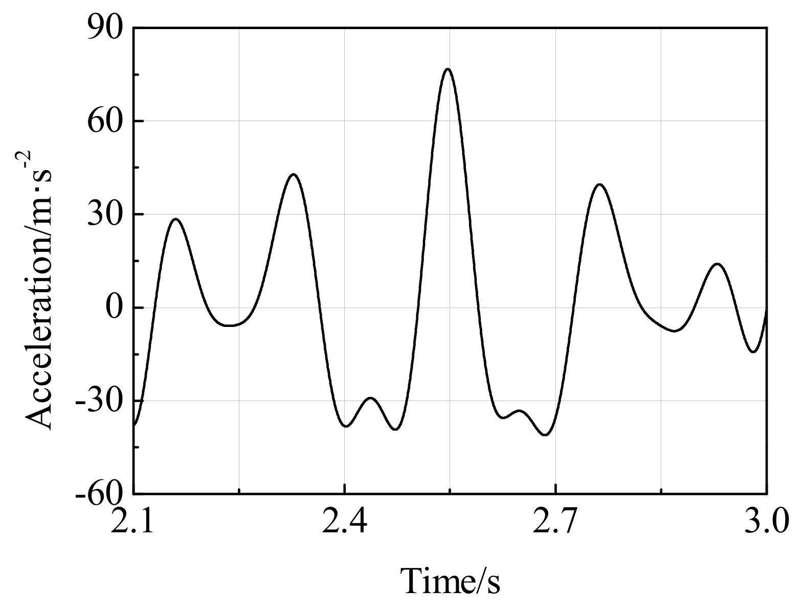
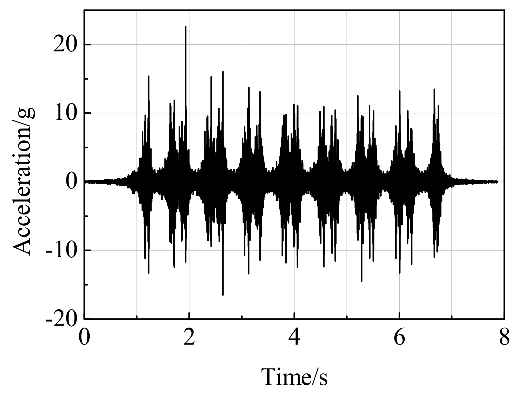
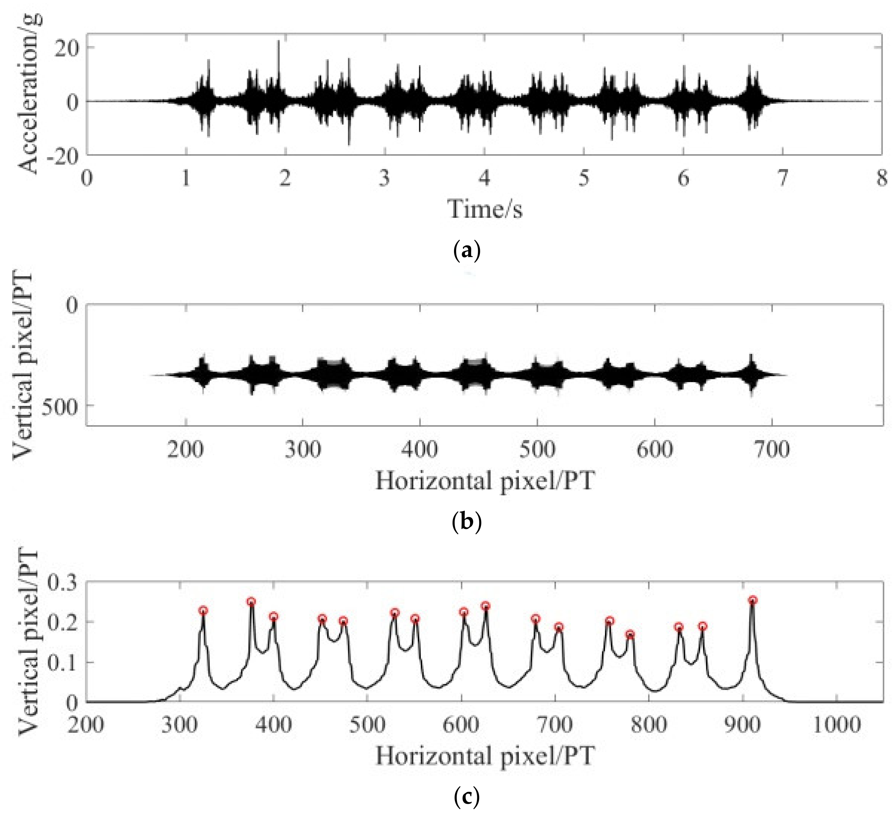
3.1. Train Speed Estimation from Acceleration Dynamic Response Signals

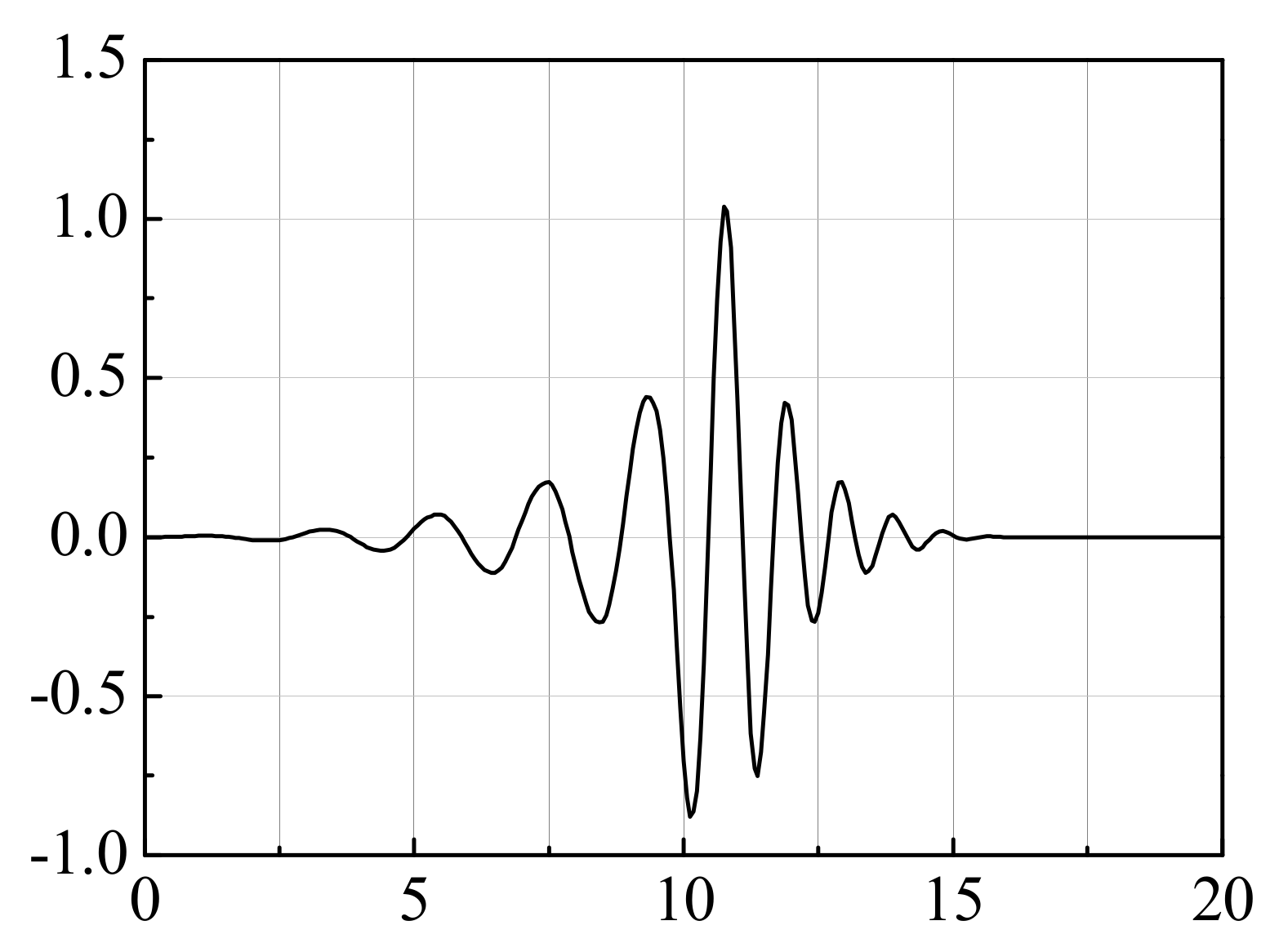
3.1.1. Signal Pretreatment

Figure 1a shows the typical time domain signals of vertical acceleration dynamic response of track structure. It can be seen from Figure 1 that the signal contains a lot of noise. Unfortunately, the true dynamic response signals and the disturbance signals are in the same frequency bands [18,19].
Wavelet transform, which inherits and develops the thought of localization of short-time Fourier transform, is a useful method of analyzing the non-stationary signals. It is the inner product of the wavelet basis function and the signals to be analyzed—that is, the signals are expressed as a linear combination of a series of wavelet functions with different scales and shifts. The coefficients of each term in the linear combination are called wavelet coefficients.
This paper selected the Mallat algorithm to calculate the discrete wavelet transform. The Mallat algorithm utilizes the multi-resolution characteristic of the wavelet to decompose the signal into two parts of the high-frequency D1 and the low-frequency A1. Then, the part of the low-frequency A1 is continually decomposed layer by layer to obtain the signal characteristics. The formula for the n-layer decomposition of the original signal S is as shown in Equation (2).
S = A n + D n + D n 1 + + D 1
The wavelet transform coefficients reflect the similarity between signal locality and the wavelet basis function. Accordingly, the shape of the selected wavelet basis function should be similar to that of the target signal. The vertical acceleration signal diagram with bogie information is as shown in Figure 3, which is obtained from the second derivative of the filtered vertical displacement signals. The Fejér–Korovkin wavelet with a length 22 filter (as shown in Figure 4) is selected as the base wavelet since the shapes and characteristics of the wavelet are similar to the vertical acceleration signals.
The original vertical acceleration signals are decomposed using the Fejér–Korovkin wavelet with a length 22 filter, and then the high-frequency signal D1 is recombined. As shown in Figure 5, the low-frequency interferences in the reconstructed signals are suppressed compared to the original signals in Figure 1a, but the high-frequency interferences still exist in the signal graph. Therefore, the signals need to be further processed to obtain signal features consistently.
After the wavelet transform, a mathematical morphological operation is performed on the binary image (Figure 5). The diamond structure element set S is selected, and the corrosion operation [20] is performed on the image. Then, the integrated grayscale vertical projection [21] is performed on the image after corrosion operation, and the grayscale change diagram is shown in Figure 6. Noteworthily, to ensure that the different signals can be transformed linearly after processing, all signals are intercepted with the same length.

3.1.2. Signal Feature Extraction

The track structure undergoes significant deformation when bogies pass through sensors, which produce obvious peaks in vertical acceleration waveform. In ideal status, each peak in the signals reflects one passing moment of one bogie. However, the filtered signals may still oscillate within a small range in field tests. To screen the effective peak points, the threshold condition and minimum time difference condition are proposed in this paper.
The threshold condition means that the amplitude of the possible effective peak needs to be greater than the critical value. It can effectively remove the peak points generating by the fluctuation while the amplitude of the signals is low. Assuming the maximum amplitude of the waveform is Amax, the amplitude of the possible effective peak needs to be greater than λAmax. It is noted that λ is defined as the threshold condition coefficient and its value range is [0, 1].
Based on the threshold condition, the minimum time difference condition is further presented to ensure that only one peak can be selected when one bogie passes through. Because the time difference of the adjacent bogies passing through the sensor is related to train length and speed, there is one minimum time difference between the adjacent effective peaks. When the maximum train speed at the test site is vmax, and the minimum bogie spacing is lmin, the minimum time difference parameter Δt should be meet the formula of Δt = lmin/vmax.
According to the above conditions, the peaks of the pretreated dynamic response waveforms are screened as shown in Figure 6c. According to the results shown in Figure 6c, it can be seen that the information of the bogie passing through is effectively conveyed by the waveforms, and then the passing time of bogies can be identified.

3.1.3. Train Speed Calculation

The train running speed can be calculated by combining the time of the bogie passing the sensor with the train dimension. The train dimension diagram is shown in Figure 7.
Applying the peak point screening method described above, the identified times of the train bogie passing through the sensor are t1, t2, …, tn. The time differences Δ T of adjacent bogies passing through are as shown in Equation (3):
Δ T = Δ t i = t i + 1 t i , i = 1 , 2 , , n 1
When the train speed v is constant, if la > lb, the time inferences can be divided into two categories, as shown in Equation (4):
Δ t a T a > Δ t ¯ > Δ t b T b
where Ta is the set of the time for the train to travel la (in Figure 7); Tb denotes the set of the time for the train to travel lb (in Figure 7); and Δ t ¯ is the sample average of Δ T . Then, the train speed is estimated in Equation (5):
V = l a T a l b T b
where V is the set of calculated train speeds. To avoid unpredictable situations in field tests, the Grubbs criterion is introduced to ensure the reliability of results. The Grubbs criterion is a method to distinguish abnormal values of samples obeying normal distribution when the total standard deviation σ(x) is unknown. It states that the data should be removed when the residual Vi corresponding to a measured value x satisfies Equation (6):
V i = x i x ¯ > g n , a × σ X
where x is the sample mean, g(n, a) is a coefficient depending on the number of measurements n, and the significance level a, σ(X) is the standard deviation of the sample. After judging by the Grubbs criterion, the average value of the remaining elements in set V is the final estimated train speed.

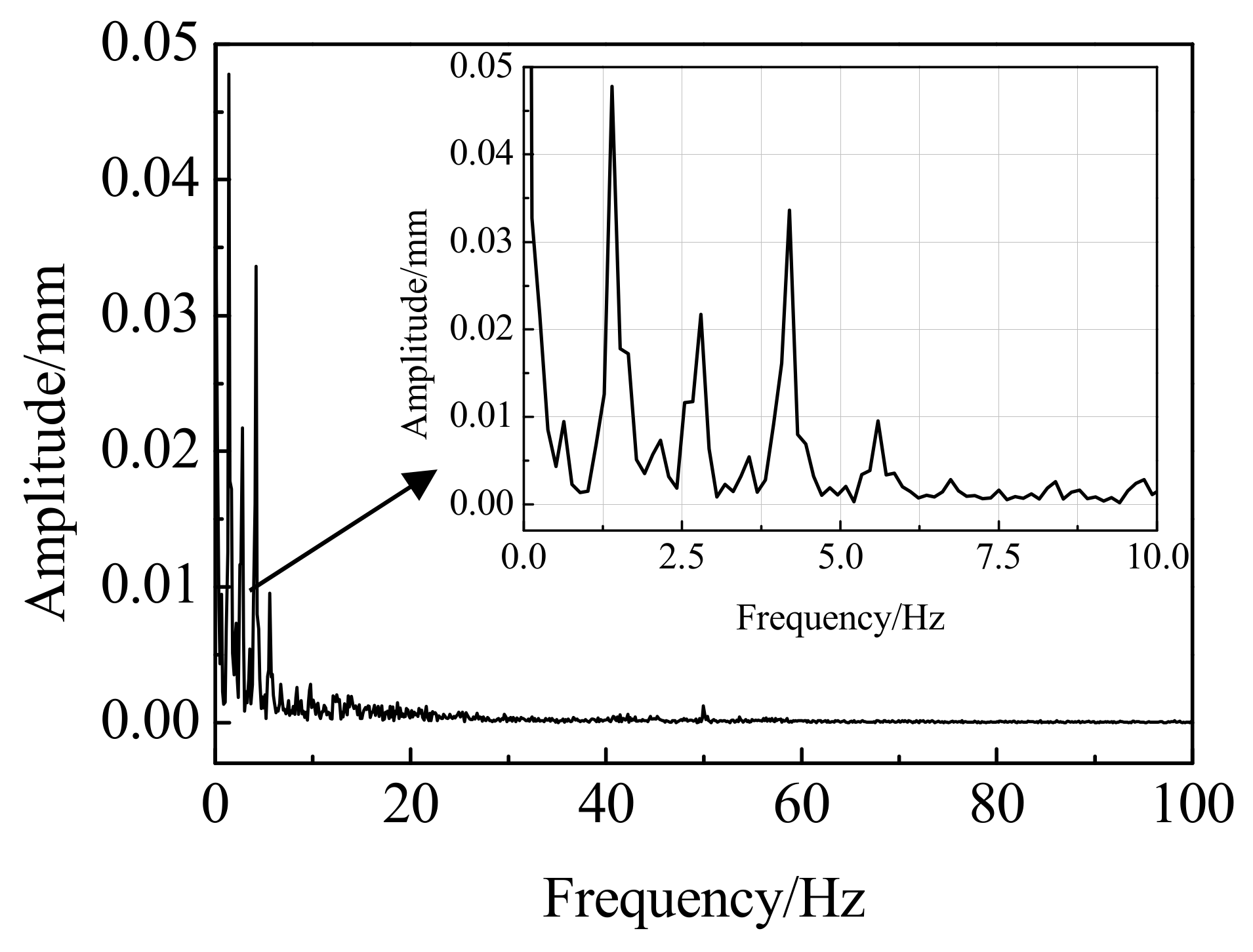
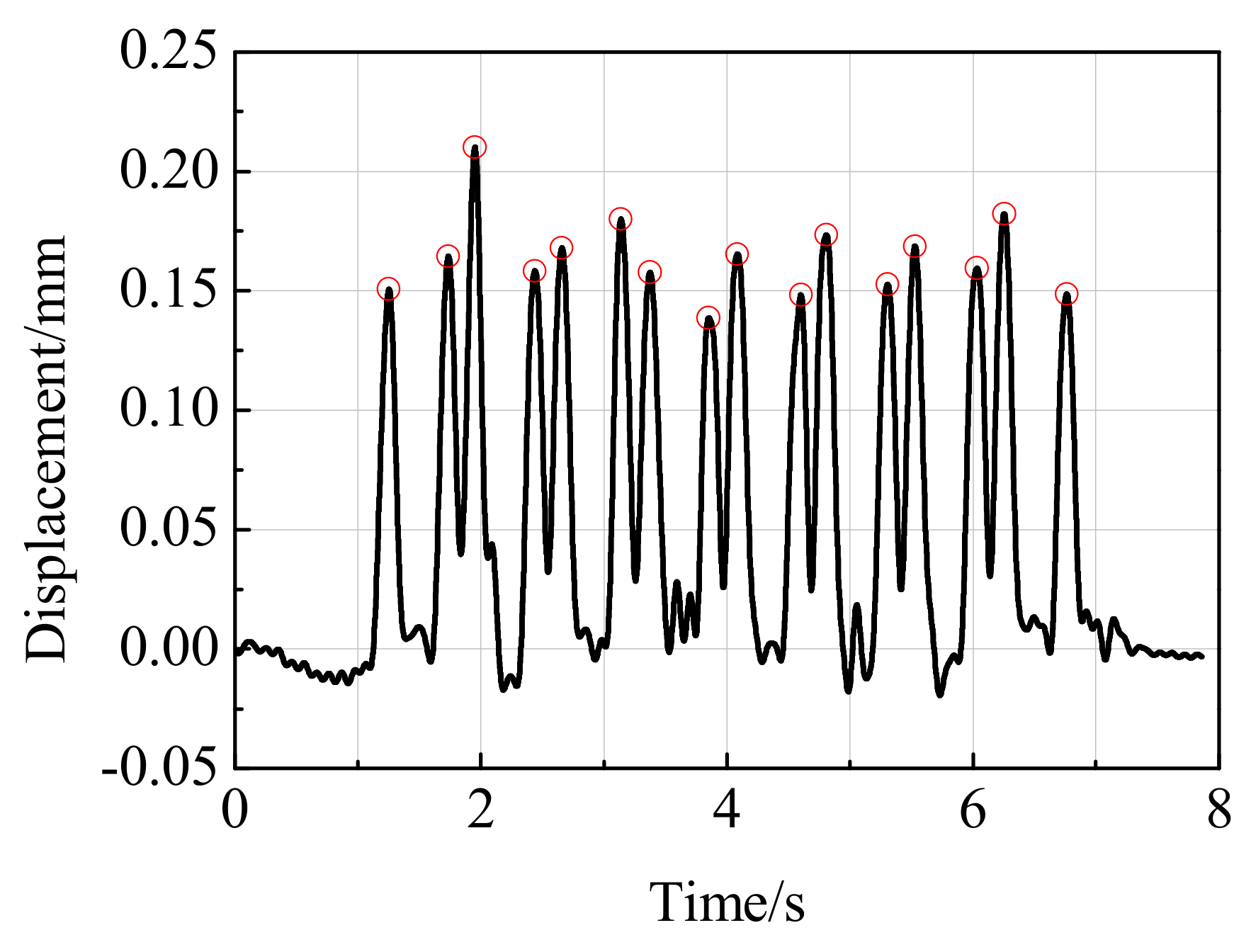
3.2. Train Speed Estimation from Displacement Dynamic Response Signals

Figure 1b and Figure 8 shows the typical time domain and frequency domain signals of vertical displacement dynamic response, respectively. It can be seen from Figure 8 that the signal contains a lot of noise. Furthermore, the true dynamic response signals and the disturbance signals are in different frequency bands.
Low-pass filtering (LPF) is thus chosen to suppress disturbance signals. To retain the characteristics of the signals, the cutoff frequency of the LPF should be greater than the frequency of the bogies passing through the sensors. Supposing that the train speed is v and the minimum spacing of adjacent bogies is lmin, the cutoff frequency fc should satisfy the condition of fcv/lmin. Figure 9 shows the low-pass filtered displacement signal. Compared to the original signal in Figure 1a, the noise and disturbance in vertical displacement–time waveform signals can be well suppressed, which meets the requirement of further signal feature extraction. The subsequent treatment is the same approach as that of the acceleration signals.

4. Verification of the Train Speed Estimation Method
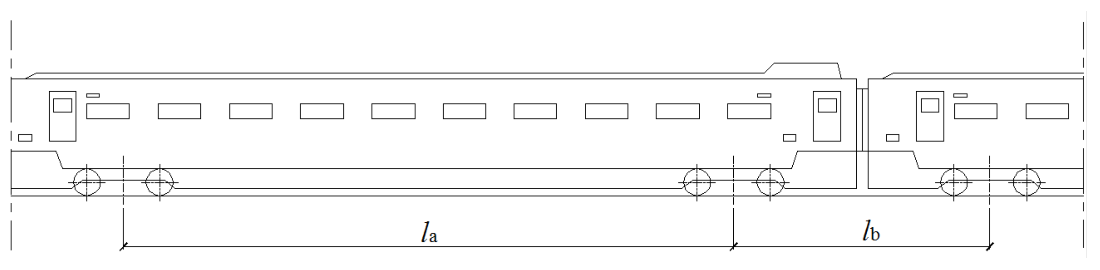
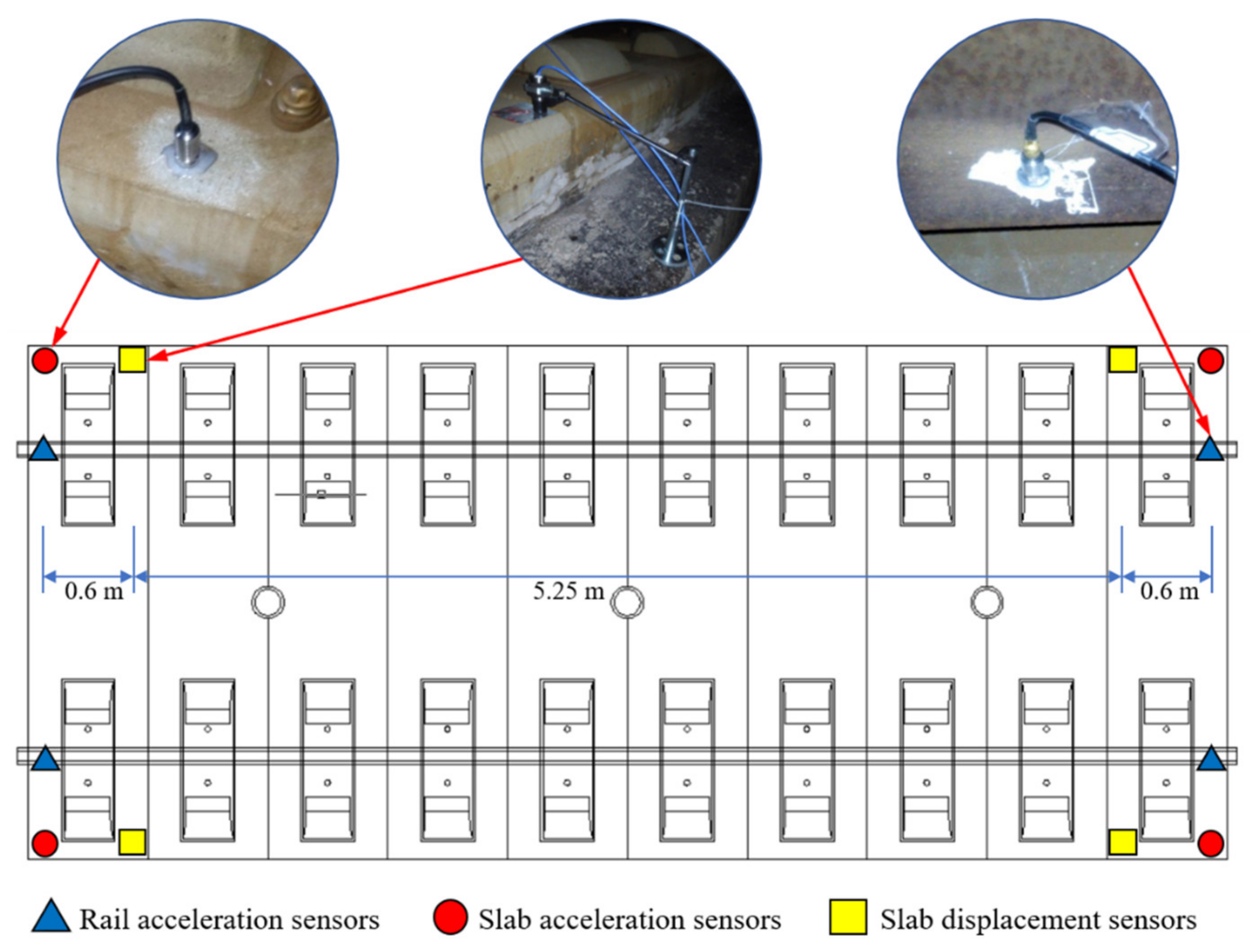
4.1. Test Overview

This paper uses the dynamic tests of China Railway High-speed (CRH) track as an example to verify the validity of the proposed train speed estimation algorithms. The dynamic test site was located on the bridge China Railway Track System II (CRTS II) slab ballastless track with a curve radius of 7000 m and an outer line height of 115 mm. The CRTS II slab ballastless track consists of rail with a grade of 60kg/m, elastic fastener, prefabricated track plate, mortar adjustment layer and supporting layer. The track slab is 2550 mm wide, 200 mm thick and 6450 mm long.
The rail acceleration was detected using a DH131E (with measuring range of 5000 m·s−2 and sensitivity of 1 mV·s−2) impedance converter accelerometer. The slab acceleration was detected using a DH187E (with measuring range of 1000 m·s−2 and sensitivity of 5 mV·s−2) impedance converter accelerometer. The vertical vibration of the slab displacement was detected using a DH821-10 (with measuring range of 10 mm and resolution of 0.005 mm) linear displacement sensor. The slab acceleration was detected using a DH187E impedance converter accelerometer. The sensors were pasted on the cleaned rail and track slab, as shown in Figure 10. All the test signals were collected using a DH5902 dynamic data acquisition device at a sampling frequency of 10k Hz. The sensors and the device were produced by Donghua Testing Technology Co., Ltd., Taizhou, Jiangsu, China. The sensor arrangement is shown in Figure 10 and Table 2, respectively. There is a gap between the slab and the support layer at one wide and narrow joint while the other side is healthy.
The trains in the test are all CRH series high-speed trains. As shown in Figure 7, the center distance of the bogies in the same carriages la is 17.5 m and the center distance of the bogies in adjacent carriages lb is 7.5 m. The threshold condition coefficient λ of slab displacement, slab acceleration, and rail acceleration is taken as 0.6, 0.4, and 0.3, respectively. The significance level of the Grubbs criterion is equal to 0.05.

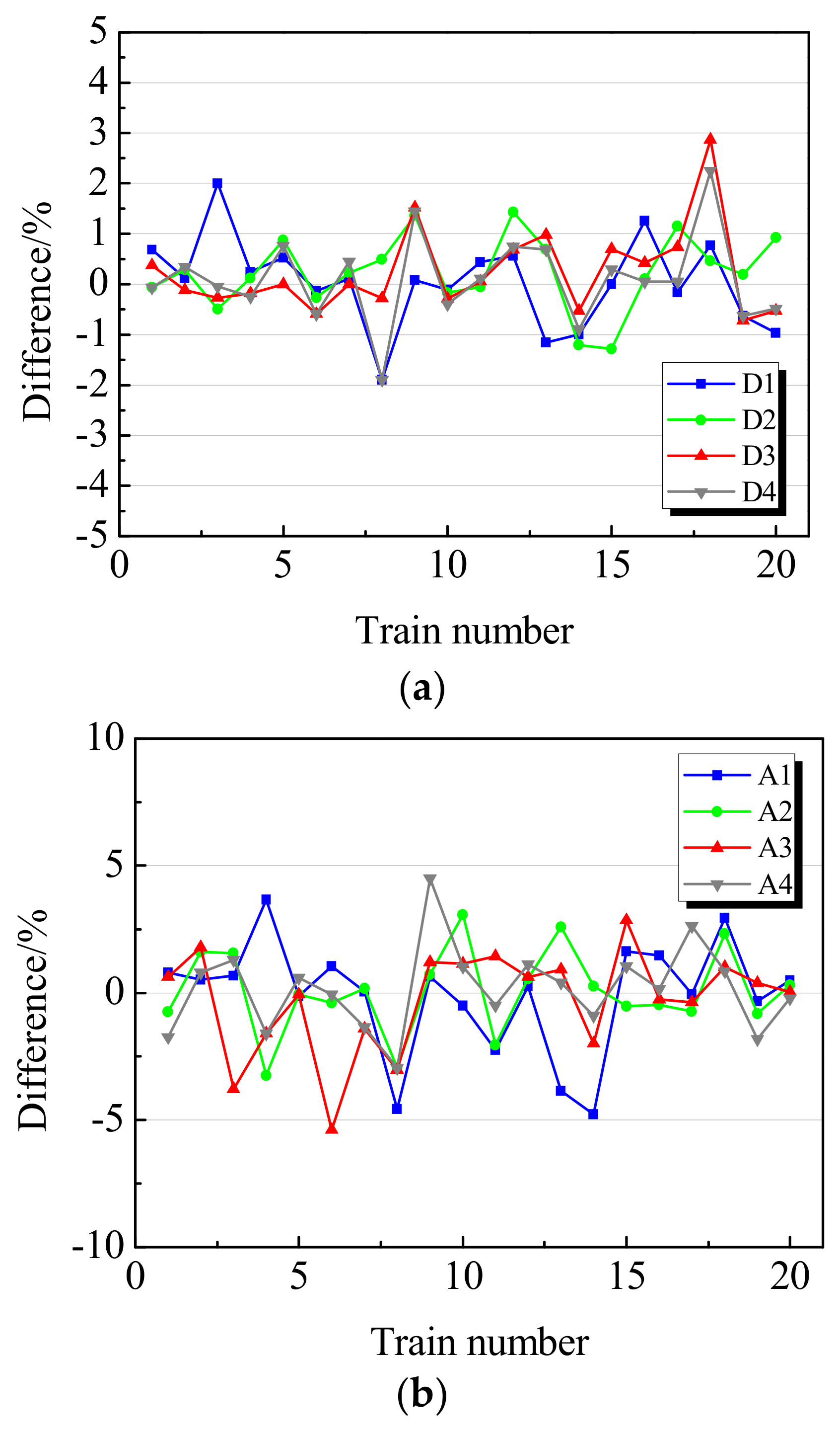
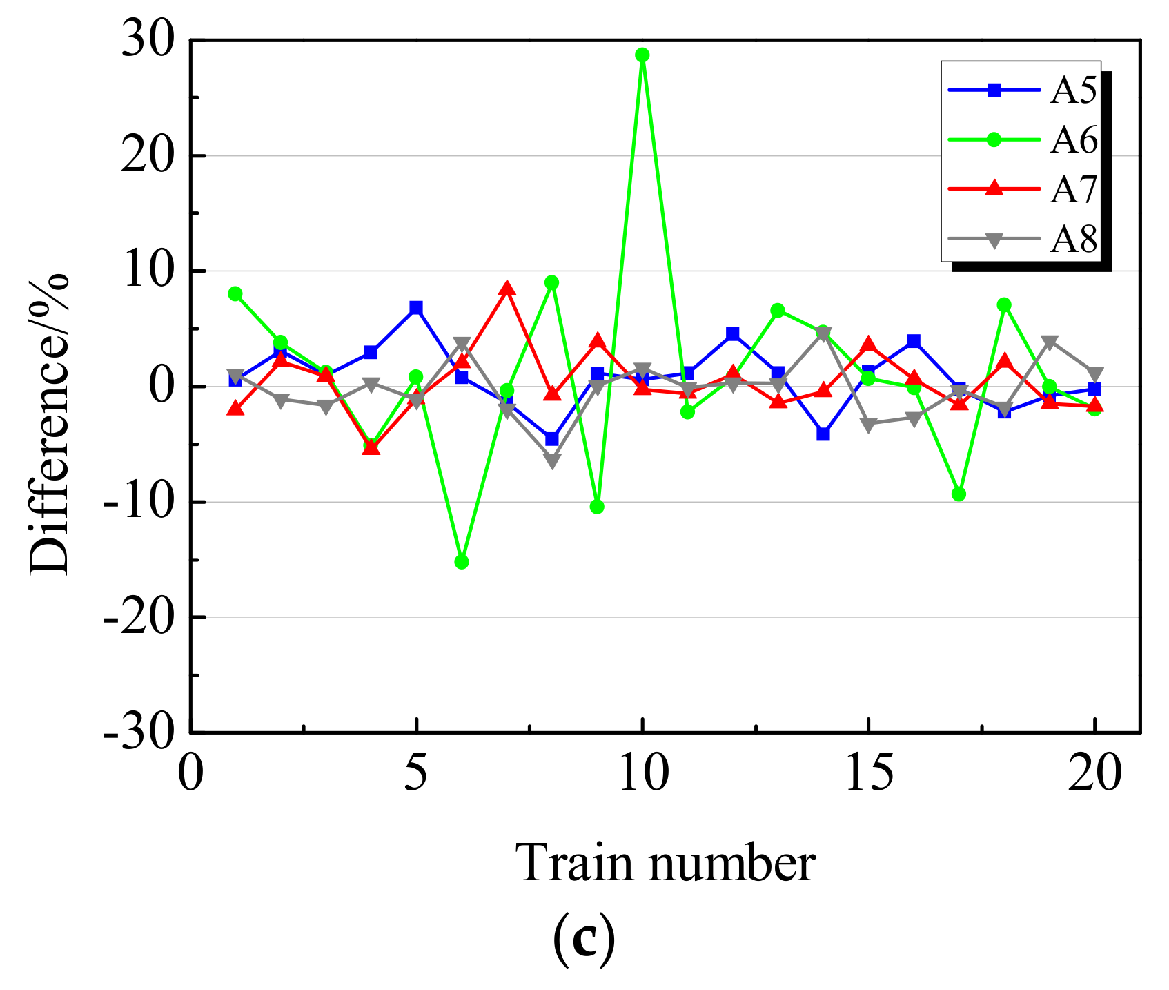
4.2. Train Speed Estimation Results
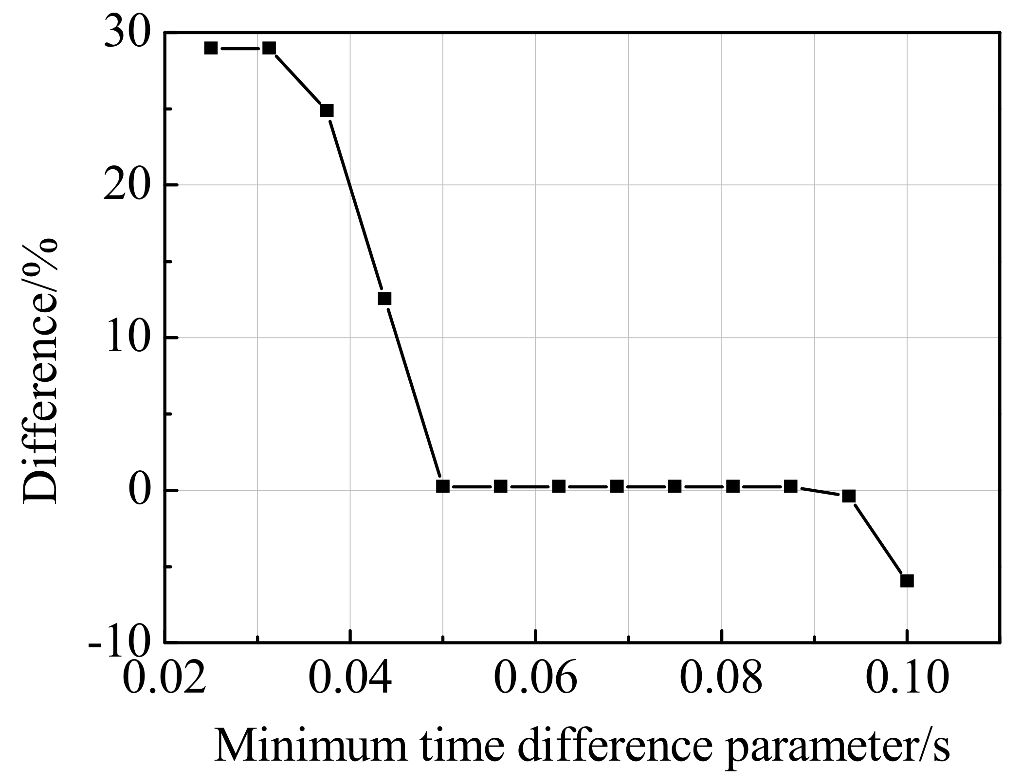
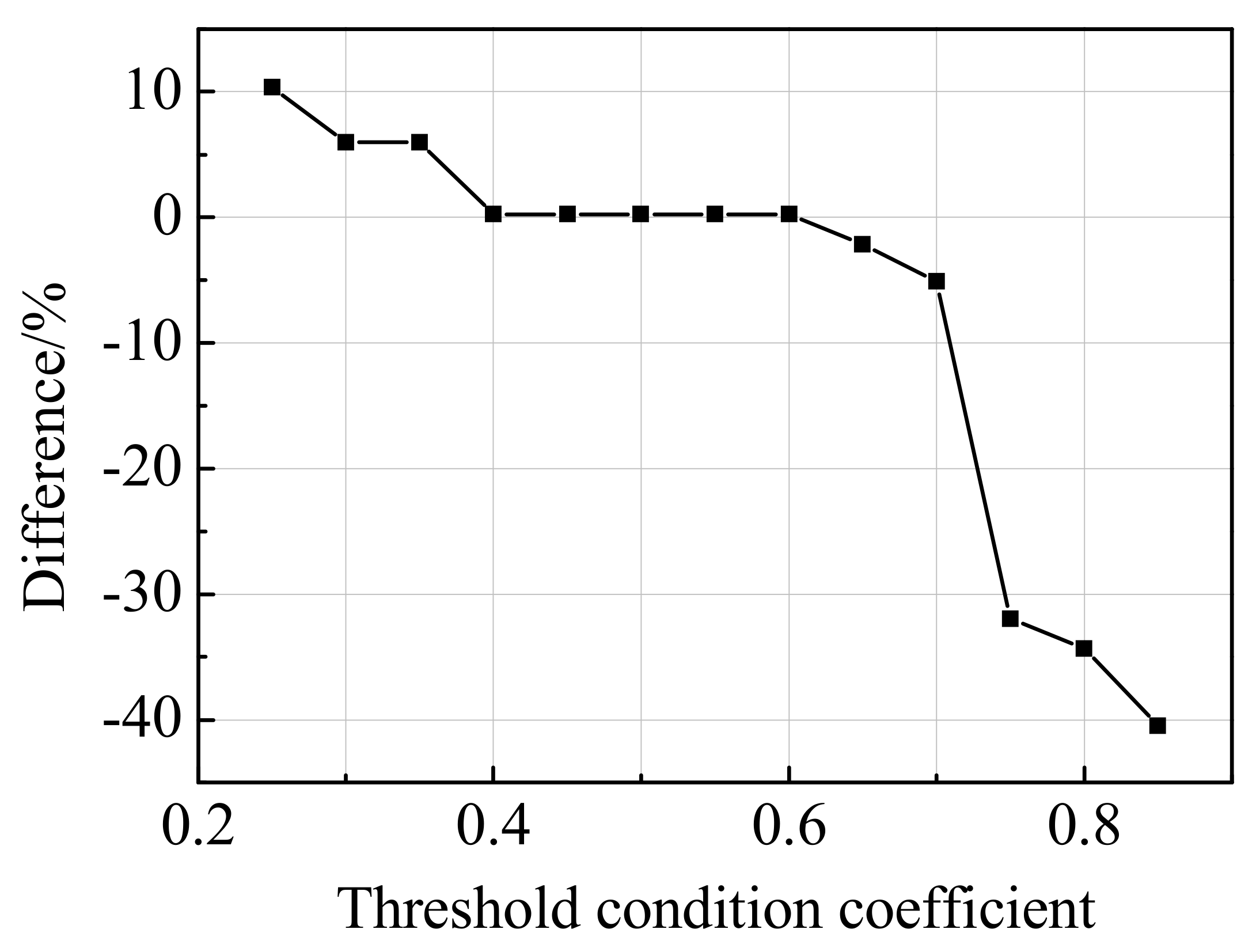
In this paper, twenty passing trains are used to identify the reliability of the method by using the displacement of the track slab, the acceleration of the track slab, and the acceleration of the rail. The relative difference δ of the proposed method can be calculated by Equation (7):
δ = V v V T V T × 100 %
where Vg is the train speed estimated from track structure vibration measurements and VT is the true train speed. The train speeds ranged from 124.6 km/h to 227.2 km/h, which were estimated using the proposed method and wheel counter. The train speed estimated using the wheel counter is assumed as the true value because the wheel counter is very accurate [16,22].
As shown in Figure 11, the relative differences of the proposed method are mostly less than 2% based on slab displacement, 5% based on rail acceleration, and 10% based on slab acceleration, respectively. The absolute average differences are listed in Table 3. It is apparent from the table that the slab displacement signals are very stable regardless of the sensor position and the track structure situation. The results of the rail acceleration can be affected by the track structure situation. The accuracy of estimation results is improved lightly when a gap between the slab and the support layer exists. In contrast, the existing gap seems to amplify the differences in the slab acceleration estimation results. Furthermore, the estimation results may be not influenced by the track curve. In summary, the validation results show that this proposed method can effectively estimate the train speed.

4.3. Discussions

Although it is proved that the speeds of all trains can be accurately estimated with unchanged parameters, different threshold condition coefficients and the minimum time difference parameters are also discussed in Table 4 for improving the applicability of the method. It can be seen from the data in Table 4 that the accuracy of train speed estimation is influenced by the threshold condition coefficient and the minimum time difference parameter. Therefore, the results of train speed automatic estimation will be significantly improved if the parameter is selected dynamically and accurately. As the appropriate parameters are related to the train speed, it is necessary to roughly estimate the train speed first to determine the appropriate parameters.
Figure 12 shows the minimum time difference parameter on the results of train speed estimation. It can be concluded that the difference decreases notably when the minimum time difference parameter is higher than the time difference of adjacent bogies passing through the measuring site. Therefore, it is necessary to ensure that the minimum time difference parameter is greater than the time difference of adjacent bogies passing through the measuring points. In this paper, there are two types of trains: some of them with eight carriages trains and others with sixteen carriages. The train speed can be roughly estimated by the combination of the total length of the train and the total time of signals. Computer vision will still be a useful application for the problem. The acceleration signal image gives the number of train carriages by the number of closed regions. This method was used in the fields of fish fry counting [23], pest counting [24], cell counting [25], and distinguishing parking spaces [26], and it has achieved good results. Furthermore, displacement signals can be used to estimate train speed as long as a histogram is used instead of a line graph. After rough estimation of train speed, the minimum time difference parameter can be determined as detailed in Section 3.1.2.
As shown in Figure 13, the difference is quite small, as the threshold condition coefficient is equal to 0.4–0.6. When the parameters are higher than 0.6, the number of identified peaks will be significantly reduced. Using this feature, the threshold condition coefficient can be designed to be self-adjusted dynamically. When the threshold condition coefficient is 1, only one peak point can be selected at this time, and more peak points can be selected with decreasing the coefficient. After the train carriage information is obtained, the number N of train bogies is determined, so the coefficients can be dynamically valued from large to small until N peak points are selected. Therefore, the coefficients of the method can be easily calibrated based on the numbers of identified bogies and the relationship between minimum time difference parameter and estimated train speed. In addition, after all peak points have been selected, the critical value of the Grubbs criterion can be appropriately tightened to improve the accuracy of recognition.
The proposed method can be applied extensively under two conditions. First, the signal waveform of vertical acceleration and displacement produce pronounced peaks when the rail wheels pass through the test site. According to previous studies [27,28,29,30,31], it can be deduced that it is quite possible to estimate train speed from the vibration measurements of both ballastless track and ballast track with this method. Second, the proposed method needs all the passing trains to have the same geometric dimensions.

5. Conclusions

This paper proposed a train speed estimation method by extracting the characteristics of the vibration measurements of rail acceleration, slab acceleration, and slab displacement. The train speed can be automatically and reliably calculated by the combination of the extracted characteristics and the geometric dimension of the train. The results showed that the average differences of the train speed calculated by phase differences and the proposed method were 0.61% for slab displacement measurements, 1.39% for rail acceleration measurements, and 2.97% for slab acceleration measurements. In addition, the method is stable regardless of the sensor position and the track structure situation.
The proposed method can be applied extensively under two conditions: the signal waveform of vertical acceleration and displacement produce pronounced peaks when the rail wheels pass through the test site, and all the passing trains have the same geometric dimensions. Therefore, this method offers an efficient way for track structural health monitoring to obtain the train speed from track structure vibration measurements without additional speed measurement module. The method meets the requirement of speed estimation in the short-term, multi-location, and tough environment of structural health monitoring. Noteworthily, it is also a successful attempt to introduce image processing technology into high speed rail. This idea can be further applied to railway analysis to make up the insufficiency of tradition signal processing methods.

Author Contributions

Conceptualization, X.W. and X.S.; Methodology, X.W. and J.W.; Validation, X.W.; Funding acquisition, X.S. and B.H.; Investigation, X.W., J.W., and X.Y.; Project administration, X.S. and B.H.; Supervision, X.S., X.Y., and B.H.; Writing—original draft, X.W. and J.W.; Writing—review & editing, X.S., X.Y. and B.H. All authors have read and agreed to the published version of the manuscript.

Funding

This research was funded by the Natural Science Foundation of Hebei province (E2019210264) and the Fundamental Research Funds for the Central Universities in China (DUT18GJ203). And the APC was funded by the Natural Science Foundation of Hebei province (E2019210264).

Acknowledgments

The authors thank the funding supported from the Natural Science Foundation of Hebei province (E2019210264) and the Fundamental Research Funds for the Central Universities in China (DUT18GJ203).

Conflicts of Interest

The authors declare no conflict of interest.

References

  1. Zhou, L.; Wei, T.; Zhang, G.; Zhang, Y.; Gildas, M.A.; Zhao, L.; Guo, W. Experimental Study of the Influence of Extremely Repeated Thermal Loading on a Ballastless Slab Track-Bridge Structure. Appl. Sci. 2020, 10, 461. [Google Scholar] [CrossRef] [Green Version]
  2. Mosleh, A.; Costa, P.A.; Calcada, R. A new strategy to estimate static loads for the dynamic weighing in motion of railway vehicles. Proc. Inst. Mech. Eng. Part F J. Rail Rapid Transit 2019, 234, 183–200. [Google Scholar] [CrossRef]
  3. Poisson, F.; Gautier, P.E.; Letourneaux, F. Noise sources for high speed trains: A review of results in the TGV case. In Noise and Vibration Mitigation for Rail Transportation Systems; Springer: Berlin/Heidelberg, Germany, 2008; pp. 71–77. [Google Scholar]
  4. Kouroussis, G.; Connolly, D.; Verlinden, O. Railway-induced ground vibrations—A review of vehicle effects. Int. J. Rail Transp. 2014, 2, 69–110. [Google Scholar] [CrossRef] [Green Version]
  5. Auersch, L. Theoretical and Experimental Excitation Force Spectra for Railway-Induced Ground Vibration: Vehicle-Track-Soil Interaction, Irregularities and Soil Measurements. Veh. Syst. Dyn. 2010, 48, 235–261. [Google Scholar] [CrossRef]
  6. Li, H.; Wu, G. Fatigue evaluation of steel bridge details integrating multi-scale dynamic analysis of coupled 0train-track-bridge system and fracture mechanics. Appl. Sci. 2020, 10, 3261. [Google Scholar] [CrossRef]
  7. Galvan, E.; Torralba, A.; Franquelo, L.G. ASIC implementation of a digital tachometer with high precision in a wide speed range. IEEE Trans. Ind. Electron. 1996, 43, 655–660. [Google Scholar] [CrossRef]
  8. Chandrasekaran, G.; Vu, T.; Varshavsky, A.; Gruteser, M.; Martin, R.P.; Yang, J.; Chen, Y. Vehicular speed estimation using received signal strength from mobile phones. In Proceedings of the ACM International Conference on Ubiquitous Computing, Copenhagen, Denmark, 26–29 September 2010. [Google Scholar]
  9. Connolly, D.; Kouroussis, G.; Woodward, P.K.; Costa, P.A.; Verlinden, O.; Forde, M.C. Field testing and analysis of high speed rail vibrations. Soil Dyn. Earthq. Eng. 2014, 67, 102–118. [Google Scholar] [CrossRef] [Green Version]
  10. Marinov, M.; Hensel, S.; Strau, T. Eddy current sensor based velocity and distance estimation in rail vehicles. IET Sci. Meas. Technol. 2015, 9, 875–881. [Google Scholar] [CrossRef]
  11. Liu, C.; Liu, H.; Guo, Y.; Liu, M.; Zhang, B.; Ye, S. Train speed measurement system based on the scanning laser radar. China Railw. Sci. 2009, 30, 7–13. [Google Scholar]
  12. Auersch, L. Ground vibration due to railway traffic-the calculation of the effects of moving static loads and their experimental verification. J. Sound Vib. 2006, 293, 599–610. [Google Scholar] [CrossRef]
  13. Lombaert, G.; Degrande, G. Ground-borne vibration due to static and dynamic axle loads of InterCity and high-speed trains. J. Sound Vib. 2009, 319, 1036–1066. [Google Scholar] [CrossRef]
  14. Ni, S.H.; Huang, Y.H.; Lo, K.F. An automatic procedure for train speed evaluation by the dominant frequency method. Comput. Geotech. 2011, 38, 416–422. [Google Scholar] [CrossRef]
  15. Kouroussis, G.; Connolly, D.P.; Laghrouche, O.; Forde, M.C.; Woodward, P.K.; Verlinden, O. Robustness of railway rolling stock speed calculation using ground vibration measurements. In MATEC Web of Conferences; paper no. 20: 07002; EDP Sciences: Amsterdam, The Netherlands, 2015. [Google Scholar]
  16. Kouroussis, G.; Connolly, D.P.; Forde, M.C.; Verlinden, O. Train speed calculation using ground vibrations. Proc. Inst. Mech. Eng. Part F J. Rail Rapid Transit 2015, 229, 466–483. [Google Scholar] [CrossRef] [Green Version]
  17. Murthy, C.B.; Hashmi, M.F.; Bokde, N.D.; Geem, Z.W. Investigations of object detection in images/videos using various deep learning techniques and embedded platforms—A comprehensive review. Appl. Sci. 2020, 10, 3280. [Google Scholar] [CrossRef]
  18. Ju, S.H.; Lin, H.T.; Huang, J.Y. Dominant frequencies of train-induced vibrations. J. Sound Vib. 2009, 319, 247–259. [Google Scholar] [CrossRef]
  19. Wang, Z.; Ling, X.; Zhu, Z.; Zhang, F. Dominant frequencies of train-induced vibrations in a seasonally frozen region. Cold Regions Sci. Technol. 2015, 116, 32–39. [Google Scholar] [CrossRef]
  20. Forsyth, D.A.; Ponce, J. Computer Vision A Modern Approach, 2nd ed.; Pearson: New York, NY, USA, 2012. [Google Scholar]
  21. Huang, Z.; Wang, R.; Shan, S.; Chen, X. Projection Metric Learning on Grassmann Manifold with Application to Video based Face Recognition. In Proceedings of the Computer Vision & Pattern Recognition, Boston, MA, USA, 7–12 June 2015. [Google Scholar]
  22. Vega, J.; Fraile, A.; Alarcon, E.; Hermanns, L. Dynamic response of underpasses for high-speed train lines. J. Sound Vib. 2012, 331, 5125–5140. [Google Scholar] [CrossRef] [Green Version]
  23. Labuguen, R.T.; Volante, E.J.P.; Causo, A.; Bayot, R.; Peren, G.; Macaraig, R.M.; Libatique, N.J.C.; Tangonan, G.L. Automated fish fry counting and schooling behavior analysis using computer vision. In Proceedings of the IEEE International Colloquium on Signal Processing & Its Applications, Malacca, Malaysia, 23–25 March 2012. [Google Scholar]
  24. Li, W.; Li, M.; Chen, M.; Quian, J.; Sun, C.; Du, S. Feature extraction and classification method of multi-pose pests using machine vision. Trans. Chin. Soc. Agric. Eng. 2014, 30, 154–162. [Google Scholar]
  25. Yuan, W.; Zhang, T. A counter method for the image of blood cell. Comput. Appl. Softw. 2000, 17, 61–64. [Google Scholar]
  26. Ma, S.; Jiang, Z.; Jiang, H.; Han, M.; Li, C. Parking space and obstacle detection based on a vision sensor and checkerboard grid laser. Appl. Sci. 2020, 10, 2582. [Google Scholar] [CrossRef] [Green Version]
  27. Liu, L.; Song, R.; Zhou, Y.; Qin, J. Noise and vibration mitigation performance of damping pad under CRTS-III ballastless track in high speed rail viaduct. KSCE J. Civ. Eng. 2019, 23, 3525–3534. [Google Scholar] [CrossRef]
  28. Galvin, P.; Romero, A.; Dominguez, J. Vibrations induced by HST passage on ballast and non-ballast tracks. Soil Dyn. Earthq. Eng. 2010, 30, 862–873. [Google Scholar] [CrossRef] [Green Version]
  29. Gupta, S.; Liu, W.; Degrande, G.; Lombaert, G.; Liu, W. Prediction of vibrations induced by underground railway traffic in Beijing. J. Sound Vib. 2008, 310, 608–630. [Google Scholar] [CrossRef]
  30. Nishiura, D.; Sakai, H.; Aikawa, A.; Tsuzuki, S.; Sakaguchi, H. Novel discrete element modeling coupled with finite element method for investigating ballasted railway track dynamics. Comput. Geotech. 2017, 40–54. [Google Scholar] [CrossRef]
  31. Mishra, D.; Qian, Y.; Huang, H.; Tutumluer, E. An integrated approach to dynamic analysis of railroad track transitions behavior. Transp. Geotech. 2014, 1, 188–200. [Google Scholar] [CrossRef]
Figure 1. The typical dynamic response waveform: (a) displacement; (b) acceleration.
Applsci 10 04742 g001
Figure 2. The framework of the proposed train speed estimation algorithm.
Applsci 10 04742 g002
Figure 3. Acceleration waveform diagram containing bogie information.
Applsci 10 04742 g003
Figure 4. Fejér–Korovkin wavelet with a length 22 filter.
Applsci 10 04742 g004
Figure 5. High-frequency D1 signal recombination waveform.
Applsci 10 04742 g005
Figure 6. Diagrams of image treatment process: (a) the high-frequency D1 signal recombination waveform diagram; (b) the corrosive operated waveform diagram; (c) the gray vertical projection and the signal feature extraction results.
Applsci 10 04742 g006
Figure 7. The geometric dimension of the train.
Applsci 10 04742 g007
Figure 8. Frequency domain diagram of vertical displacement dynamic response signals.
Applsci 10 04742 g008
Figure 9. Low-pass filtered displacement signals (the red circle indicates the passing moments of the train bogies).
Applsci 10 04742 g009
Figure 10. Sensor location diagram.
Applsci 10 04742 g010
Figure 11. The automatic train speed estimation results of (a) the slab displacement, (b) the rail acceleration, and (c) the slab acceleration, respectively.
Applsci 10 04742 g011aApplsci 10 04742 g011b
Figure 12. The difference of results of train speed estimation with different minimum time difference parameters.
Applsci 10 04742 g012
Figure 13. The difference of results of train speed estimation with different threshold condition coefficients.
Applsci 10 04742 g013
Table 1. Existing methods for train speed estimation.
MethodTest LocationAdvantageShortcomingError
TachometersOn-boardNo additional measurementUsing inside the train~5%
GPSOn-boardCheapUsing inside the train5–10%
Optical sensorsGroundVery accurateAffected by weather especially rain and snow<1%
Wheel countersGroundVery accurateStationary application<1%
Eddy current sensorsGroundAccurateAffecting by rail structure state~1%
Laser radar systemGroundEasy to useAccuracy dependingon the position1–5%
Table 2. The sensor arrangement.
SensorLocationContentThe Track CurveStructure State
D1SlabDisplacementInsideHealthy
D2SlabDisplacementInsideLayer gap
D3SlabDisplacementOutsideHealthy
D4SlabDisplacementOutsideLayer gap
A1RailAccelerationInsideHealthy
A2RailAccelerationInsideLayer gap
A3RailAccelerationOutsideHealthy
A4RailAccelerationOutsideLayer gap
A5SlabAccelerationInsideHealthy
A6SlabAccelerationInsideLayer gap
A7SlabAccelerationOutsideHealthy
A8SlabAccelerationOutsideLayer gap
Table 3. Absolute average differences of different sensors.
SensorAbsolute Average Differences/%SensorAbsolute Average Differences/%
D10.64A31.49
D20.59A41.28
D30.59A52.12
D40.62A65.81
A11.53A72.08
A21.26A81.87
Table 4. The results of automatic train speed estimation with different parameters.
Train NumberSensorThreshold Condition CoefficientMinimum Time Difference Parameter/sEstimated Train Speed/km·h−1Difference/%
9A10.30.1124.70.1
9A10.10.1255.4105.0
9A10.50.1125.40.6
9A10.30.05149.019.6
9A10.30.2125.40.6
20A10.30.1228.80.7
20A10.10.1235.03.4
20A10.50.1228.80.7
20A10.30.05228.30.5
20A10.30.2111.7−50.8

