Article

Tolerance Design and Robust Study for The Joint Clearances of Landing Gear Retraction Mechanisms

1
Key Laboratory of Fundamental Science for National Defense-Advanced Design Technology of Flight Vehicle, Nanjing University of Aeronautics and Astronautics, Nanjing 210001, China
2
State Key Laboratory of Mechanics and Control of Mechanical Structures, Nanjing University of Aeronautics and Astronautics, Nanjing 210001, China
*
Author to whom correspondence should be addressed.
These authors contributed equally to this work.
Appl. Sci. 2020, 10(14), 4856; https://doi.org/10.3390/app10144856
Submission received: 8 June 2020 / Revised: 10 July 2020 / Accepted: 11 July 2020 / Published: 15 July 2020
(This article belongs to the Section Mechanical Engineering)

Abstract

:

Featured Application

Tolerance design is an essential process for a landing gear retraction mechanism. The results of the tolerance design would affect joint clearances, as well as the kinematic accuracy and robustness of the mechanism. The work presented here can be applied in the tolerance design of landing gear retraction mechanisms. It can also be used to analyze the kinematic accuracy and robustness of complicated mechanisms.

Abstract

Joint clearances inevitably affect the kinematic accuracy and robustness of landing gear retraction mechanisms. However, the complexity and uncertainty of the clearances lead to difficulty in establishing mathematic models and analyzing effects. In the interest of assessing the clearance effects on the kinematic accuracy of landing gears, an integrated tolerance theory is proposed in this paper. In the theory proposed, Jacobian–Torsor model is combined with robust analysis to establish the kinematic accuracy model and predict the influences of clearances. The overall steps to apply the theory presented in practice are given. A typical landing gear retraction mechanism is chosen for the case study and the results show that the tendencies of clearances can be observed. Through the process of tolerance design, robust study, and tolerance redesign, the kinematic accuracy is significantly improved. The integrated tolerance theory proposed and the study conducted will provide designers new insights for the clearance analysis of landing gear mechanisms.

1. Introduction

During the phases of take-off and landing of the flight, the main task of a landing gear retraction mechanism is to extend the structure stably and precisely to the designated position [1,2]. The stability and precision of a landing gear mechanism are strongly concerned with its robustness. Joint clearances are universal for landing gears, and they inevitably affect the kinematic accuracy and robustness of mechanisms. Due to the uncertainty and complexity of clearances, it is often challenging to model them in the kinematic analysis. And what is more, this situation results in the difficulty to estimate the joint clearance effects on the kinematic accuracy and robustness.
Traditionally, the kinematic accuracy model is deduced from the kinematic equations, however, joint clearances are often omitted. There is a relative paucity of studies focusing specifically on the relations between clearance effects and kinematic accuracy. Meanwhile, no previous study has covered the robustness of a mechanism through the way of kinematic accuracy analysis. An intriguing question is raised, that is, how to establish the link among joint clearances, kinematic accuracy, and robustness. The answer in this paper is tolerance analysis.
Regarding aircraft assemblies, dimensional chains are widely used in tolerance analysis. Basic theories are described in the literature written by B.Q. Cheng [3]. Jacobian model is a novel method in tolerance theory, which was proposed by Luc Laperriere and Philippe Lafond [4,5,6]. In this model, Functional element (FE) pairs and functional requirement (FR) are used to represent the relationship between parts. Tolerance propagation functions are obtained by transform matrix of variations. The utilization of this model has been expanded in the past twenty years. A. Desorchers, A. Riviere, and W. Ghie [7,8,9,10,11] modified the original Jacobian model and established Jacobian–Torsor model. Different joint types are represented by the displacement matrix in the model. Meanwhile, tolerance zones and propagation functions can be established by this model. Many studies [12,13,14,15,16,17,18,19] have involved the application of these two jacobian models. In the manufacturing process, the study of X.Y.Zou [20] treated workpieces, fixtures, and machine tools as an assembly, and formulated the corresponding error propagation model using the Jacobian–Torsor theories. A group of constraints to variations were added to the Jacobian–Torsor model by H. Chen [21,22,23]. The analysis of engine assemblies was performed by this modified model in his study. Concerning kinematic accuracy analysis, the small-displacement torsor model was used in the study conducted by X. Zhou [24]. However, the application was still bound up with the static assembly processing, which limits the use of tolerance theory. The Jacobian model is the ideal method to establish a kinematic accuracy model for mechanisms, however, efforts are lacking thus far.
Robustness is the idea first proposed in the area of product quality and widely adopted in various industrial fields [25]. On the subject of mechanism design, several studies have tried to introduce robust theories into parameter analysis [26,27,28,29,30,31,32]. The target of robust analysis is to get high-quality design insensitive to unexpected errors and deviations. Caro Stephane et al [33] proposed to adopt robust theories to find an appropriate robustness index, and then robust dimensions can be obtained. The Taguchi method in robust theory was utilized to obtain a set of robot parameters and to reduce performance variations by Rout and Mittal [34]. In the study by Dua et al [35], random and interval variables were considered and then performance deviations were minimized through the robust mechanism synthesis. Similarly, the study by Luo et al [36] proposed to accommodate truncated random variables and clearance variables during robust design. The Taguchi method was improved especially for mechanisms by Huang and Zhang [37,38]. In their study, the method was used to determine the optimal tolerances for individual components of mechanisms. To date, robust theories have not been utilized in the tolerance and clearance analysis for landing gears.
The primary aim of this paper is to propose an integrated theory to analyze the clearance effects on the kinematic accuracy of landing gear mechanisms and get a robust design. The key to the integrated theory is tolerance analysis. First, the Jacobian–Torsor model is used to deduce the kinematic accuracy model. Then robust theories are utilized to estimate the effects of clearances. finally, by the analysis, a robust tolerance design is obtained. The integrated theory proposed offers a fresh perspective on clearance analysis, as well as kinematic accuracy analysis of landing gears. It will be of great use in the future design of landing gear mechanisms.
The remaining part of the paper proceeds as follows. Section 2 gives a brief review of related theories. Section 3 presents the details of the integrated theory. Section 4 assesses the clearance effects and perform the tolerance design of a landing gear retraction mechanism. Section 5 summarizes the main contributions of the paper.

2. Related Theory

2.1. The Basic Concepts of Jacobian Model

The Jacobian model has been introduced in recent articles. This theory is proved to be effective and simple, basic concepts [4,5,6] utilized in this paper are listed in Table 1.

2.2. Traditional Tolerance Analysis

A dimensional chain is a representation of how a functional requirement x depends on a known set of functional dimensions d i [39], Letting x = f ( d 1 , d 2 d n ) be a dimensional chain. Each functional dimension has a deviation from its nominal value: Δ d i = d i d i ¯ , and a deviation will occur on the functional requirement: Δ x = x x ¯ . The equation can be linearized by a first-order Taylor approximation(as the deviations on the dimensions are small compared to nominal values, higher-order terms of a Taylor series can be omitted).
x + Δ x = f ( d 1 , d 2 d n ) + f d 1 Δ d 1 + f d 2 Δ d 2 + + f d n Δ d n .
Then,
Δ x = i = 1 n f d i Δ d i .
If f / d i can be calculated, then Δ x = i = 1 n f d i Δ d i is linear and s i is referred to as sensitivity for dimension d i , In most cases, x = f ( d 1 , d 2 d n ) is nonlinear and s i cannot be calculated directly, even though there exists an explicit functional equation. Such is the case with tolerance analysis considering clearances in joints.

2.3. Robust Analysis with Doe

Taguchi [25,40] introduced a quadratic loss function to represent robustness, and The expected value of the function is defined as
Q = E ( L ( f ) ) = k [ σ 2 + ( u m ) 2 ]
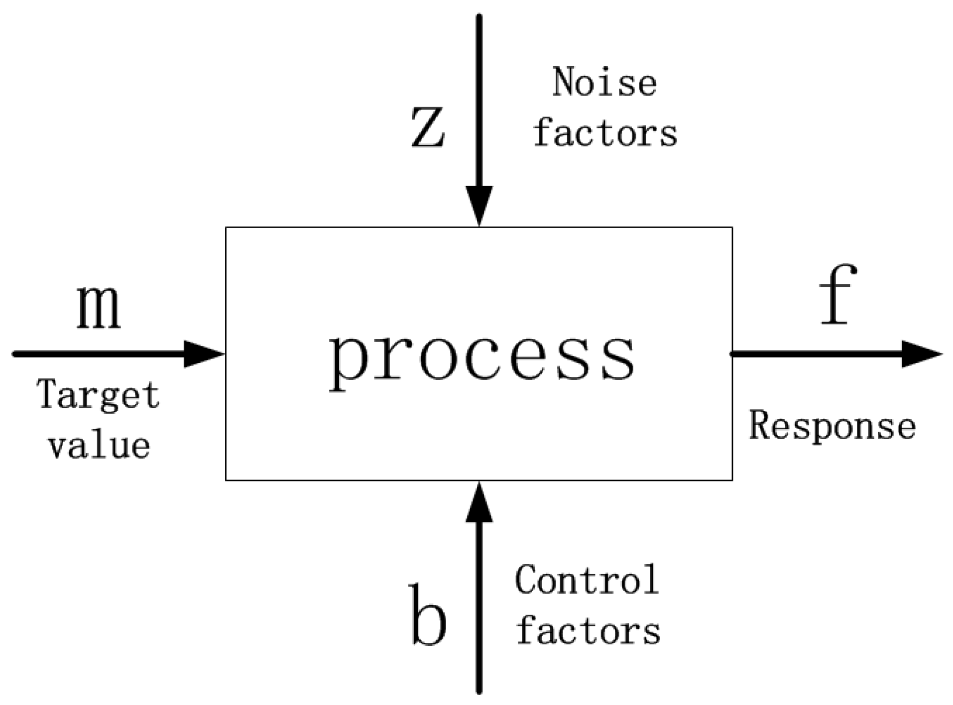
where k is the constant, m is the target value, μ is the mean of f and σ is the standard deviation of f. Figure 1 represents the relation between the factors and the process.
The noise factor is the one that the designer cannot control even though it causes variability, while control factors are design variables. the Taguchi method aims to minimize the loss function Q and optimize the robustness. It has been proved that minimizing loss function is equivalent to maximizing the signal-to-noise ratio when the response with m is referred to as the nominal-the-best type characteristic. The expression of S / N ratios for different characteristic types are listed in Table 2.
Utilizing the design of experiments, a systematic procedure to perform robust design is developed. Generally speaking, first, the orthogonal arrays are utilized to implement experiments. Then from experiments’ results, the S / N ratios are calculated and the optimum setting of control factors is acquired by analyzing the S / N ratios. Finally, with the S / N ratios maintained, a scale factor is selected to set the mean value to the target value.

3. An Integrated Tolerance Theory for the Kinematic Accuracy Analysis of Landing Gear Mechanisms

3.1. Kinematic Accuracy Model Derived from Jacobian–Torsor Model in a Mechanism

The Jacobian–Torsor model uses FE pairs to represent both the dimensions and variations of an assembly. Based on the results sought in the kinematics of a robot, a generic dispersion in an FE pair can be expressed by a set of six virtual joints and coordinate frames.
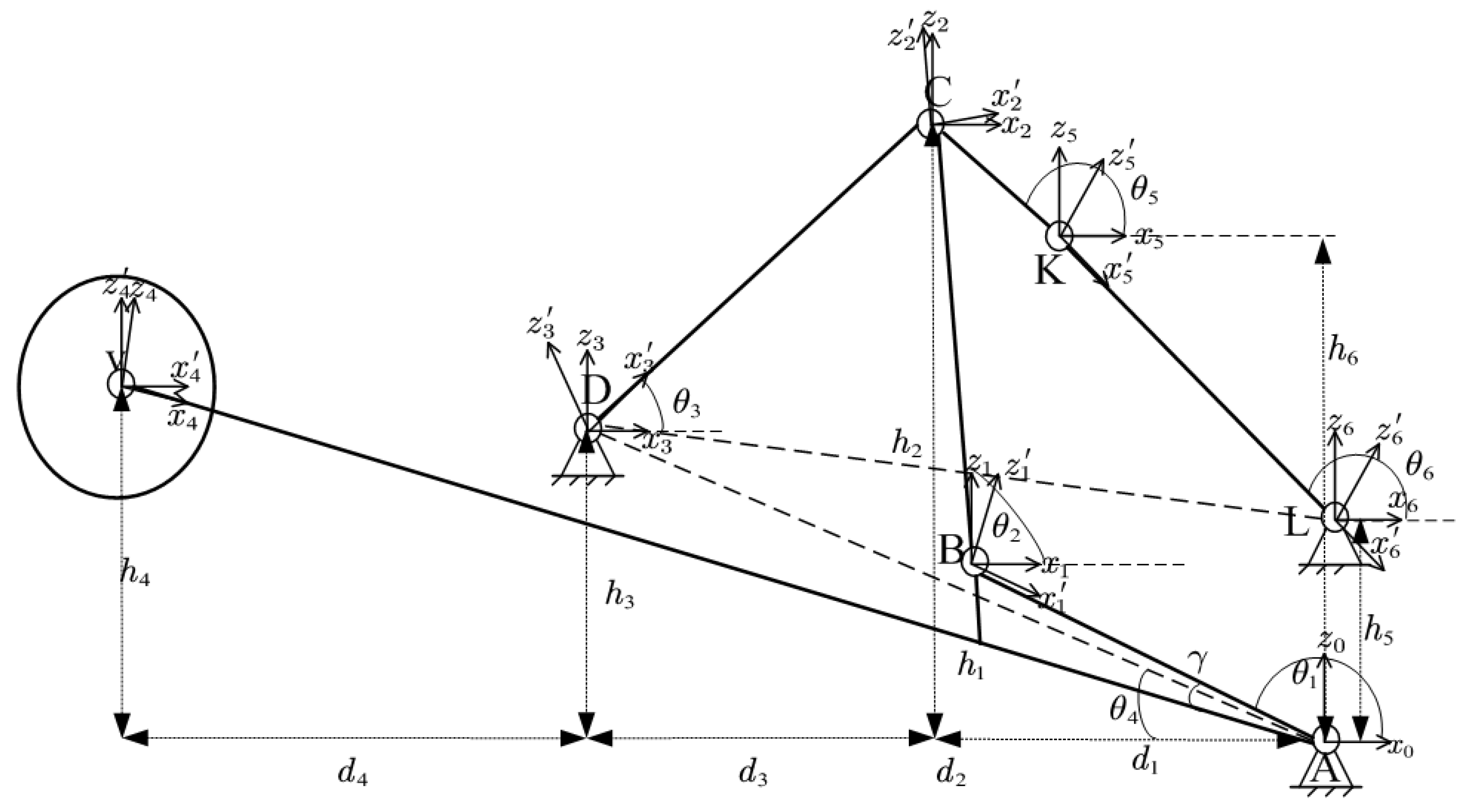
There are six local coordinate frames in an FE pair. (see Figure 2). The transformation matrix from frame 0 to frame 6 can be deduced to be.
T 0 6 = S ( ω 3 4 ) C ( ω 4 5 ) C ( ω 5 6 ) + C ( ω 3 4 ) S ( ω 5 6 ) S ( ω 3 4 ) S ( ω 4 5 ) S ( ω 3 4 ) S ( ω 5 6 ) C ( ω 3 4 ) C ( ω 4 5 ) C ( ω 5 6 ) C ( ω 2 3 ) C ( ω 2 3 ) S ( ω 4 5 ) C ( ω 5 6 ) C ( ω 4 5 ) 0 0 S ( ω 3 4 ) C ( ω 4 5 ) S ( ω 5 6 ) C ( ω 3 4 ) C ( ω 5 6 ) d 2 3 C ( ω 3 4 ) C ( ω 4 5 ) S ( ω 5 6 ) S ( ω 3 4 ) C ( ω 5 6 ) d 1 2 S ( ω 4 5 ) S ( ω 5 6 ) d 0 1 0 1 .
where d i j is translational variable from the frame i to frame j, w i j is rotational variable from the frame i to frame j, S denotes s i n , and C denotes c o s . Similarly, transformation matrices between the other frames of FE pairs can be deduced according to this basic transformation matrix and the following Jacobian matrix J is established based on the transformation matrices between different frames.
The Jacobian–Torsor model expressed in DRF is written as
Δ s Δ α = J 1 J 2 J 3 J 4 J 5 J 6 F E 1 J 6 n 5 J 6 n 4 J 6 n 3 J 6 n 4 J 6 n 5 J 6 n F E n · δ F E i δ F E n
Originally, Jacobian matrix J can be obtained from the overall transform matrix. For small rotational virtual joints, the ith column of the Jacobian matrix J is computed as
J i = z 0 i 1 × ( d 0 n d i 1 ) z 0 i 1 ,
where z 0 i 1 is the third column of T 0 i 1 and d i 1 is the last column of T 0 I 1 . However, In a mechanism, as ( d 0 n d 0 i 1 ) changes with the movement of the kinematic chain, ( d 0 n d 0 i 1 ) can be transformed to f i ( η ) , where η is the input variable of the mechanism. Then,
J i = z 0 i 1 × ( d 0 n d i 1 ) z 0 i 1 = z 0 i 1 × f i ( η ) z 0 i 1 ,
while for small translational virtual joints, there is no contribution to small rotation displacements of the point of interest, and the ith column of the jacobian matrix J i is computed simply as
J i = z 0 i 1 0 ,
Meanwhile, [ δ F E 1 δ F E n ] T are the small deviations of FE pairs, and [ Δ s Δ α ] T is the deviation of the FR. They can be represented as small-displacement screws.
Letting Δ = δ 1 δ 2 δ 3 ϕ 1 ϕ 2 ϕ 3 be a small-displacement screw model, which represents potential variations along and about all three Cartesian axes. Regarding the existence of clearance, when a mechanism moves, FE pairs move, the lengths of FE pairs change, and the small-displacement screw models change as well. For a mechanism, in an FE pair, letting η be the input variable, the projections of lengths and angles, respectively, along and about three axes are
x = f x ( d , η ) , y = f y ( d , η ) , z = f z ( d , η ) ,
θ x = f θ x ( d , η ) , θ y = f θ y ( d , η ) , θ z = f θ z ( d , η ) ,
and then,
Δ x = i = 1 n f x ( d , η ) d i Δ d i , Δ y = i = 1 n f y ( d , η ) d i Δ d i , Δ z = i = 1 n f y ( d , η ) d i Δ d i ,
Δ θ x = i = 1 n f θ x ( d , η ) d i Δ d i , Δ θ y = i = 1 n f θ y ( d , η ) d i Δ d i , Δ θ z = i = 1 n f θ z ( d , η ) d i Δ d i ,
respectively, where Δ x , Δ y , Δ z , Δ θ x , Δ θ y , and Δ θ z are, respectively, small deviations that are functions of the input variables η and Δ d i . As a consequence, the small-displacement screw model of the ith FE pair in the LRF is
Δ F E i = δ 1 δ 2 δ 3 ϕ 1 ϕ 2 ϕ 3 = Δ x Δ y Δ y Δ θ x Δ θ y Δ θ z = i = 1 n f x ( d , η ) d i Δ d i i = 1 n f y ( d , η ) d i Δ d i i = 1 n f z ( d , η ) d i Δ d i i = 1 n f θ x ( d , η ) d i Δ d i i = 1 n f θ y ( d , η ) d i Δ d i i = 1 n f θ z ( d , η ) d i Δ d i
Δ F E i and and the jacobian matrix of a mechanism both change as it moves. For a mechanism which contains n functional elements pairs, kinematic accuracy model in the GRF can be described as
δ 1 δ 2 δ 3 θ 1 θ 2 θ 3 = J 1 J 2 J 6 F E 1 J 6 n 5 J 6 n 4 , J 6 n F E n · Δ F E 1 Δ F E i Δ F E n
here, [ δ 1 δ 2 δ 3 θ 1 θ 2 θ 3 ] T is the small displacement screw model of FR in the GRF. The Δ F E i and J are functions of input variables and tolerances. The clearance between parts is taken as a functional pair and modeled as a small-displacement screw model.

3.2. Analysis of Variance and S / N Ratios for Tolerance Analysis

Robust design involves Analysis of variance (ANOVA) and S / N analysis. ANOVA is a technique for analyzing the way how a variable is affected by different types and combinations of factors. The main parameters of an ANOVA are the Sum of Squared Deviations, Mean Squared Deviations, Contributions, and Confidences. By the analysis, the main factors and their effects are identified. Then, Taguchi analysis is carried out and S / N ratios of control factors are obtained.
S / N ratio is an index of robustness in experiment designs. In other words, A higher S / N ratio is preferred because a high value of S / N ratio implies that the signal is much higher than the uncontrolled noise factors.
After ANOVA (mainly including the Sum of Squared Deviations, Contribution, and Confidence) and S / N analysis, the optimum setting of control factors is determined and a robust tolerance design can be achieved.
The purpose of kinematic accuracy analysis is to find a robust mechanism insensitive to the tolerances and clearances. This coincides with the main ideology of robust design using the Taguchi method. Naturally, the indexes of robust design are considered to be applied in the area of mechanism sensitivity analysis.

3.3. The Integrated Tolerance Analysis Procedure

As described in Section 3.1, six constitute elements exist in a small displacement screw model. Each element for the final functional requirement must be formed as:
δ k = i = 1 n i = 1 6 J i j k δ i j ( k = 1 6 )
Following the concepts in robust design, the ranges of δ i j can be easily controlled by the designer and they can be treated as control factors. The ranges of these tolerances are taken as levels of control factors. Although the kinematic accuracy model is adopted and clearances are taken as functional element pairs, there are still uncountable uncontrollable factors, such as temperature, deformation. Consequently, all other factors which cannot be controlled are noise factors.
For joint clearances in a mechanism, the integrated tolerance analysis procedure is described as follows.
  • Establish the kinematic accuracy model of a mechanism and deduce the propagation function for the FR,
  • According to the experience and engineering handbook, conduct primary tolerance design and analysis,
  • Select control factors and their corresponding levels, and choose an orthogonal array as an experiment matrix,
  • Perform the experiments and calculate S / N ratios,
  • Analyze the S / N ratios, and obtain the optimum setting of control factors,
  • Verify the obtained factors and conduct tolerance redesign and reanalysis.

4. The Tolerance Design and Robust Study for the Joint Clearances of a Landing Gear Retraction Mechanism

In this section, a typical landing gear retraction mechanism is chosen as an example to illustrate the methodology proposed. In Section 4.1, primary tolerance design and analysis are carried out. To decrease the fluctuation of the errors, the integrated theory proposed is used in Section 4.2. In Section 4.3, a revised tolerance design is given, and the analysis completed.
The retracted and extended position of the landing gear is shown in Figure 3. AV is the main struct; OP is the actuator cylinder and serves as the driving component; CD and BC are the drag braces; KL and KC are the lock links; QR is the lock actuator; DE, EF, FG, GH, and HI constitute a linkage mechanism, which connects the hatch door.
When the landing gear is fully retracted and extended, DC, CK, and KL make up the lock mechanism, which maintains the landing gear in the retracted and extended position, respectively. However, the landing gear is not stable when it approaches the retracted and extended position. The problem is strongly related to the kinematic accuracy of the mechanism and the joint clearances are indispensable.
According to the contact theories which are summarized by Johnson, two assumptions must be described before beginning analysis:
  • There is no deformation because of contacts in joints.
  • Contacts between the hole and shaft are supposed to be line contact.

4.1. Primary Clearance Design and Tolerance Analysis of the Mechanism

DC, CB, and AV constitute the main connecting mechanism, while DC, CK, and KL make up the lock mechanism. The simplified diagram is in Figure 4, and the basic parameters are listed in Table 3. The joint clearances of the main connecting and lock mechanism are critical for the kinematic accuracy, and therefore, the tolerance design and robust analysis will be performed next.
Based on the experience and engineering handbook, the tolerances of the components are allocated according to the medium level and they are listed in Table 4.
The kinematic tolerance changes of the landing gear retraction mechanism are along x and z direction, and therefore, δ 1 and δ 3 are the final errors. According to the theory described above, the overall mathematical model is deduced as
δ 1 = r e A · cos θ 1 + Δ A B · cos θ 1 + r e B · cos θ 2 + Δ B C · cos θ 2 + r e C · cos ( π θ 3 ) + Δ C D · cos θ 3 + r e D · cos θ 3 + r e K · cos θ 5 + Δ C K · cos θ 5 + r e L · cos θ 6 + Δ K L · cos θ 6 δ 3 = r e A · sin θ 1 + Δ A B · sin θ 1 + r e B · sin θ 2 + Δ B C · sin θ 2 + r e C · sin ( π θ 3 ) + Δ C D · sin θ 3 + r e D · sin θ 3 + r e K · sin θ 5 + Δ C K · sin θ 5 + r e L · sin θ 6 + Δ K L · sin θ 6 Δ = δ 1 2 + δ 3 2
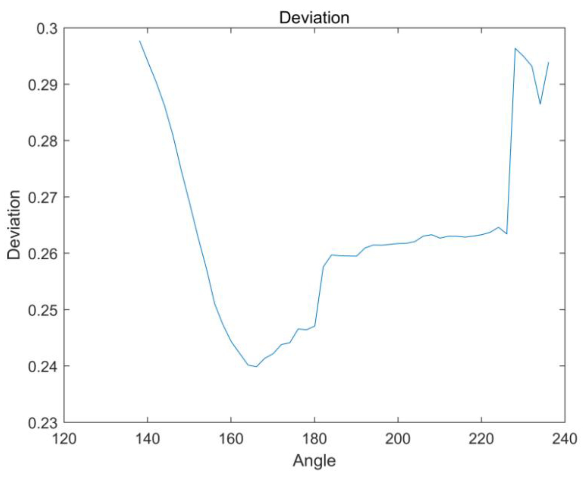
Letting θ change from 133.4° to 233.4°, calculations are performed every 2°. The Monte Carlo method is used in the calculation, the tolerances of the components and joint clearances obey norm distribution as they are shown in Table 3, and the test number is chosen as 100,000. Mean errors for all angles are depicted in Figure 5.
Looking at Figure 4, When the landing gear mechanism retracts or extends, it is apparent that the fluctuation of the errors is comparatively large. The influences of joint clearances are undeniable. In this case, the method proposed can be utilized to reduce the fluctuation range.

4.2. Robust Analysis

The overall mathematical model is Δ = δ 1 2 + δ 3 2 . r e A , r e B , r e C , r e D , r e K , and r e L can be seen as the control factors, their mid-values are corresponding levels as they are shown in Table 5. Letting θ 133.4° to 233.4°, calculations are performed every 10°. The Monte Carlo method is used in the calculation, L 27 ( 3 5 ) is selected as the orthogonal array and shown in Table A1.
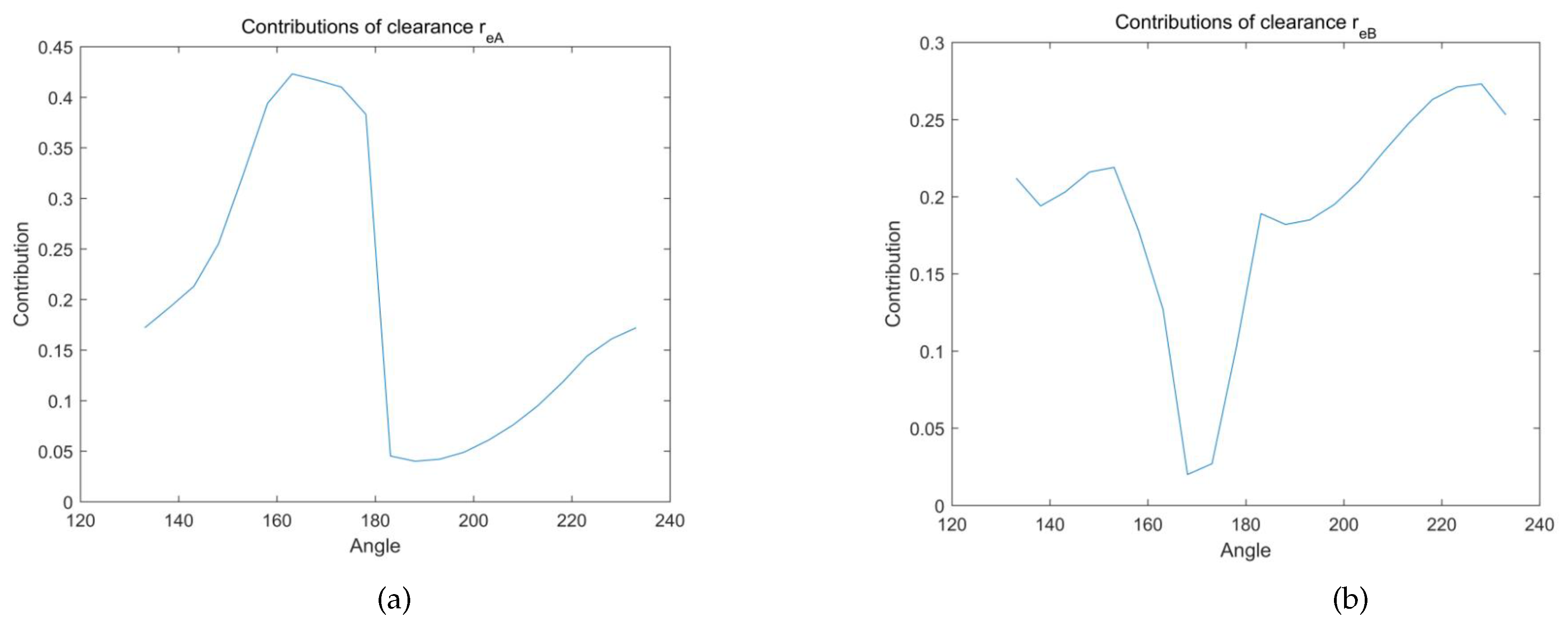
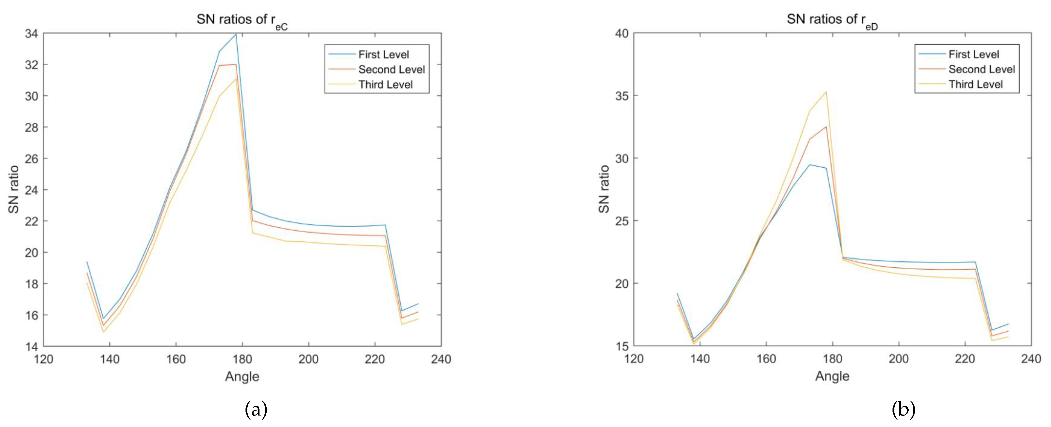
Using Matlab and Minitab, the numerical computation was carried out. For ANVOA analysis, the null hypothesis was: there is no significant effect of a certain joint clearance to the final output results, while the alternative hypothesis was: there is a significant effect of a certain joint clearance to the final output results. The contributions of joint clearances are depicted in Figure 6, Figure 7, Figure 8 and Figure 9; and SN ratios are depicted in Figure 10, Figure 11 and Figure 12.
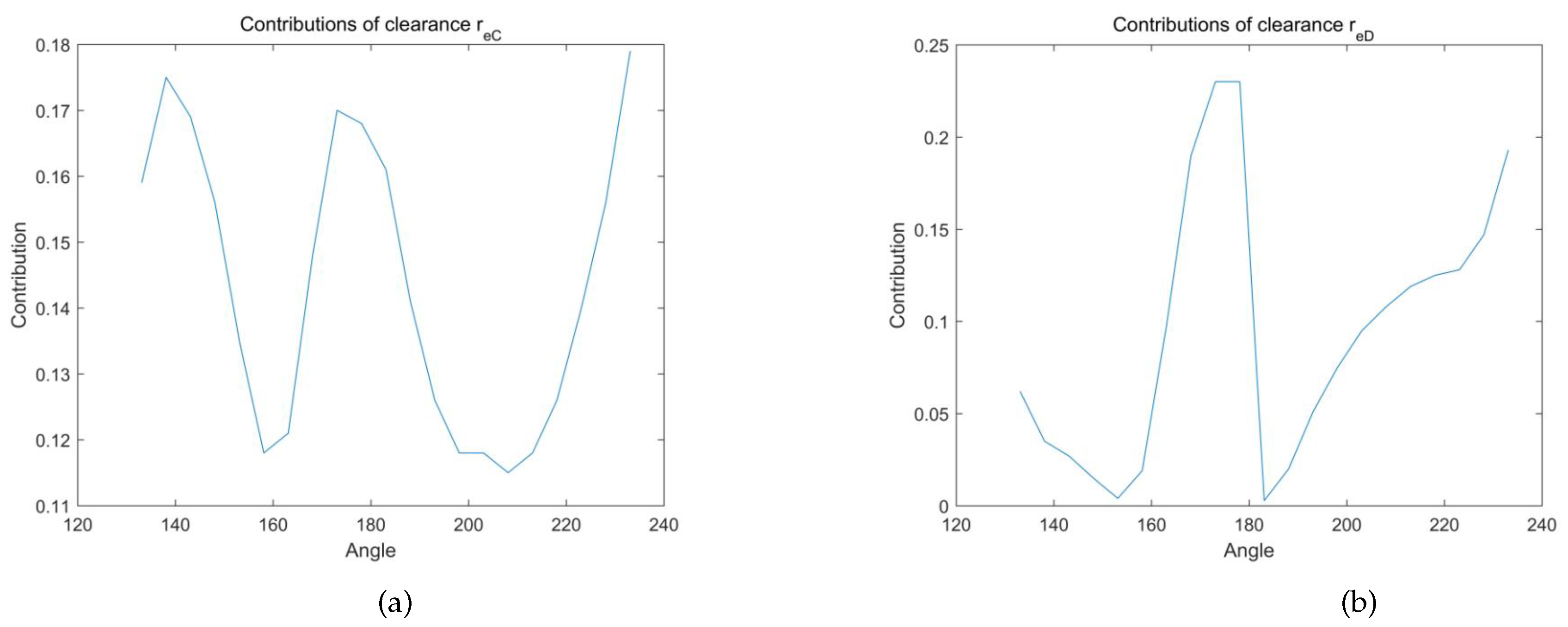
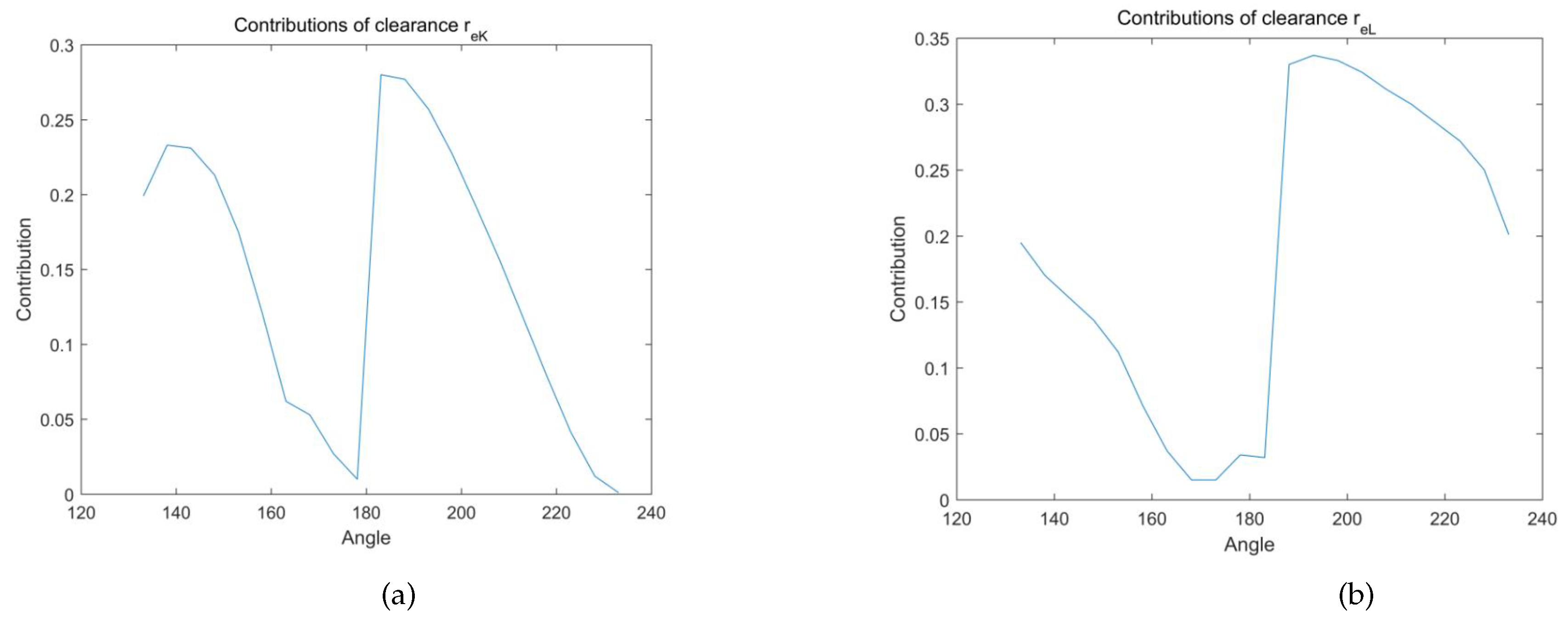
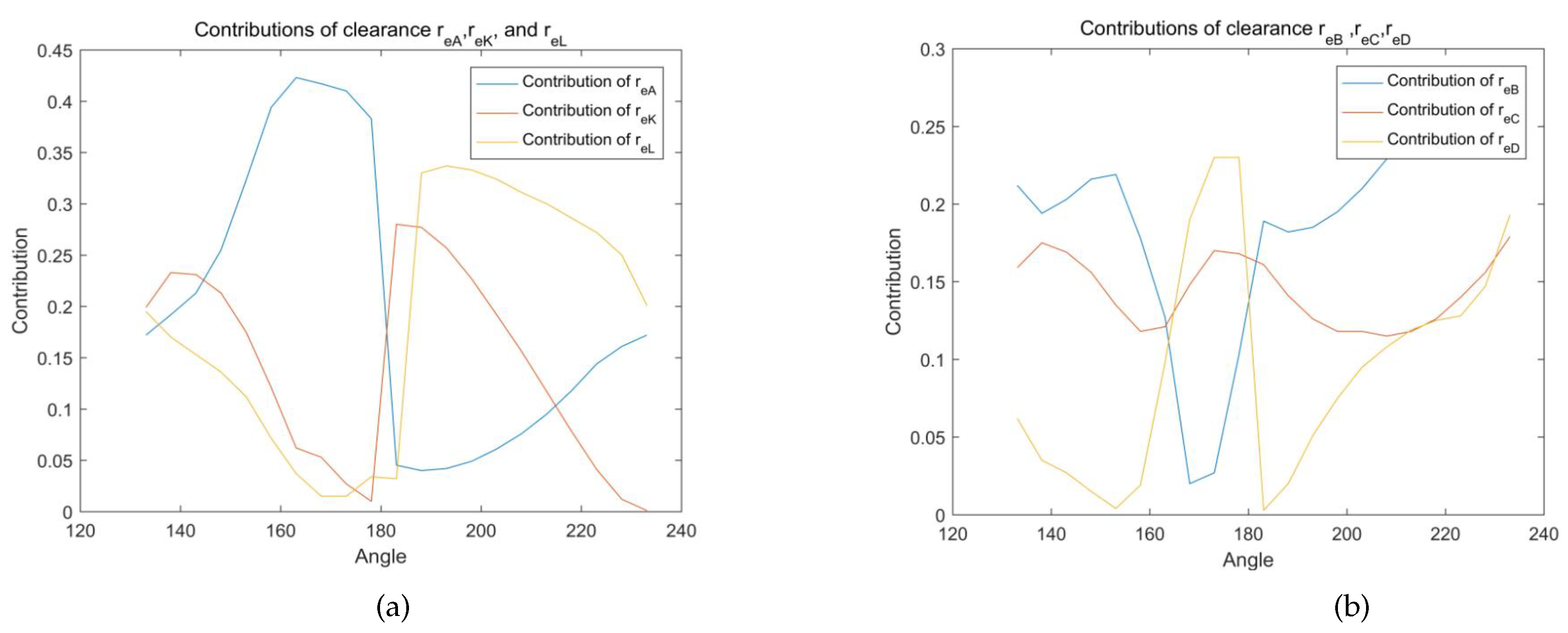
Figure 6, Figure 7, Figure 8 and Figure 9 display the contributions of r e A , r e B , r e C , r e D , r e K , and r e L , and they change as the input variable θ changes. In Figure 6a, when the input variable θ is within the range of 133° 178°, the contribution of r e A increases from 17% to 42%; when θ is 183°, the contribution drops to 4.2%, and then gradually increases again until it reaches 17%. In Figure 6b, the highest contribution of r e B is 28%, and the lowest contribution is 2%; they happen when θ are 163° and 228° respectively. As shown in Figure 7, the contributions of r e C and r e D , change in the range of 12%∼17%, and 0%∼20% respectively. They have one feature in common; that is, during the period 168°∼178°, they both first increase, then decrease. In Figure 8, the tendencies of the two curves are similar. They both decrease first; then during the period of 178°∼183°, suddenly increase; and then decrease again. The ranges of them are within 1% ∼28% and 0%∼34% respectively. In Figure 9, it can be seen that the contributions of r e A , r e K , and r e L are comparatively larger than the other three contributions.
The confidence probabilities of r e A and r e C are much less than 5%, therefore, the null hypothesis is denied. They have significant effects on the final results. For r e B , r e D , r e K , and r e L , when θ is within the range of 178°∼183°, there is a tendency to accept the null hypothesis; however, mostly their contributions are less than 5%, and the null hypothesis cannot be accepted yet.
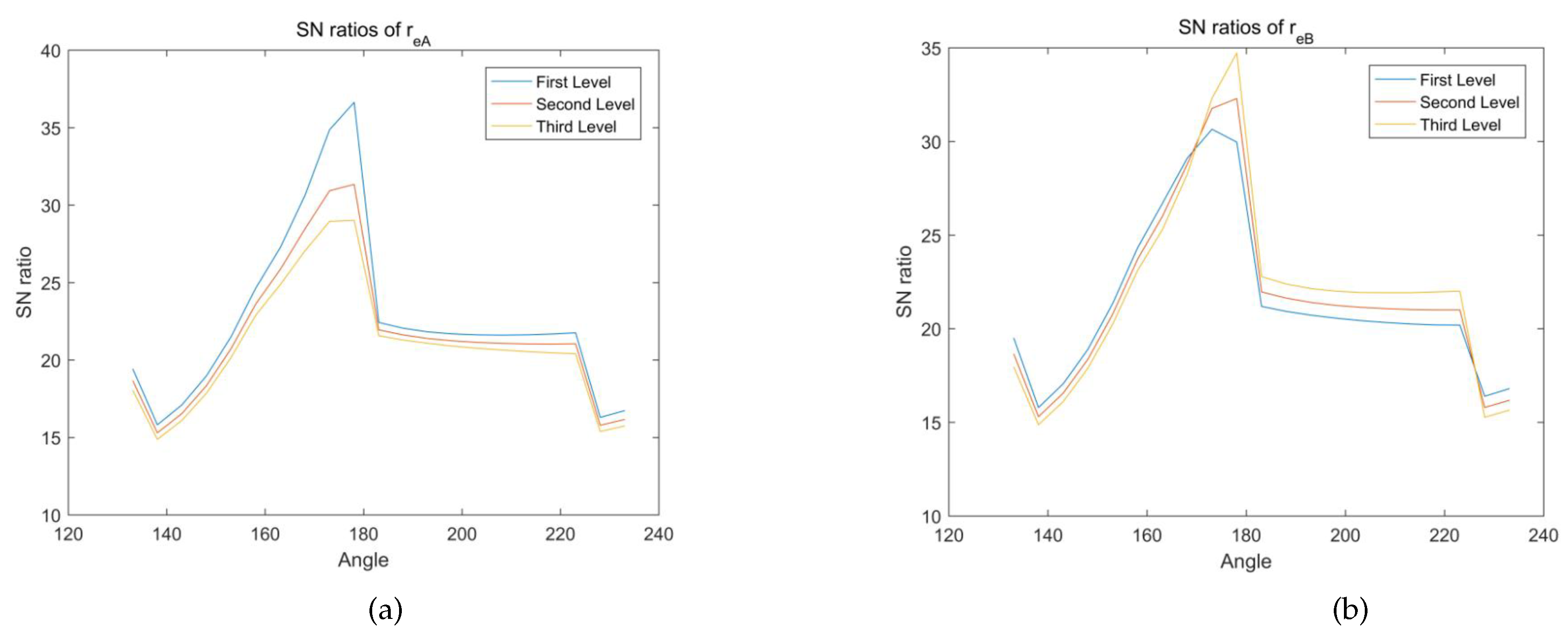
Figure 10, Figure 11 and Figure 12 provide S / N ratios of all control factors. In general, the tendencies of the curves are similar. As the input variable θ approaches 178°, the S / N ratios gradually increase, then they begin to decrease. When θ is within the range of 163°∼183°, the ranges of S / N ratios become larger until they reach the largest ones during the processes. However, the effects of the six control factors are different.
A significant correlation can be observed in Figure 10, that is, the S / N ratios of the first level are larger than the second level, and the second larger than the third. The finding indicates that the size of r e A has a negative influence on the final results, and output deviation decreases as r e A increases. The indication holds for r e C , r e K , r e L as well, as it can be seen from Figure 11 and Figure 12. For r e B and r e D , they have positive influences when θ is during the periods of 168°∼223° and 163°∼183° respectively. Excluding this, they have negative influences as well.
Based on the discussions above, basic findings and suggestions are summarized as follows.
  • All six clearances have significant effects on final results, however, different clearances have different effects.
  • When the input variable is within the range of 153°∼223°, fluctuations exist for six curves of the contributions, indicating that the effects of six clearances can not be overlooked.
  • Referring to the results, the order of the effects can be given as: r e A > r e L > r e B > r e K > r e C > r e D . r e A , r e C , r e K , and r e L have negative effects on final results, and output deviation decrease as they increase. For most of the time, r e B and r e B have negative influences. However, when θ is during the periods of 168°∼223° and 163°∼183° respectively, they have positive influences.

4.3. Modified Tolerance Design for Joint Clearances

Given the observations in Section 4.2, modified tolerance design parameters are given in Table 6.
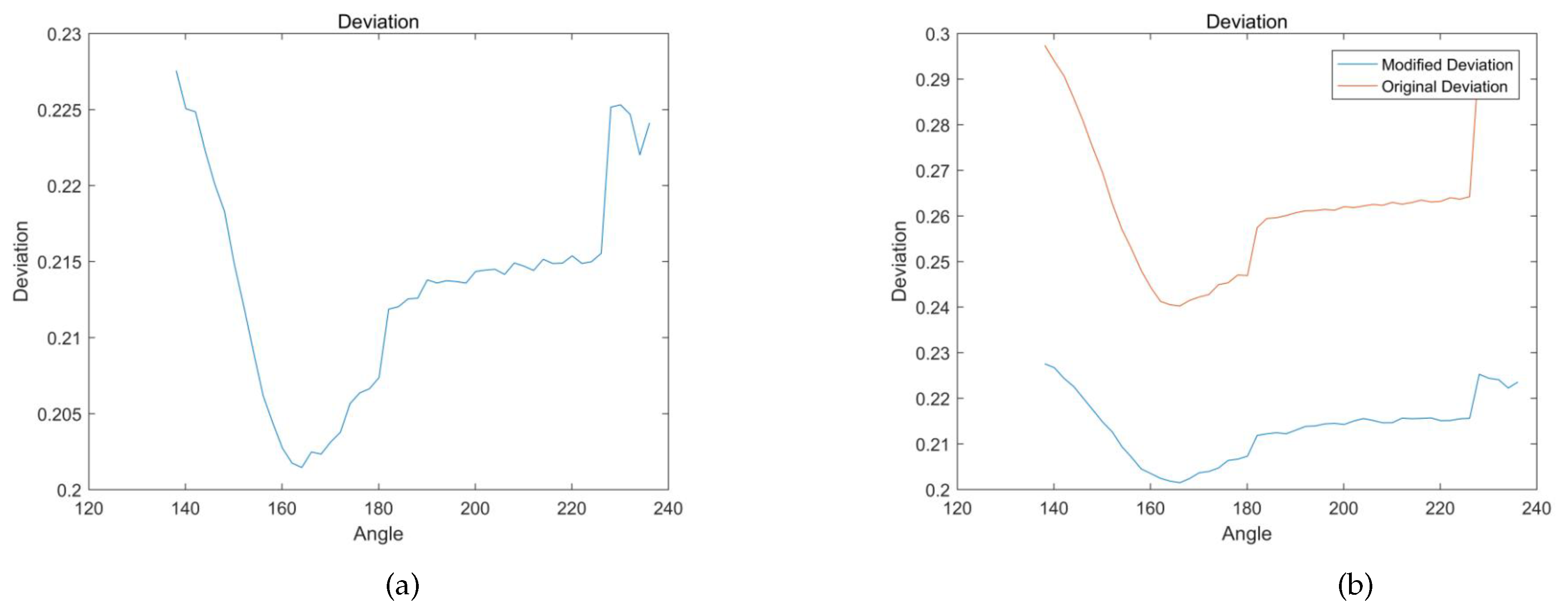
With the input variable increasing from 133.4° to 234.3°, calculations are performed every 2°. Monte Carlo method is used, and the test number is 100,000. Modified mean deviations for all angles are depicted in Figure 12. The comparison is shown in Figure 13.
As can be seen from the Figure 12 and Figure 13, modified deviations are reduced by about 23%. The reason is that the internal tendencies are easily observed through the robust analysis of tolerances, which help the designers to make proper resolutions. This rather reassuring result indicates that the theories proposed in previous sections can be used to study the clearance effects and assure the robustness of a mechanism.

5. Conclusions

The main purpose of this study was to form an integrated theory for the clearance analysis of landing gear retraction mechanisms. Major contributions and comments are summarized as follows:
  • A new integrated theory composed of tolerance design and robust analysis was presented. The Jacobian tolerance theories were adopted to deduce the kinematic accuracy model, while robust theories are used to analyze the tolerance effects of a mechanism. The procedures of the theory are also given.
  • A typical landing gear retraction mechanism was taken as a case to study the joint clearance effects. Using the presented theory, joint clearances were seen as tolerances. Through the procedures of tolerance design, robust analysis, and tolerance redesign, final results showed that modified deviations of the landing gear retraction mechanism were significantly reduced, which suggests that the integrated theory presented is a valid way to estimate the influences of joint clearances and keep the robustness of a mechanism.
  • The study has have found that the inner tendencies of joint clearances could be observed. This finding provides designers assistance for sound decisions and researchers’ insights for future studies on joint clearances. According to the finding and the results of the study case, the designers are planning to modify the tolerance parameters to obtain a more robust mechanism and further research will continue.
  • Regarding landing gear retraction mechanism, the integrated theory and the study presented contribute in several ways to our understanding of tolerance design and robust analysis. This is the first study to integrate tolerance and robust theories and analyze the clearance effects on landing gear kinematic accuracy. The theory and the findings will be of great use for landing gears in the future design.
  • The jacobian model has the advantage of simplicity and clarity. This is also the first study to use the jacobian model for the tolerance analysis of the landing gear mechanism. Future studies regarding the role of the jacobian model are strongly recommended.

Author Contributions

Conceptualization: H.N., X.W., L.Z.; Methodology: L.Z.; Validation: H.N., X.W.; Formal analysis: L.Z.; Investigation:H.N., X.W., L.Z.; Resources: H.N., X.W., L.Z.; Data curation: L.Z.; Writing original draft: L.Z.; Writing review & editing: L.Z., H.N., X.W.; Visualization: H.N., X.W.; Supervision: H.N., X.W.; Project administration: H.N., X.W., L.Z.; Funding acquisition: H.N., X.W. All authors have read and agreed to the published version of the manuscript.

Funding

This work described in this paper is supported in part by The Fundamental Research Funds for the Central Universities (under Grant No.NF2018001), and in part by National Defense Outstanding Youth Science Foundation (under Grant No. 2018-JCJQ-ZQ-053).

Acknowledgments

The authors would like to thank the anonymous reviewers, associate editor, and editor for their valuable and constructive comments and suggestions.

Conflicts of Interest

The authors declare no conflict of interest.

Abbreviations

The following abbreviations are used in this manuscript:
FEFunctional element
FRFunctional requirement
FE pairFunctional element pair
GRFGlobal reference frame
LRFLocal reference frame

Appendix A

The orthogonal array required in Section 4.2 is shown below.
Table A1. Slider-crank parameters.
Experiments r eA r eB r eC r eD r eK r eL
10.0270.0270.0270.0270.0270.027
20.0270.0270.0270.0270.0370.037
30.0270.0270.0270.0270.0470.047
40.0270.0370.0370.0370.0270.027
50.0270.0370.0370.0370.0370.037
60.0270.0370.0370.0370.0470.047
70.0270.0470.0470.0470.0270.027
80.0270.0470.0470.0470.0370.037
90.0270.0470.0470.0470.0470.047
100.0370.0270.0370.0470.0270.037
110.0370.0270.0370.0470.0370.047
120.0370.0270.0370.0470.0470.027
130.0370.0370.0470.0270.0270.037
140.0370.0370.0470.0270.0370.047
150.0370.0370.0470.0270.0470.027
160.0370.0470.0270.0370.0270.037
170.0370.0470.0270.0370.0370.047
180.0370.0470.0270.0370.0470.027
190.0470.0270.0470.0370.0270.047
200.0470.0270.0470.0370.0370.027
210.0470.0270.0470.0370.0470.037
220.0470.0370.0270.0470.0270.047
230.0470.0370.0270.0470.0370.027
240.0470.0370.0270.0470.0470.037
250.0470.0470.0370.0270.0270.047
260.0470.0470.0370.0270.0370.027
270.0470.0470.0370.0270.0470.037

References

  1. Committee of Aircraft. Aircraft Design Manual Book 14: Taking-off and Landing Devices Design; Aviation Industry Press: Beijing, China, 2002. [Google Scholar]
  2. Currey, N. Aircraft Landing Gear Design: Principle and Practice; AIAA: Washington, DC, USA, 1988. [Google Scholar]
  3. Chen, B. Aircraft Manufacturing coordination Accuracy and Tolerance Allocation; Aviation Industry Press: Beijing, China, 1987. [Google Scholar]
  4. Laperrière, L.; Lafond, P. Tolerance Analysis And Synthesis Using Virtual Joints; Springer: Dordrecht, The Netherlands, 1999. [Google Scholar]
  5. Laperrière, L.; ElMaraghy, H.A. Tolerance Analysis and Synthesis Using Jacobian Transforms. CIRP Ann. 2000, 49, 359–362. [Google Scholar] [CrossRef]
  6. Lafond, P.; Laperriere, L. Jacobian-based modeling of dispersions affecting pre-defined functional requirements of mechanical assemblies. In Proceedings of the 1999 IEEE International Symposium on Assembly and Task Planning (ISATP’99) (Cat.No.99TH8470), Porto, Portugal, 24 July 1999; pp. 20–25. [Google Scholar]
  7. Desrochers, A.; Riviere, A. A matrix approach to the representation of tolerance zones and clearances. Int. J. Adv. Manuf. Technol. 1998, 13, 630–636. [Google Scholar] [CrossRef]
  8. Chase, K.W.; Jinsong, G.; Magleby, S.P. Generalized 3D tolerance analysis of mechanical assemblies with small kinematic adjustments. IIE Trans. 2000, 30, 367–377. [Google Scholar]
  9. Desrochers, A.; Clement, A. A dimensioning and tolerancing assistance model for CAD/CAM systems. Int. J. Adv. Manuf. Technol. 2000, 9, 352–361. [Google Scholar] [CrossRef]
  10. Laperrière, L.; Ghie, W.; Desrochers, A. Statistical and Deterministic Tolerance Analysis and Synthesis Using a Unified Jacobian–Torsor Model. CIRP Ann. 2002, 51, 417–420. [Google Scholar] [CrossRef]
  11. Frisoli, A.; Solazzi, M.; Pellegrinetti, D.; Bergamasco, M. A new screw theory method for the estimation of position accuracy in spatial parallel manipulators with revolute joint clearances. Mech. Mach. Theory 2011, 46, 1929–1949. [Google Scholar] [CrossRef]
  12. Ghie, W.; Laperrière, L.; Desrochers, A. Statistical tolerance analysis using the unified Jacobian–Torsor model. Int. J. Prod. Res. 2009, 48, 4609–4630. [Google Scholar] [CrossRef]
  13. Franciosa, P.; Gerbino, S.; Patalano, S. Variational modeling and assembly constraints in tolerance analysis of rigid part assemblies: Planar and cylindrical features. Int. J. Adv. Manuf. Technol. 2009, 49, 239–251. [Google Scholar]
  14. Asante, J.N. A small displacement torsor model for tolerance analysis in a workpiece-fixture assembly. Proc. Inst. Mech. Eng. Part B J. Eng. Manuf. 2009, 223, 1005–1020. [Google Scholar] [CrossRef]
  15. Desrochers, A.; Ghie, W.; Laperriere, L. Application of a unified Jacobian–Torsor model for tolerance analysis. J. Comput. Inf. Sci. Eng. 2003, 3, 2–14. [Google Scholar] [CrossRef]
  16. Adams, J.D.; Whitney, D.E. Application of screw theory to constraint analysis of mechanical assemblies joined by features. J. Mech. Des. 2001, 123, 26–32. [Google Scholar] [CrossRef]
  17. Tobon, S.A.; Teissandier, D.; Delos, V. Applying screw theory for summing sets of constraints in geometric tolerancing. Mech. Mach. Theory 2017, 112, 255–271. [Google Scholar] [CrossRef]
  18. Li, H.; Zhu, H.; Zhou, X.; Li, P.; Yu, Z. A new computer-aided tolerance analysis and optimization framework for assembling processes using DP-SDT theory. Int. J. Adv. Manuf. Technol. 2016, 86, 1299–1310. [Google Scholar] [CrossRef]
  19. Jin, S.; Chen, H.; Li, Z.M.; Lai, X.M. A small displacement torsor model for 3D tolerance analysis of conical structures. Proc. Inst. Mech. Eng. Part C J. Mech. Eng. Sci. 2015, 229, 2514–2523. [Google Scholar] [CrossRef]
  20. Zuo, X.; Li, B.; Yang, J.; Jiang, X. Application of the Jacobian–torsor theory into error propagation analysis for machining processes. Int. J. Adv. Manuf. Technol. 2013, 69, 1557–1568. [Google Scholar] [CrossRef]
  21. Chen, H.; Jin, S.; Li, Z.M.; Lai, X.M. A solution of partial parallel connections for the unified Jacobian–Torsor model. Mech. Mach. Theory 2015, 91, 39–49. [Google Scholar] [CrossRef]
  22. Chen, H.; Jin, S.; Li, Z.; Lai, X. A modified method of the unified Jacobian–Torsor model for tolerance analysis and allocation. Int. J. Precis. Eng. Manuf. 2015, 16, 1789–1800. [Google Scholar] [CrossRef]
  23. Chen, H.; Jin, S.; Li, Z.M.; Lai, X.M. A comprehensive study of three dimensional tolerance analysis methods. Comput.-Aided Des. 2014, 53, 1–13. [Google Scholar] [CrossRef]
  24. Zhou, X.; Li, H.; Zhu, H.P. A novel kinematic accuracy analysis method for a mechanical assembly based on DP-SDT theory. Int. J. Adv. Manuf. Technol. 2018, 94, 4301–4315. [Google Scholar] [CrossRef]
  25. Taguchi, G. Systems of Experimental Design Kraus International; Kraus International Pub & American Supplier Institute: New York, NY, USA, 1987. [Google Scholar]
  26. Erkaya, S.; Uzmay, I. Determining link parameters using genetic algorithm in mechanisms with joint clearance. Mech. Mach. Theory 2009, 44, 222–234. [Google Scholar] [CrossRef]
  27. Stander, N.; Craig, K.J. On the robustness of a simple domain reduction scheme for simulation-based optimization. Eng. Comput. 2002, 19, 431–450. [Google Scholar] [CrossRef] [Green Version]
  28. Lee, K.H.; Park, G.J. Robust optimization in discrete design space for constrained problems. Aiaa J. 2002, 40, 774–780. [Google Scholar] [CrossRef]
  29. Zhu, J.M.; Ting, K.L. Performance distribution analysis and robust design. J. Mech. Des. 2001, 123, 11–17. [Google Scholar] [CrossRef]
  30. Gong, C.; Kao, I. Design for accuracy and repeatability for robots using Taguchi methods. Concurrent. Eng. Res. A 1997, 5, 263–277. [Google Scholar]
  31. Ting, K.; Long, Y. Performance Quality and Tolerance Sensitivity of Mechanisms. J. Mech. Des. 1996, 118, 144–150. [Google Scholar] [CrossRef]
  32. Tsui, K.L. An overview of Taguchi method and newly developed statistical methods for robust design. IIE Trans. 1992, 24, 44–57. [Google Scholar] [CrossRef]
  33. Caro, S.; Bennis, F.; Wenger, P. Tolerance synthesis of mechanisms: A robust design approach. J. Mech. Des. 2005, 127, 86–94. [Google Scholar] [CrossRef] [Green Version]
  34. Rout, B.K.; Mittal, R.K. Tolerance design of robot parameters using Taguchi method. Mech. Syst. Signal Process. 2006, 20, 1832–1852. [Google Scholar] [CrossRef]
  35. Dua, X.P.; Venigella, P.K.; Liu, D.S. Robust mechanism synthesis with random and interval variables. Mech. Mach. Theory 2009, 44, 1321–1337. [Google Scholar] [CrossRef]
  36. Luo, K.; Wang, J.G.; Du, X.P. Robust mechanism synthesis with truncated dimension variables and interval clearance variables. Mech. Mach. Theory 2012, 57, 71–83. [Google Scholar] [CrossRef]
  37. Huang, X.Z.; Zhang, Y.M. Robust tolerance design for function generation mechanisms with joint clearances. Mech. Mach. Theory 2010, 45, 1286–1297. [Google Scholar] [CrossRef]
  38. Huang, X.Z.; Zhang, Y.M.; Lu, H.; Tang, L.; Li, H. Tolerance Design for Four-Bar Function Generating Mechanisms with Joint Clearances Using Taguchi Method; Trans Tech Publications Ltd: Stafa-Zurich, Switzerland, 2010. [Google Scholar]
  39. Armillotta, A. A static analogy for 2D tolerance analysis. Assem. Autom. 2014, 34, 182–191. [Google Scholar] [CrossRef] [Green Version]
  40. Park, G.J.; Lee, T.H.; Lee, K.H.; Hwang, K.H. Robust design: An overview. Aiaa J. 2006, 44, 181–191. [Google Scholar] [CrossRef]
Sample Availability: Samples of the paper are available from the authors.
Figure 1. Robust Design.
Applsci 10 04856 g001
Figure 2. Virtual joints and coordinate frames in an FE pair.
Applsci 10 04856 g002
Figure 3. The landing gear retraction mechanism: (a) the retracted position; (b) the extended position.
Applsci 10 04856 g003
Figure 4. The main connecting and lock mechanism.
Applsci 10 04856 g004
Figure 5. Original deviations for the primary tolerance design.
Applsci 10 04856 g005
Figure 6. (a) The contributions of r e A ; (b) The contributions of r e B .
Applsci 10 04856 g006
Figure 7. (a) The contributions of r e C ; (b) The contributions of r e D .
Applsci 10 04856 g007
Figure 8. (a) The contributions of r e K ; (b) The contributions of r e L .
Applsci 10 04856 g008
Figure 9. (a) The contributions of r e A , r e B , and r e C ; (b) The contributions of r e D , r e K , and r e L .
Applsci 10 04856 g009
Figure 10. (a) The SN ratios of r e A ; (b) The SN ratios of r e B .
Applsci 10 04856 g010
Figure 11. (a) The SN ratios of r e C ; (b) The SN ratios of r e D .
Applsci 10 04856 g011
Figure 12. (a) The SN ratios of r e K ; (b) The SN ratios of r e L .
Applsci 10 04856 g012
Figure 13. (a) The modified deviations; (b) The comparison of original and modified deviations.
Applsci 10 04856 g013
Table 1. The basic concepts of the Jacobian model.
ParameterDefinition
Functional element (FE):Point, curve, or surface that belongs to a part in the assembly. A FE can be real, e.g., the plane surface of a block, or constructed, e.g., the axis of a cylinder or a median plane.
Functional requirement (FR):An important condition to be satisfied between two FEs on different parts, e.g., a fitting condition.
Virtual jointsFor tolerancing purposes, we associate coordinate frames to the toleranced FE in a pair, assuming there exists a set of virtual joints that can make the toleranced FE of the pair “move” relative to the other FE of the pair, to simulate manufacturing inaccuracies.
Functional element pair (FE pair)Two FES on different parts or on the same part; includes a kinematic pair and internal pair.
small-displacement screw modelAn expression which contains potential variations along and about all three Cartesian axes.
Global reference frame (GRF)Frame in which the functional requirement and total dimensional chain is established.
Local reference frame (LRF)Frame in which each functional element pair is established.
Table 2. S / N ratios for different characteristic types.
Characteristic Type S / N Ratios
Nominal the bestWith scale factor η = 10 log ( μ 2 / σ 2 )
With adjustment factor η = 10 log ( σ 2 )
Smaller the better η = 10 log [ 1 n i = 1 n y i 2 ]
Larger the better η = 10 log [ 1 n i = 1 n 1 y i 2 ]
Table 3. Slider-crank parameters.
ComponentsLength(mm)AngleScope
AB451.77 θ 1 133.14∼234.30 (input variable)
BC315.8 θ 2 86.257∼62.389
CD465 θ 3 43.481∼−62.389
AD704.89 θ 4 152.544
AV1334.437 θ 5 24.203
KL305 θ 6 122.004∼−141.98
CK195 θ 7 122.004∼−141.98
LD615.359 θ 8 9.453
Table 4. Primary tolerance design parameters.
ComponentsTolerances (mm)
Δ A B Δ A B ( 0 , 0 . 133 2 )
Δ B C Δ B C ( 0 , 0 . 083 2 )
Δ C D Δ C D ( 0 , 0 . 133 2 )
Δ C K Δ C K ( 0 , 0 . 083 2 )
Δ K L Δ K L ( 0 , 0 . 083 2 )
r e A r e A ( 0.047 , 0 . 00283 2 )
r e B r e B ( 0 , 0385 , 0 . 00242 2 )
r e C r e C ( 0.0385 , 0 . 00242 2 )
r e D r e D ( 0.047 , 0 . 00283 2 )
r e K r e K ( 0.0385 , 0 . 00242 2 )
r e L r e L ( 0.0385 , 0 . 00242 2 )
Table 5. Tolerances and experiment levels.
ComponentsTolerances (mm)
r e A Level 1: r e A ( 0.027 , 0 . 00283 2 ) (rough)
Level 2: r e A ( 0.037 , 0 . 00283 2 ) (medium)
Level 3: r e A ( 0.047 , 0 . 00283 2 ) (precise)
r e B Level 1: r e B ( 0.027 , 0 . 00283 2 ) (rough)
Level 2: r e B ( 0.037 , 0 . 00283 2 ) (medium)
Level 3: r e B ( 0.047 , 0 . 00283 2 ) (precise)
r e C Level 1: r e C ( 0.027 , 0 . 00283 2 ) (rough)
Level 2: r e C ( 0.037 , 0 . 00283 2 ) (medium)
Level 3: r e C ( 0.047 , 0 . 00283 2 ) (precise)
r e D Level 1: r e D ( 0.027 , 0 . 00283 2 ) (rough)
Level 2: r e D ( 0.037 , 0 . 00283 2 ) (medium)
Level 3: r e D ( 0.047 , 0 . 00283 2 ) (precise)
r e K Level 1: r e K ( 0.027 , 0 . 00283 2 ) (rough)
Level 2: r e K ( 0.037 , 0 . 00283 2 ) (medium)
Level 3: r e K ( 0.047 , 0 . 00283 2 ) (precise)
r e L Level 1: r e L ( 0.027 , 0 . 00283 2 ) (rough)
Level 2: r e L ( 0.037 , 0 . 00283 2 ) (medium)
Level 3: r e L ( 0.047 , 0 . 00283 2 ) (precise)
Table 6. Primary tolerance design parameters.
ComponentsTolerances (mm)
Δ A B Δ A B ( 0 , 0 . 133 2 )
Δ B C Δ B C ( 0 , 0 . 083 2 )
Δ C D Δ C D ( 0 , 0 . 133 2 )
Δ C K Δ C K ( 0 , 0 . 083 2 )
Δ K L Δ K L ( 0 , 0 . 083 2 )
r e A r e A ( 0.024 , 0 . 00283 2 )
r e B r e B ( 0 , 0205 , 0 . 00242 2 )
r e C r e C ( 0.0205 , 0 . 00242 2 )
r e D r e D ( 0.024 , 0 . 00283 2 )
r e K r e K ( 0.0205 , 0 . 00242 2 )
r e L r e L ( 0.0205 , 0 . 00242 2 )