A Deep Learning Method for Short-Term Dynamic Positioning Load Forecasting in Maritime Microgrids

Featured Application

Application of deep learning techniques to dynamic positioning in maritime microgrids for power management system.

Abstract

The dynamic positioning (DP) system is a progressive technology, which is used in marine vessels and maritime structures. To keep the ship position from displacement in operation mode, its thrusters are used automatically to control and stabilize the position and heading of vessels. Hence, the DP load forecasting is already an essential part of DP vessels, which the DP power demand from the power management system (PMS) for thrusting depends on weather conditions. Furthermore, the PMS is used to control power generation, and prevent power failure, limitation. To perform station keeping of vessels by DPS in environmental changes such as wind, waves, capacity, and reliability of the power generators. Hence, a lack of power may lead to lower DP performance, loss of power, and position, which is called shutdown. Therefore, precise DP power demand prediction for maintaining the vessel position can provide the PMS with sufficient information for better performance in a complex decision-making process for the DP vessel. In this paper, the concept of deep learning techniques is introduced into DPS for DP load forecasting. A Levenberg–Marquardt algorithm based on a nonlinear recurrent neural network is employed in this paper for predicting thrusters’ power consumption in sea state variations due to challenges in power generation with the relative degree of accuracy by combining weather parameter dependencies as environmental disturbances. The proposed method evaluates with three traditional forecasting methods through a set of practical real-time DP load and weather parametric data. Numerical analysis has shown that with the proposed method, the future DP load behavior can be predicted more accurately than that obtained from the traditional methods, which greatly assists in operation and planning of power system to maintain system stability, security, reliability, and economics.

1. Introduction

Operation in deep waters is one of the most challenging in marine industries due to the risk of maneuvering in sea conditions. To avoid using anchor chains, the speed and position of vessels must be counteracted to sea disorders such as waves, wind, and their directions continuously. For establishing the vessel location and headline automatically, vessels are equipped by the dynamic positioning system (DPS), propellers, thrusters [1].

The DPS was first used in the 1960s to control the movement of ships in three horizontal degrees of freedom (HDOF), including sway, surge, and yaw. Where proportional-integral-derivative (PID) controllers were applied in DPS with a low-pass filter control system. The PID control system changed the phase insufficiently, which caused the instability of the system [2]. Hence, Balchen et al. suggested Kalman filtering methods, randomized optimal control theory, and more progressive control techniques to improve the DPS efficiency on ships maneuvering. This was revealed in the theory of kinematic equations [3,4,5,6,7]. On the other hand, the results showed that the movement equations are linear at many predefined constant heading angles in HDOF and the stability of DPS couldn’t be guaranteed. The study in [8] proposed the non-linear control technique based on the backstepping method, where sea disturbances are considered. Hence, the environmental disturbances affected by wind and waves cannot be neglected. Consequently, an inactive non-linear observer was recommended, which consists of an estimate for the low-frequency station bias to measure the speed of the ship during displacement and a wave filter to reduce the number of setting parameters [9]. The performance of the method for designing a proportional-differential (PD) with control law for evaluating the DPS output feedback is shown in [10]. In this evaluation with a ship model, the filter supervisor eliminates noises from the measurement of the position speed of the ship by applying a PD controller that changes gradually because of environmental variations. To decrease the deviation of vessels station from the set point while ecological disturbances cause unexpected sudden changes of position, an adaptive control technique is developed to approximate nonlinear DPS parameters with fuzzy logic theory or neural network (NN) in [11,12,13,14,15,16,17,18,19,20]. As a result, an adaptive NN based on a fuzzy inference system is proposed in [21,22,23], which encloses a fuzzy logic to adapt the NN weights for the period of learning procedure by using fuzzy rules. And so, the control parameters adjust automatically by applying the NN based fuzzy logic rules. In the proposed method, due to time-saving concerns, the mathematical model is not considered by the NN controller. To give emphasis to the necessity for further research, the study in [24,25,26,27,28,29] presented a combined control method, and performance techniques in DP ships under slow to heavy sea conditions are presented, where the non-linear controller was used as an autonomous scale to control the switching to prevent instability and shutdown of the system.

To increase control performance, model predictive control (MPC) is represented in [30,31,32,33,34,35], which can be mathematically executed by a highly precise control method using linear models of the dynamic plant. Hence, MPC simulates the future movement of the ship by using previous control to predict appropriate control output responses, which performed constraints on both input and output variables to estimate the distortion effect on future procedure evolution. Therefore, the prediction model includes abilities in the optimization method to approximate the dynamic response of vessels over a specified time horizon.

On the other hand, depending on the proposed controllers’ nature, the control methods do not react quickly to sudden changes in environmental forces such as wind blows, unless the position predictor can recognize and take timely proper actions. To keep the vessel in the calm to extremely high sea state, the DPS compensates its heading and position changes by using the thrusters, where the sea state changes effect on the thruster’s power consumption [36]. Accordingly, the thruster’s control speed is increased or decreased due to the high and low-level of thrusting respectively. Therefore, the pitch RPM set point in quick react provides a full load upper than the existing power capacity in the power system. In this condition, a proper thruster control command can be used to avoid a blackout. The DP system feeds by power and the sub-control system computes the information from the equivalent force, speed, and path directions for each thruster motor [37,38].

With the purpose of compensating insufficient power demand, generators, shaft generators, and renewable energy storage are used in the majority of these modern vessels. Insufficient power possibly will give rise to lower thrust performance, position, and power failure [39,40]. A key challenge for the DP vessel is that the crucial load, such as thrusters demand in rough to extreme sea state, might have an upper power consumption ramp rate than the capacity of the power generators and can potentially increase the risk of blackouts. To avoid losing the position due to power blackouts in high sea state, DPS has superiorities than other key loads that exist on the bus feeders. Typically, DPS reduces the thruster’s power dramatically to avoid dynamic instability in power systems [41]. For example, the uncertainties in electrical power demand for the power management system (PMS) to supply power for DPS in maritime operations. In marine the vessels, the PMS is an advanced controller to define the optimum power flow according to DP power demand in the future operating condition. In the shipboard power plants, PMS is employed to control the generator, prevent power failure, constraints, load flow, and shedding. The DPS is given the existing power by PMS to compute corresponding commands force and direction for the thrust allocation system. Consequently, unknown DP load demand due to uncertainties of sea conditions in the future may be a problem for PMS to optimize power generators [42].

To provide high-quality energy for safe and economical entry into ships, ship owners face many technical and economic problems, such as the operational planning and control of the shipboard power systems. Optimization methods with the considerable cost-saving prospect are used for the optimal planning and operation of dynamic loads and modern drive systems [43]. To approach this target, predicting future thrust force is crucial requirements. It is therefore very important to predict the power consumption of the thrusters. The DP loading estimation period can be for one year or one month for long-term load forecasts (LOTLF), medium-term load forecasts (METLF), and one hour or a day ahead for the short-term load forecasts (SOTLF). Typically, the proposed forecasting methods are applied to determine production capability or power generation, distribution, program planning, and maintenance schedules, etc. [44,45]. The SOTLF is essential to control and plan for the DP shipboard power system, which can be used as input for the power flow or fault analyses. The DP power demand forecasting can consider the impact of climate changes on the power system because of the characteristics of thruster consumers. The previous method for load forecasting performance by Fourier series or tendency curves regarding time functions. Moreover, an automatic regressive-moving average (ARIMA) method has been proposed to establish the load behavior [46]. Furthermore, they are used as an exponential smoothing model for METLF in the existence of power demand predictions.

The authors in [47,48] proposed a time variable, linear estimation models, such as automatic regression (AR) and an automatic variable for modeling uncertainty and load forecasting of consumer demand. In [49], the author used the time-frequency technique known as an empirical decomposition for analyzing the short term power predicting based on the historical load data. The time series modeling is explained in terms of ARIMA and multiple analyses for SOTLF [50]. In the presence of a large data set, an artificial neural network (ANN)-based SOTLF model is used in [51,52]. In [53,54], an ANN-based Levenberg–Marquardt (LM) backpropagation (BP) algorithm for SOTLF and METLF is used. The METLF-based ANN model is discussed using a monthly historical data set [55]. A fuzzy based NN based BP algorithm with particle optimization method is used for METLF [56,57].

Another combination load forecasting method which imposes in [58] as statistical and physical constraints. In [59], BP-based METLF analysis features such as complexity of parameter, operating speed, and convergence have been proposed. Moreover, the linear, statistical, dynamic, fuzzy logic and AI-based models are similarly used to predict wind speeds. Extensive analysis of wind speed and electric load prediction is investigated in literature [60] for LOTLF based on nonlinear recurrent neural networks (NRNN). In addition, the models are minimized by using gradient descent (GDC) algorithms to decrease the NN error signals locally. Furthermore, researchers in time series modeling techniques should determine the significance of the selected input parameter and their patterns in the data. Moreover, in [60], the authors are reviewed wind predicting methods by using the NN based automatic regression with recessive exogenous (ARX), automatic regression moving average with recessive exogenous (ARMAX), nonlinear automatic regression with recessive exogenous (NARX), and NN based LM-BP algorithms to regulate the weight of neurons for SOTLF of wind.

In this paper, the concept of deep learning techniques is executed based NN-NARX algorithm as a recurrent network to predict the SOTLF in DPS for operational planning, and optimal dispatching between distributed generators. The precise DP demand forecasting and power estimation for compensating the vessel motion are considered. In this method to provide the necessary information about load changes for better decision-making of the PMS in sea disorders. Hence, the DP load profile is predicted by applying the autocorrelation methods as the climate-sensitive load, which is demonstrated by the proposed technique to overcome the difficulty of previous methods. With the aim of this, an LM-BP-NARX network with external inputs as hybrid modeling is proposed in this paper for SOTLF. The sea disturbances as exogenous inputs are considered to enhance the precision of DP load prediction. The suggested method is used for predicting the hourly, daily, and sea state pattern recognition for short-term thrusting power, that the LM-BP is employed to train the weights of NARX neurons collection. The performance of the proposed method is demonstrated and compared with three traditional forecasting methods through a set of practical real-time DP load and weather parametric data. Furthermore, a literature review in [61] is presented for the comparison between the conventional and intelligence control methodologies for the DPS controller structure improvements in offshore ships.

This paper is organized as follows. Section 2 reviews the artificial neural network. The proposed method is described in Section 3 to train, validate, and test of predicted DP load in different sea states. Section 4 shows the evaluation performance of the proposed method. Finally, Section 5 terminates a brief survey of the proposed work.

2. Review of Artificial Neural Networks

The concept of artificial neural networks has been developing considerably. Due to the nonlinearity nature of the neural network, it can learn deeply from the unknown environments and globally estimate the property of neural networks in the controlled methods which are extremely appropriate for solving problematic signal processing. The challenge of measuring the area of neural networking models is to classify the NN configurations, which have been designed to forecast actual model problems. It is essential to recognize the nature of the DP problem. Therefore, the neural network is suitable and can be used for solving the DP problem. Furthermore, it is also significant to evaluate the effect of neural networks on efficiency and reliability. Another main subject is to assess the NN learning models and features and determine those algorithms for solving signal-processing problems [62,63].

An ANN is a computing system consists of several simple and strongly interconnected processing elements that process information by reacting to its dynamic state to external inputs. The investigation of ANN models has recently accelerated because they have the potential to provide solutions to some of the problems that have been arisen in the standard series of computer science in the field of computer science and artificial intelligence. Neural networks are better suited for human-like performance in areas such as speech processing, image recognition, device vision, robot control, and more. Figure 1a shows an overview of a general feedback network which is commonly using in the ANN model.

There are n inputs as shown in Figure 1a, X = [$x_1$ … $x_n$] with corresponding weights $w_1$ to $w_n$. The inputs signal is defined with a fixed value as the bias term as shown in Figure 1a, where, $b=1$, $w=[w_1\dots w_n]$ is the weight matrix of inputs vector ${[x_1\dots x_n]}^T$. Therefore, the NN net function is calculated as:

$$u_n={\displaystyle \sum _{i=1}^n{w}_i}{x}_i+b=wx+b$$

(1)

2.1. The Architecture of Multilayer Perceptron

The ANN can be determined as an exceedingly interconnected array of processing elements named neurons. An extensively ANN model used by highly neurons connection known as the multi-layered perceptron (MLP) for deep learning of neurons [63]. Figure 1b shows the MLP type ANN feed-forward, a layered network of neurons contains one or more input, output layers, and hidden layers. Hence, each layer in an MLP has numerous neurons, which each neuron in the hidden layers is connected to the neurons in the neighbor layers with the nonlinear activation function and various weights. The input layer signals defined by weights and flow via the hidden layers to arrive at the output layer passing through the nonlinear or linear transfer functions termed as an activation function. Most of the common activation functions for MLP include sigmoid and hyperbolic function as shown in

Table A1. Summary of neural network activation functions.

Activation Functions	Formula a = f(u)	Derivatives	Comments
Sigmoid	$f\left(u\right)=\frac{1}{1+e^{-u/t}}$	$f\left(u\right)\left[1-f\left(u\right)\right]/T$	Commonly used; derivative can be computed from f (u)
Hyperbolic tangent	$f\left(u\right)=\tan \mathrm{h}\left(\frac{u}{T}\right)$	$\left(1-\left[f{\left(u\right)}^2\right]\right)/T$	T = temperature parameter
Inverse tangent	$f\left(u\right)=\frac{2}{\pi }{\tan }^{-1}\left(\frac{u}{T}\right)$	$\frac{2}{\pi T}·\frac{1}{1+{\left(\frac{u}{t}\right)}^2}$	Less frequently used
Linear	$f\left(u\right)=au+b$	a	Most commonly used

in Appendix A. Figure 1b shows a typical MLP design for the popular MLP configuration, in which connections are made only between the neurons of successive layers in the network. Each circle symbolizes a single neuron in this shape. The vertical structure of the neurons in the layers is defined as the hidden layer 1, the hidden layer 2, and the output layer. A neuron via hidden layers is connected to neighbor neurons with different layers between input and output. The input neuron $x_i$ connects to hidden neurons $h_i$ by weight $w_{ij}$ and $h_i$ connecting to output neurons $y_i$ by weight $w_{jk}$. The multilayer perceptron executes mathematically nonlinear estimation by using sigmoidal functions as hidden units and linear weights. During the network learning, the weights of neuron vectors feature are continuously adjusted to reduce the error signal corresponding to the desired output, and the estimated network output. The circle’s activation function in the MLP is given by the sigmoid function and is the standard activation function in feedforward neural networks. To compute the hidden-layer neurons output signal passing the summed input signal through a sigmoid function as shown in Figure 1a,b, where the sigmoid function is defined as $f(u)=\frac{1}{1+e^{-u/t}}$. Hence, the hidden layer is calculated as follows:

$$h_j=\frac{1}{1+\exp [-(w_{bj}+{\displaystyle \sum _{i=1}^l{w}_{ij}{x}_i})]};1\le j\le m$$

(2)

To define the value of output neurons based on hidden layers output as represented in (1):

$$y_n=\frac{1}{1+\exp [-(w_{bk}+{\displaystyle \sum _{j=1}^m{w}_{jk}{h}_j})]};1\le n\le n$$

(3)

2.2. Back Propagation Algorithm

The proposed backpropagation training method is that how a neural network can adjust or tune the weight of the neurons itself to control a nonlinear dynamic system. The backpropagation learning technique is an extension of the Widrow–Hoff algorithm to adapt the weight of the synapses by error modification rule, which is termed as generalized delta rule (GDR) for training the layered perceptron weights. The sum of weighted inputs to the neuron passes the activated function, and the signal output is generated. The generated error signal decreases the difference between the target and the weights $w_{ij}$ of the network outputs error. The signal error at the output layer spreads regressively to the hidden layer and it goes to beyond the input layer. Due to the regressive propagation of the error signal, the GDR is named as the error backpropagation (EBP) algorithm.

2.3. The Back-Propagation Training Algorithm of MLP

The multilayered neural network consists of hidden layers and the training method is much more difficult. A key method to adjust the weights of neurons is spread over an MLP model. A single-layered MLP structure shown in Figure 2 contains a single neuron to present the back-propagation training procedure. According to Figure 2, a neuron has been divided into two parts. The first summation part computes the neuron function $u$, and the second part is the nonlinear activation function $\stackrel{\wedge }{y}=f(u)$.

The network output $\stackrel{\wedge }{y}$ is compared with the desired output value $y$, and their difference is calculated as an error signal $e=y-\stackrel{\wedge }{y}$. Assumed the inputs and outputs samples are {($x(n)$),($y(n)$); 1 ≤ $n$ ≤ $n$}, and the error BP training for feeding n inputs through the MLP network and calculates the corresponding output {$\stackrel{\wedge }{y}$; 1 ≤ $n$≤ $n$}. Hence, the initial estimate for the weights vector matrix is represented by a summation square error as follows:

$$E_b={\displaystyle \sum _{n=1}^n{[e_b(n)]}^2}={\displaystyle \sum _{n=1}^n{[y(n)-\hat{y}(n)]}^2}={\displaystyle \sum _{n=1}^n{[y(n)-f(wx(n))]}^2}$$

(4)

The square error $E_b$ in (4) regulates the weights matrix w to decrease the error signal. Fundamentally, these algorithms are defined as follows:

$$w_i(t+1)=w_i(t)+\Delta w_i(t)$$

(5)

where $w_i(t+1)$ is the modified value of the present weights of $w_i(t)$, and $\Delta w_i(t)$ is the form of the differing algorithm in (5). This leads to a problem of optimizing non-linear squares. To reduce the square error $E_b$, the weights matrix-vector is to be adjusted. To solve the problem in (4), there are several types of nonlinear optimization algorithms. Since this is a nonlinear mean square optimization problem, the gradient descent (GD) algorithm regulates the weights corresponding to the gradient error as the basis of the EBP learning algorithm. The derived scalar quantity $E_b$ concerning discrete weights can be defined as follows:

$$\frac{\partial E_b}{\partial w_i}={\displaystyle \sum _{n=1}^n\frac{\partial {[e_b(n)]}^2}{\partial w_i}}={\displaystyle \sum _{i=1}^{i}2[y(n)-\hat{y}(n)](\frac{-\partial \hat{y}(n)}{\partial w_i})}$$

(6)

where

$$\frac{\partial \hat{y}(n)}{\partial w_i}=\frac{\partial f(u)}{\partial u}.\frac{\partial u}{\partial w_i}=f^{\prime }(u)\frac{\partial }{\partial w_i}{\displaystyle \sum _{i=1}^n{w}_i}{x}_i+w_n{}_b=f^{\prime }(u)x_i$$

(7)

Hence

$$\frac{\partial E_b}{\partial w_i}=-2{\displaystyle \sum _{n=1}^n[y(n)-\hat{y}(n)]}{f}^{\prime }(u(n))x_i(n)$$

(8)

With $\delta (n)=[y(n)-\hat{y}(n)]f^{\prime }(u(n))$, the (8) commutes as

$$\frac{\partial E_b}{\partial w_i}=-2{\displaystyle \sum _{n=1}^n\delta }(n)x_i(n)$$

(9)

where $\delta (n)$ is the error signal $e=y-\stackrel{\wedge }{y}$ reduced through the derivative of the activation function. Therefore, the number of modifications is required to be adopted to the weight w_i for the given input $x_i(n)$. Consequently, an MLP with a single layer of the neuron is adjusted based on the overall weight change in (5) as the following formula:

$$w_{ij}(t+1)=w_{ij}(t)+\eta {\displaystyle \sum _{n=1}^n\delta (n)}{x}_i(n)$$

(10)

where δ(n) is the error signal of output, as determined by:

$$\delta (n)=\partial E_b/\partial u=[y(n)-\hat{y}(n)].\hat{y}(n).[1-\hat{y}(n)]$$

(11)

To perform the tuning of the weights in MLP, new symbolizations in Figure 3 are assumed to individual neurons at diverse layers. The network active function and their outputs corresponding to the training term kth of the jth neuron in the (l − 1) layer are indicated by $u{(n)}_i^{(l-1)}$ and $\hat{y}{(n)}_j^{(l-1)}$, respectively. The output of the previous neuron is passed through the ith neuron of the lth layer as a synaptic weight member $w_{ij}^l(t)$ as shown in Figure 3.

The GD algorithm modifies the weighting giving to the equation $\frac{\partial E_b}{\partial w_{ij}{}^l}$, as gradient error (GE):

$$\frac{\partial E_b}{\partial w_{ij}{}^l}=-2{\displaystyle \sum _{n=1}^n\frac{\partial E_b}{\partial u^l{}_i(n)}}.\frac{\partial u^l{}_i(n)}{\partial w_{ij}{}^l}=-2{\displaystyle \sum _{n=1}^n[{\delta }_i^l(n).\frac{\partial }{\partial w_{ij}^l}{\displaystyle \sum _m{w}_{im}^l}\hat{y}{(n)}_m^{(l-1)}]}=-2{\displaystyle \sum _{n=1}^n[{\delta }_i^l(n).\hat{y}{(n)}_{}^{(l-1)}]}.$$

(12)

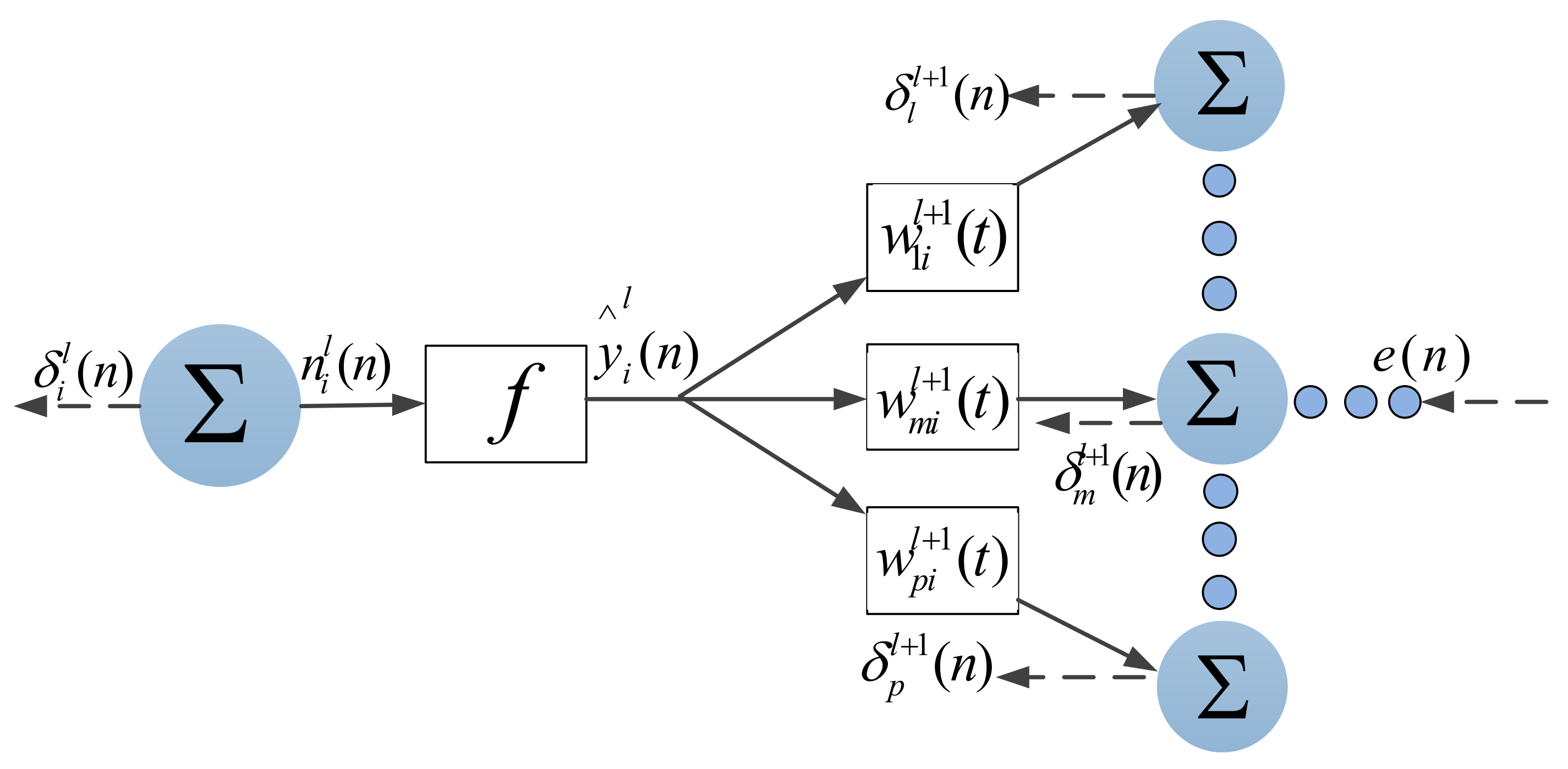
In (12), the output $\hat{y}{(n)}_{}^{(l-1)}$ is estimated through spreading on the kth train model of $x_i(n)$th input of MLP weights is adjusted into $w_{ij}^l(t)$, and the delta error (DE) phrase ${\delta }_i^l(n)$ has to be calculated. Figure 4 illustrates how to delta error ${\delta }_i^l(n)$ is iteratively computed from ${\delta }_m^{l+1}(n)$ and the (l + 1)th layer weights. Where $\hat{y}{(n)}_i^l$ is passed through all m numbers of neurons in (l + 1)th layer of NN. Hence, the error of BP formula is defined by (13) which calculates the DE from the output layer rearward to the input layer, overtaken the hidden layers.

$${\delta }_i^l(n)=\frac{\partial E_b}{\partial u_i^l(i)}={\displaystyle \sum _{m=1}^M\frac{\partial E_b}{\partial u_m^{l+1}(n)}}.\frac{\partial u_m^{l+1}(n)}{\partial u_i^l(n)}=f^{\prime }(u_i^l(n)).{\displaystyle \sum _{m=1}^M{\delta }_m^{l+1}(n).w_{mj}^l}$$

(13)

The delta error will be updated according to the adapted formulation as follows:

$$w_{ij}^l(t+1)=w_{ij}^l(t)+\eta .{\displaystyle \sum _{n=1}^n{\delta }_i^l(n)}{\hat{y}}_j^{l-1}(n)+\mu [w_{ij}^l(t)-w_{ij}^l(t-1)]+{\epsilon }_{ij}^l(t).$$

(14)

where $\eta$ and $\mu$ are named as the learning ratio and the momentum continuous parameter, respectively. To define the past weight changes effect in (14), the second term of the equation is the gradient of the mean square error corresponds to $w_{ij}^l(t)$. Moreover, the third term is defined as a momentum term that gives a procedure to reduce the mean-square error by adjusting the weight size adaptively. The last term in (14) is a minor random noise rate that will have a slight effect since the second or third terms have higher magnitudes. Giving noise to the NN during training will help the learning algorithm more robustness, which results in decrease generalization error, and faster learning.

2.4. Recurrent Dynamic Neural Network

The structure of the learning algorithm and weights adjustment at the input layer of MLP feedforward networks for dynamic networks have been so far discussed. The nonlinear autoregressive network with NARX is a recurrent dynamic network, with feedback connections enclosing several layers of the network. The NARX model is defined on the linear ARX model [64], which is used commonly in time-series modeling. ANN is employed in various applications such as smart grids. For example, NN based NARX is implemented in [64] to estimate the electrical load demand, wind speed, and state of battery charging (SOC). Furthermore, a technique is proposed in [65,66] to predict the PV power generation by applying the NN-NARX in smart grids. Choosing an accurate category of the NN is very essential and it is specified the type of system nature. Especially, the network type is influenced by the correlations between inputs and the outputs system nature. Accordingly, the feedforward neural networks system is applied when the relationship between input and output is static. On the other hand, when the relationships depend on the weather conditions and sea state parameters as external inputs. For this reason, we have proposed the recurring neural network as a proper superior due to memory functions that are embedded in their neurons. The NN-NARX is classified as a recurrent neural network (RNN). To compare with the other conventional RNN such as time series-NN, nonlinear automatic regressive (NAR) prove proposes that NN-NARX has characteristic advantages in speed convergence, accuracy, and capability of the deep learning algorithm [67]. Moreover, it should be mentioned that the other types of RNN might be also executing well, but due to environmental disturbances, such as sea conditions as external disturbances, which can affect inaccuracy of the load demand prediction in real-time or online conditions. As a result, it is also important to consider these disturbances as external inputs during neurons weight adjusting as we have noted in Section 3. Moreover, we should mention, the comparative performance of the three different kinds of RNN methods in the paper is investigated. To illustrate that this type of RNN is precise for solving the PMS challenges in DP vessels, we are used the NN-NARX model. For achieving this purpose, we have trained the NN with the offline procedure. Hence, the speed of convergence is not a significant problem in this method but, the convergence speed with minor step size plays a key role to have a successful training process in the NARX application.

For many applications, recurrent or operational training processes are not executed, and they are applying offline. Nevertheless, a precise trained NN is anticipated. In the next sections, the deviation error concerning the evaluated and predicted values by the NN-NARX performs initially in the DP controller, then through the communications appears in the PMS system for dispatching economically. Therefore, due to the precision of trained NN, accurate operation of the expert NN, the sea state historical relationship between inputs and the output of the NN-NARX is executed in this work to predict DP power demand in the various weather condition. The results show that the proposed NN-NARX based on LM-BP has a precise operation to approximate the trusting force command as a sensitive load related to weather situations. Therefore, it persuades the concept of employing the NN-NARX in this paper. The initial mathematical correlation of the proposed method in the nonlinear time- amplitude scheme is defined as:

$$y(n,t)=f(x(n,t-1),\dots ,x(n,t-T{d}_x),y(n,t-1),\dots ,y(n,t-T{d}_n))$$

(15)

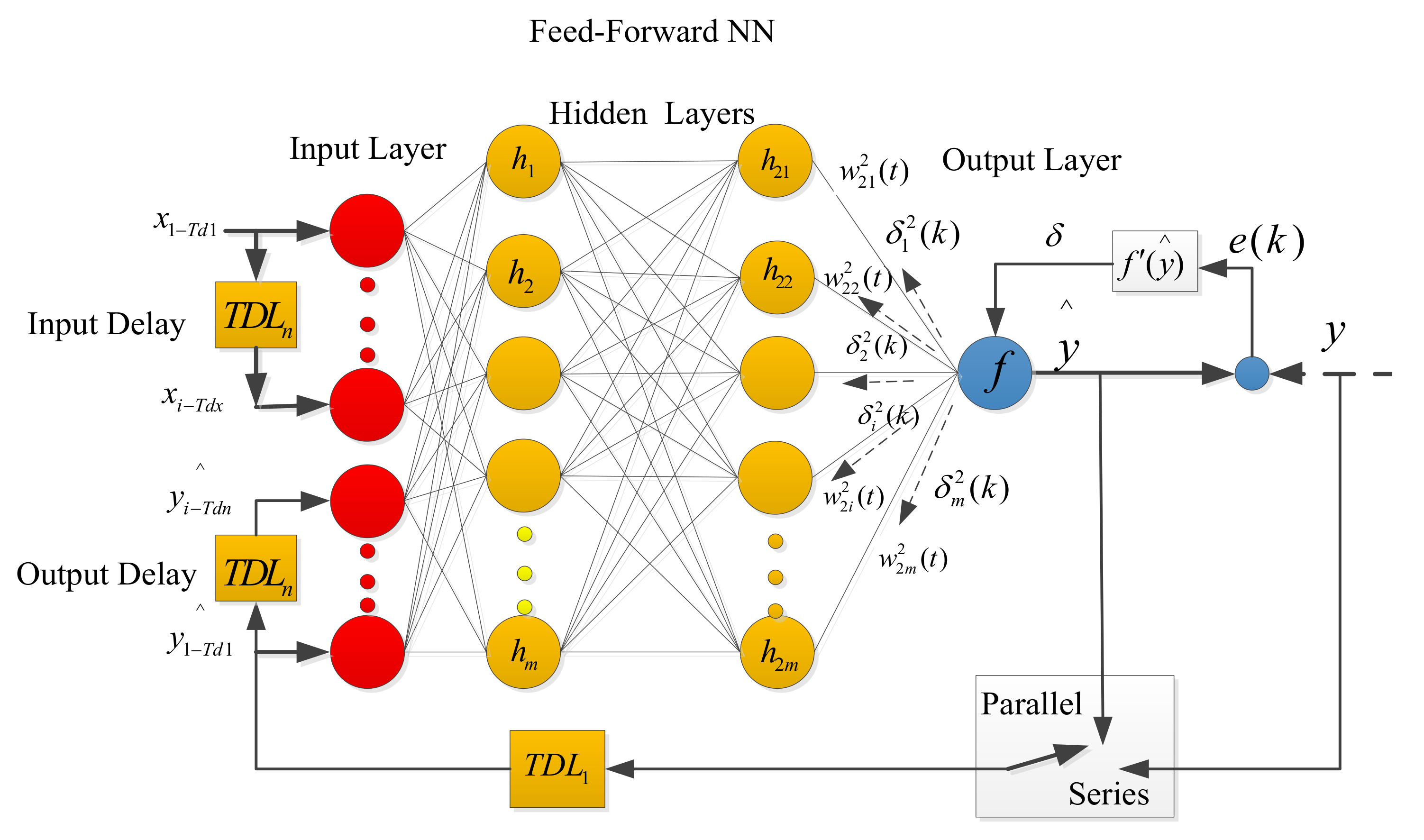
where $y(n,t)$, $x(n,t)$ and $F(x$) represent kth output sample, kth input term, and nonlinear activation function, respectively. Furthermore, $T{d}_x$ and $T{d}_y$ are integer numbers of the inputs and outputs of the NN memorial order, where they are made known the tapped delay lines (TDLs) in the RNN, respectively. Hence, the equation value of the output $y(n,t)$ in (15) is preceded by the previous values of the time delay tapped outputs and inputs. To estimate the output of the feedforward NN- NARX model, a nonlinear activation function f(x) is applied. As a result, for the training process of DP load, the preceding values of the NARX output, and input, a feed-forward series-parallel architecture is used as shown in Figure 5. Consequently, the desired output signal $\hat{y}(n,t)$ is defined in (16) based on previous values of the output signal and external input signal such as sea state as environment disturbances. Furthermore, the mathematical model of output of NARX is computed as:

$$\hat{y}(n,t)=f_{out}^{^}(\widehat{W_{out}}(f_{hid}(W_{hid}(x(n,t-1),\dots ,x(n,t-T{d}_x),y(n,t-1),\dots ,y(n,t-T{d}_n))+b_{hid}))+b_{out})$$

(16)

where $\hat{y}(n,t)$, $b_{out}$, $b_{hid}$, $\widehat{W_{out}}$ and $f_{out}^{^}$ are the predicted value of the outputs, bias vectors, hidden bias, output matrix of weights, and activation functions of the output layers, respectively. Additionally, $W_{hid}$ and $f_{hid}$ are the matrix of weights and activation functions of the hidden layers, correspondingly.

Typically, the NN feedforward learning algorithm based on LM-BP is formulated as [68]:

$$y_n(w_{ij}+d{w}_{ij})=y_n(w_{ij})+\nabla y_n{(w_{ij})}^{T}d{w}_{ij}+\frac{1}{2}\ast d{w}_{ij}{}^T{\nabla }^2{y}_n(w_{ij})d{w}_{ij}$$

(17)

In (17), $\nabla y_n{(w_{ij})}^T$ and ${\nabla }^2{y}_n(w_{ij})$ are the vector of gradient and the error function of the hessian matrix, hence the $d{w}_{ij}$ is defined as:

$$d{w}_{ij}=-{[{\nabla }^2{y}_n(w_{ij})]}^{-1}\nabla y_n(w_{ij})$$

(18)

where ${\nabla }^2{y}_n(w_{ij})=J^{T}J+S$. The $J$ is specified as the Jacobian matrix, which includes the initial network derived signal error, which is related to adjust the weights of the neuron. By considering the directional propagation algorithm, (17) is computed in (17), where $S$ expresses the second-order derivative function ${\nabla }^2{y}_n(w_{ij})$. By ignoring the $S$ in (17), the equation is solved by the Gauss–Newton method. We can also obtain results for the hessian matrix by the following approximation in (19).

$${\nabla }^2{y}_n(w_{ij})=J^{T}J+\mu I$$

(19)

To define the size of the $\mu$ coefficient of $I$ in (19) as the unit specify matrix, a scalar quantity is applied. Hence, The LM-BP algorithm is used to solve the BP scaling problem, which frequently tends to minimize the converge of the local error in preference to the global error. Moreover, BP has appropriate performance on the simple training problem; on the other hand, the BP performance will be decreased, by increasing the data and data-sizing complexity, therefore BP cannot perform discontinuously. For DP load predicting, we have faced in the environmental disturbance similar problem.

3. The Proposed Method

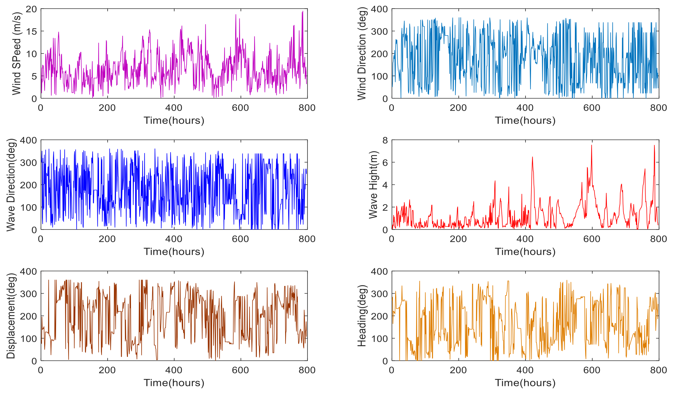
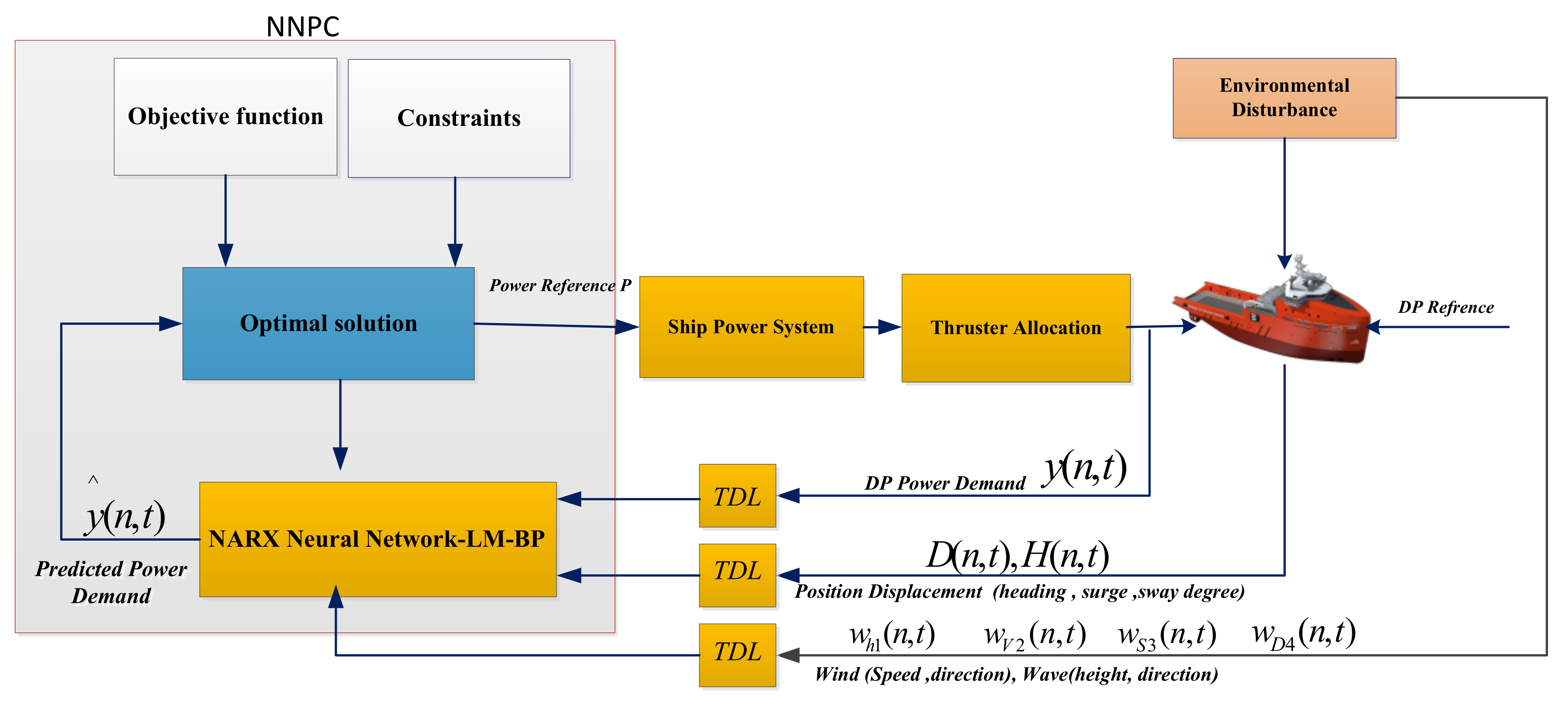
As we mentioned in Section 2, to justify the NARX equations as the proposed method and its computational procedure in (15), the following dynamic load values are used for one-day ahead prediction, where y(n,t) = {y(n,t)$\in$ t = 1, 2, …, 24} as the present DP load demand at day n, time t, $\hat{y}(n,t)$ = {$\hat{y}(n,t)$$\in$ t = 1, 2, …, 24} as the predicted DP load demand at day n, time t by the NARX network, w(n,t); is the weight vector at day n, time t and the F(U) is the nonlinear vector function representing ANN. Furthermore, the

Table 1. Parameters used in NARX-NN.

Parameter	Description		Range
$D{P}_L$	DP power (MW)	$y(n,t)$	0–7
$W_{h1}(n,t)$	wave height (m)	$x_1(n,t)$	0–8
$W_{V2}(n,t)$	wave deg (Ө)	$x_2(n,t)$	0–360
$W_{S3}(n,t)$	wind Speed (m/s)	$x_3(n,t)$	0–20
$W_{D4}(n,t)$	wind deg (Ө)	$x_4(n,t)$	0–360
$D(n,t)$	Displacement deg (Ө)	$x_5(n,t)$	0–360
$H(n,t)$	heading deg (Ө)	$x_6(n,t)$	0–360

shows the environmental disturbances according to Figure 6 where the $W_{h1}(n,t)$, $W_{V2}(n,t)$, $W_{S3}(n,t)$, $W_{D4}(n,t)$, $D(n,t)$, $H(n,t)$ are determined as wave height (m), wave swing (deg), wind speed(m/s), wind swing (deg), head swing (deg), and ship displacement (deg) as external inputs in x(n,t) = {x(n,t) $\in$ t = 1, 2, …, 24} in (15) and (16) respectively. Also tapped delay lines (TDL) values Tdy and Tdx for the NARX inputs which we have used for training the weights in (13)–(17) as shown in Figure 7 with daily DP load forecasting as 24, 48, 72, hourly from 1 to 24, and weekly 168 have been selected, respectively.

To train, validate, and test the proposed RNN method for DP load forecasting, we used real-time data from the noon report of IFDC [69]. The data noon has collected from the actual DP load profile for January 2020. The dataset also includes weather information of the sea state of the Caspian Sea, such as wave height, wind speed, wave, and wind directions, which are shown in Figure 6 and Table 1. The sea state parameters affect the thrusting power demand as a dynamic load profile, which changes with the vessel motion. To define the DP load-forecasting problem and optimal dispatching between generators in various sea conditions, we used an hourly sea state and DP load data to train the proposed NN model. The hourly data is the average of the ‘thirty’ 2 min dataset, which we collected each 2-min data set during the DP operation.

For that reason, a precise range of input parameters increases the DP demand forecasting in sea state more accuracy. Furthermore, we used the correspondence study on the historical data of thrust power consumption that determines the nonlinear and dynamic dataset of historical data, contains hourly, daily, and weekly in the DP load predicting model. The DP load demand dataset is analyzed and the load profiles are classified according to weather conditions in

Table 2. Weather parameters data patterns based on the code of sea states (data from [36]).

	Weather Conditions		Actual Power (MW)
Description	Wind (m/s)	Wave (m)
Calm-Slight	[0–5]	[0–1.25]	[0–1]
Moderate	[5–10]	[1.5–3]	[1–3]
Rough	[10–15]	[3.25–5.5]	[3–5]
High	[15–20]	[5.5–9.5]	[5–7]

. The past DP load demands and the profiles, which are the current DP load, the weather condition, and ship displacement are included affect the current load. For instance, environmental disturbances such as wave, wind, and their patterns affect the DP load demand, which leads to vessel movements. Hence, the following dynamic propulsion model is forecasted essential load demand for one hour, one day, and one week for PMS according to the Caspian Sea state, where the data has collected in a DP ship. To make the NARX, NAR, and NN with TDL, as NN-Time Series schemes which are used in the MATLAB deep learning toolbox [70]. Furthermore, the percentage of external inputs as we revealed in Table 1 is defined as 70%, 15%, and 15% for training, validating, and testing, respectively. After the definition of the percentage, the number of hidden layers neurons are adjusted 25. Finally, according to the parameters which we have defined, the NN is trained and implemented offline to predict the desired target.

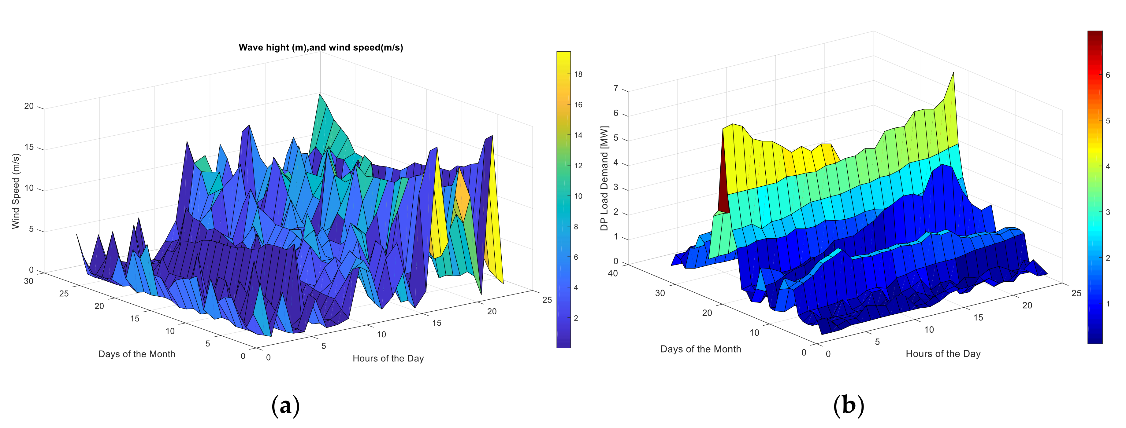
According to the collected data, as shown in Figure 6, we observed a non-linear relationship between the sea state parameters, such as wind, wave, and hourly DP load profile. Therefore, we have modeled the sea disturbances on the DP load profile as shown in Figure 8a,b. Hence, we applied hourly data of wind and wave variations and ship displacement as external inputs (disturbances) in (15) and (16) for high accuracy and speed convergence of the NARX-NN to train weights in MLP based LM-BP in (17) for DP load forecasting.

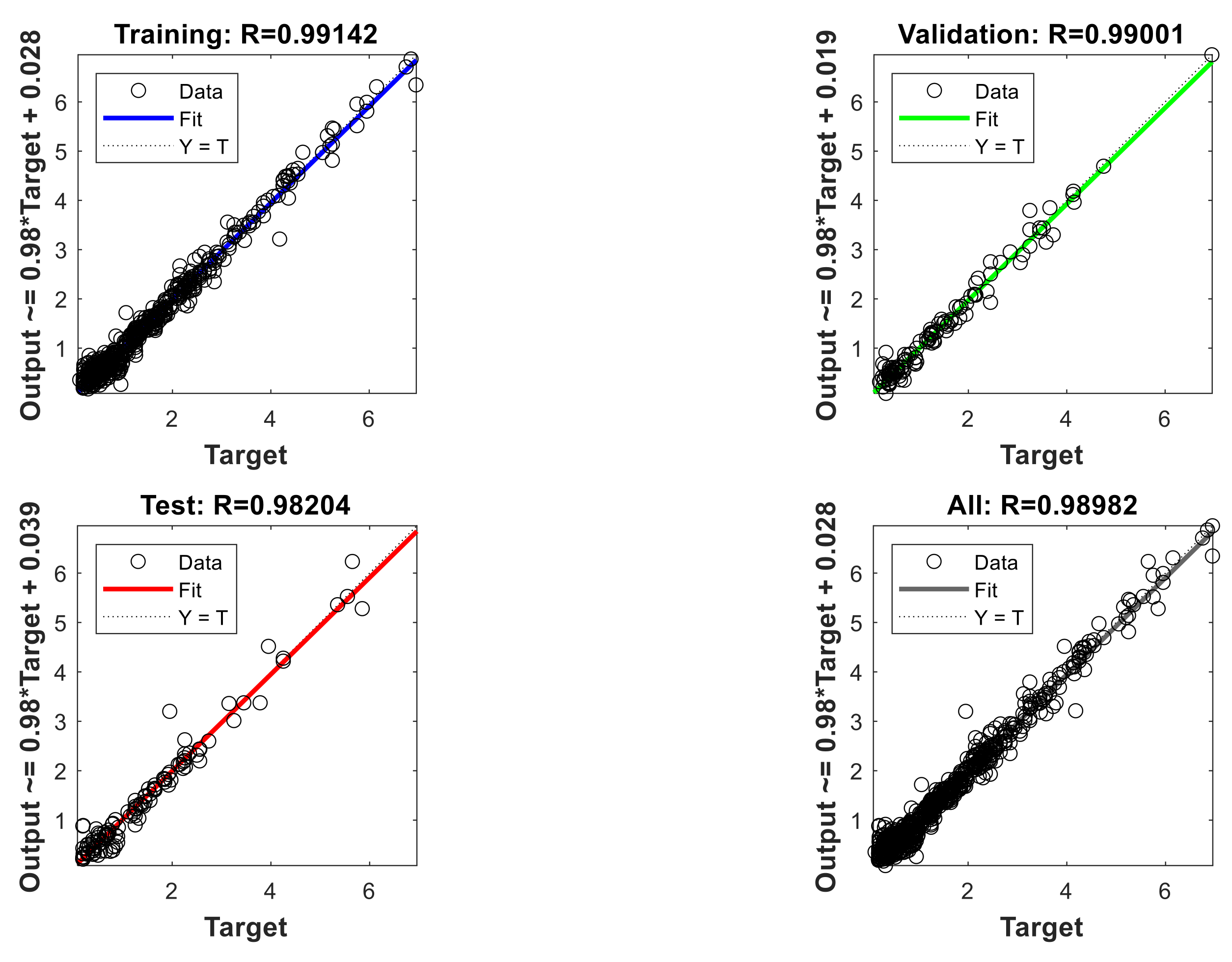
To analyze the performance of the training procedure by using the proposed method, we have validated and tested the trained data set based on actual thruster’s power consumption. Figure 9 displays the regression plots of STELF for the hourly, daily, and weekly for training, validation, and testing epochs. The regression results show that the training, validating, and testing are fairly successful where the data sets are trained more than 0.99, validated and tested values of trained parameters are around 0.99 and 0.98 at the 11 iterations. In addition, the majority of the vast data of the training collection produces result output on the edge of the first-order line, which is correlated to the best fitting connection. Accordingly, the relationship between the proposed method and target fitting line has shown that it can have a fairly good performance concerning the actual and predicted DP power demands by using the LM-BP-NARX technique. Regression figures are achieved for every single training process similarly.

In our case study, we evaluate LM-NARX, and the others time series NN based on following two performance measurement indicators are defined as follow: (a) mean absolute percentage error (MAPE), and (b) error variance ($\delta$), given as:

$$\delta =\sqrt{\frac{1}{N}{\displaystyle \sum _{i=1}^N[y(n,t)}-\hat{y}(n,t){]}^2}$$

(20)

$$MAPE=\frac{1}{N}{\displaystyle \sum _{i=1}^N\frac{\left|y(n,t)-\hat{y}(n,t)\right|}{y(n,t)}}\times 100$$

(21)

4. Test Results and Discussions

This paper considers three scenarios to evaluate the performance of the proposed method. Scenario 1 is the operation in sea conditions where the DP load in different sea states is evaluated to ensure that the proposed strategy has higher performance compared with other time series-NN schemes. Scenario 2 is a weekly load forecast in various sea conditions where the performance of DP load in the weekly thrusting profile is analyzed, which indicates the prediction of DP profile changes for days of the weeks. Finally, in Scenario 3, hourly load forecasting is proposed to estimate the peaks of DP load for thrusting the vessel at the multiples of 24-h lags at rough to high sea conditions. In addition, the performance of the NN-NARX estimate in comparison with other categories of time series NN schemes. In the continuation of this section, the results of the three executed scenarios are compared with diverse types of predictors.

4.1. Scenario 1: Operation at Sea State

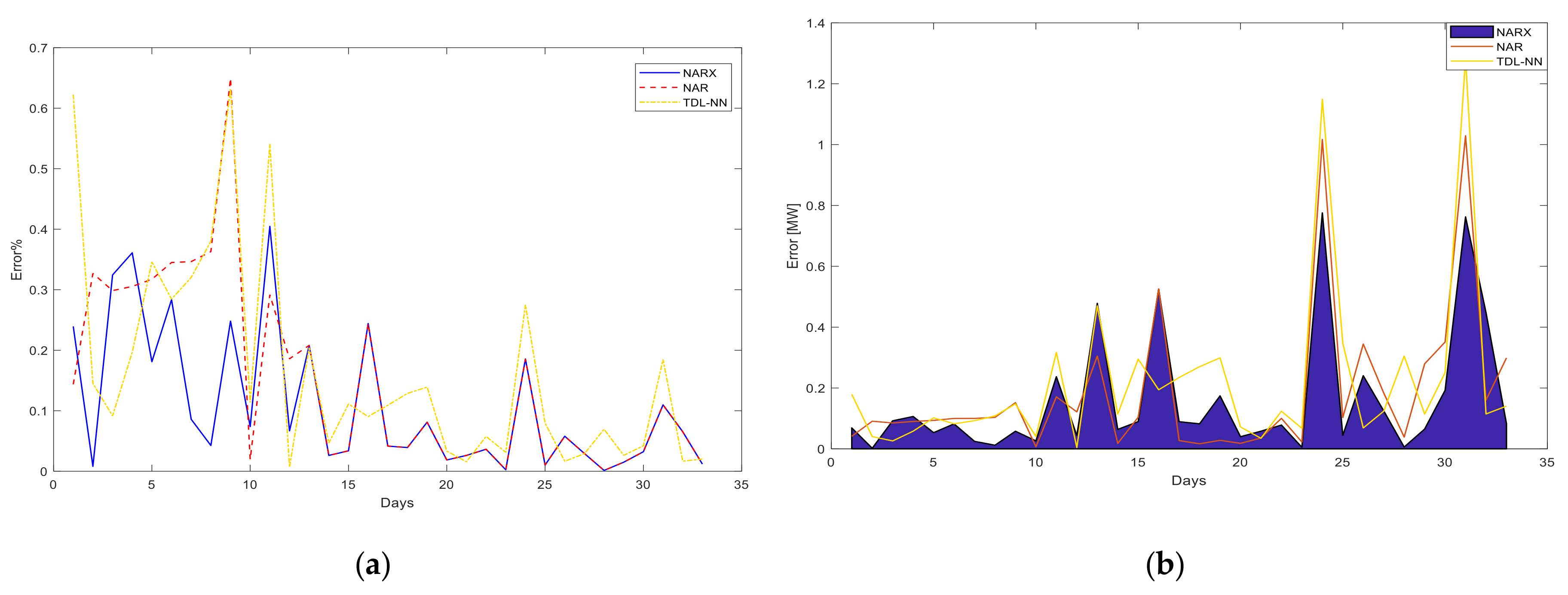
The performance of the proposed strategy to estimate average DP load patterns for the various sea condition for a month as shown in Figure 8a,b, the hourly thrusting load patterns during environmental disturbance from calm to high, such as peak load periods January 2020. We are observed that the deviations in the DP load demands for different days of the months. As shown in Figure 8b, the entire peaks load in the graph occurs in the rough to high sea conditions. Typically, the DP load demand is comparatively less on the calm-slight situation than the moderate weather condition. On calm situation days, DP load is lower than the other moderate, and rough conditions days. The results have obtained for four representative sea conditions. The weather conditions have classified as inputs, and output of the NARX model with the 168, 336, and 504 lead times as determined in Table 1 and Figure 6 for 31 days SOTLF based on sea conditions. The backpropagation learning constant and the momentum ratio in (14) have set to 0.75 and 0.1 as an initial guess, respectively. In Scenario 1, the regulating tolerance for the weights vector is selected as 0.005. The results are presented in Figure 10a,b and

Table 3. Comparison of one-month DP load forecasting in different weather conditions.

Weather Conditions	NARX		NAR		TDL-NN
	$\mathit{\delta }$ (MW)	MAPE (%)	$\mathit{\delta }$ (MW)	MAPE (%)	$\mathit{\delta }$ (MW)	MAPE (%)
Calm	0.0673	0.1933	0.0963	0.2994	0.0999	0.3067
Moderate	0.1001	0.0632	0.1071	0.0702	0.1813	0.0806
Rough	0.2095	0.0499	0.3277	0.0699	0.3514	0.0827
High	0.1238	0.0183	0.1492	0.0210	0.1533	0.0223
Average	0.1252	0.0812	0.1701	0.1151	0.1965	0.1231

in terms of the performance measurement indicators (PMIs) defined in (20) and (21). Accordingly, the average values of the MAPE and $\delta$ for LM-NARX-NN are about 0.08% and 0.13 MW, respectively. In the meantime, the maximum DP load demand error and percentage values belong to TDL-NN, which are 0.2 MW and 0.13%, respectively. In contrast, the NAR has a more accurate performance as shown in Table 3 with the $\delta$ of 0.17 MW and MAPE of 0.12% than those for the TDL-NN. However, as mentioned in Section 3, due to lack of external inputs the weather distortion cannot be considered during the offline network training.

4.2. Scenario 2: Weekly Load Forecast in Various Sea Conditions

As we have defined in Section 3, the proposed method is trained by applying the dataset for the previous seven existing days for the DP load profile. For instance, to predict the weekly load pattern, the delayed 7 × 24-h DP load profile is used as an output, and the next three latest days for thrusting demand, and environmental distortion of 72 h for inputs data, therefore we applied the numbers of TDL 24, 48 and 72 in (15) and (16), respectively. When the NN training has executed, then the NARX model progresses with one day ahead to forecast the upcoming of the 24-h DP load by employing the previous 72-h sea state data and parameters as given in Table 1 and Table 2.

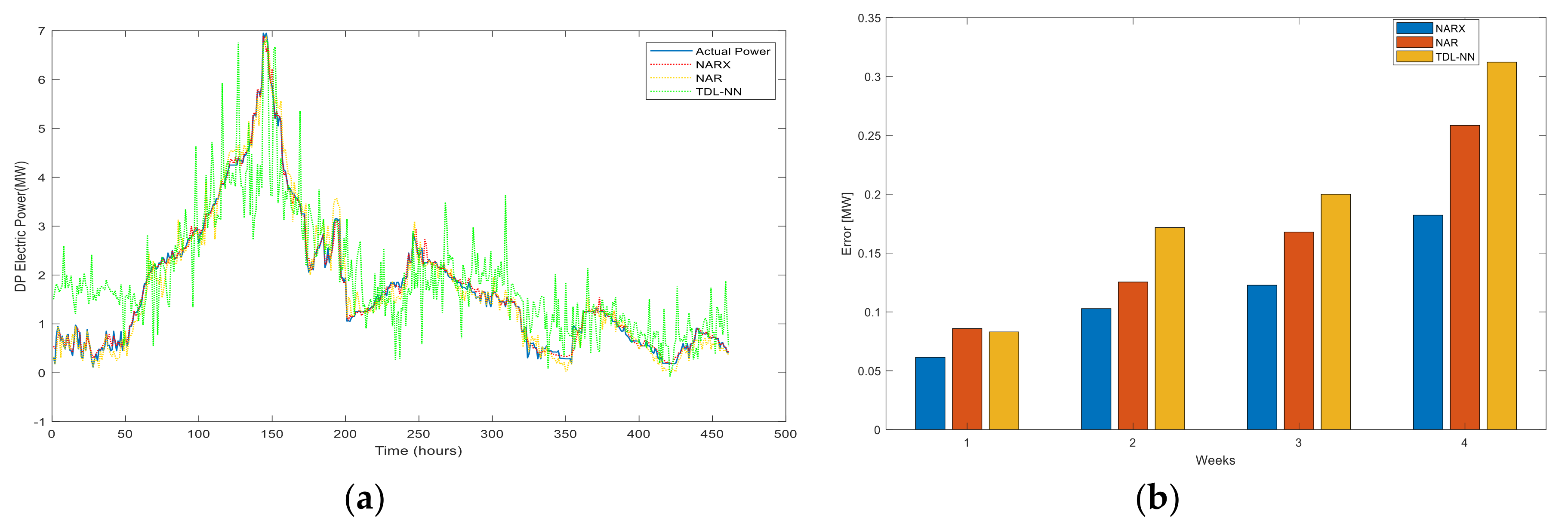
The total number of the input and hidden layers of neurons are adjusted as 7 and 25, respectively. To improve the weights vector fluctuations, one hidden layer is used with 25 different numbers of neurons and the weight vector convergence in a predefined tolerance. In this case,

Table 4. Comparison of one-month DP load forecasting in different weather conditions.

Weeks	NARX		NAR		TDL-NN
	$\mathit{\delta }$ (MW)	MAPE (%)	$\mathit{\delta }$ (MW)	MAPE (%)	$\mathit{\delta }$ (MW)	MAPE (%)
1	0.0615	0.2119	0.0859	0.2976	0.0830	0.2867
2	0.1028	0.1529	0.1254	0.2491	0.1717	0.2749
3	0.1227	0.0692	0.1679	0.0798	0.2000	0.0897
4	0.1822	0.0462	0.2585	0.0664	0.3122	0.0798
Average	0.1173	0.1200	0.1594	0.1732	0.1917	0.1827

has analyzed the average weekly DP load demand, which shows the changes in DP load profile through several days of the week. We have observed that the DP load profile has strong relation through weekdays, such as peak load periods in high sea state as shown in Figure 11a. In some of the weekdays, the thrusting demand is lower than the other weekdays due to the Calm-Slight sea state. The error percentage of DP load in MW presents in Figure 11b. The accuracy of the NARX and the minimum error percentage in Table 4 with other time-series forecasting techniques have used in the same previous network setting and evaluated. The results indicate the comparison of MAPE, error variance data of LM-NARX-BP with other time-series-NN model schemes. The minimum MAPE and $\delta$ have found nearly 0.12% and 0.12 MW, respectively by LM-NARX-NN. The maximum $\delta$, and error percentage values correspond to TDL-NN, which are about 0.2 MW and 0.18%, respectively. One the other hand, the average values of PMIs in Table 4 show that for the NAR-NN it has a more accurate performance during the weekly prediction of DP demand in sea disturbances in a month rather than TDL-NN with $\delta$ of 0.16 MW and MAPE of 0.17%, respectively. Furthermore, the NAR-NN can predict the value of DP demand to approach approximately to that obtained from the NARX-NN. Nevertheless, as mentioned in Section 3, due to uncertainties of the sea and weather conditions it would be necessary to consider disturbances as external inputs to the NARX-NN for learning procedure to recognize the sudden changes in order to obtain better results.

4.3. Scenario 3: Hourly Load Forecasting

Another significant characteristic of the DP load profile has shown in Figure 10a which provides the autocorrelation function of the hourly DP demand over four weeks. The peaks of DP profile indicate for thrusting demand at the multiples of 24-h delays at rough to high sea conditions, which shows that the load demand at the identical hours has a high relationship with each other dependent on the sea state and hours of the days as shown in Figure 8a,b. The DP load demand is categorized into hours-day and sea state patterns. The weight vector has approximated at each time intervals by applying the previous DP demand dataset for each pattern as in (15) and (16). When the weights matrix at day n, time t has been determined in (14) and (17), the thrusting force command is predicted with the DP profile data set of previous days as well as the estimated DP demand data by the network for the same day at previous time steps in (16). Hence, the adjustment of the weights vector tolerance is decreased to 0.0006 and the dataset lengths Tdx and Tdy are defined to two. Therefore, the sea state and vessel movement parameters (total 7 inputs) into the NARX model at times t, t − 1, and t − 2 of the past two days to predicted DP demand for time t + 1 of the same day. The NN with 25 hidden layers with seven neurons is used in this case.

The results have analyzed in

Table A2. Comparison of 24 h load forecasting.

Hours	NARX		NAR		TDL-NN
	$\mathit{\delta }$ (MW)	Mp (%)	$\mathit{\delta }$ (MW)	Mp (%)	$\mathit{\delta }$ (MW)	Mp (%)
1	0.0302	0.0400	0.0788	0.1196	0.2737	0.4153
2	0.1712	0.2500	0.1987	0.3015	0.0400	0.0606
3	0.3328	0.5049	0.2407	0.3652	0.3357	0.5094
4	0.3925	0.5956	0.3211	0.4872	0.0630	0.0956
5	0.1046	0.1587	0.3585	0.5440	0.0163	0.0248
6	0.1217	0.1847	0.2125	0.3225	0.2928	0.4443
7	0.0433	0.0657	0.3164	0.4802	0.4359	0.6614
8	0.1172	0.1778	0.3272	0.4965	0.0056	0.0086
9	0.0070	0.0106	0.4455	0.6761	0.5047	0.7659
10	0.6426	0.9752	0.8781	1.3324	0.5230	0.7936
11	0.2902	0.4404	0.0424	0.0644	2.0665	3.1358
12	1.8061	2.7407	0.6637	1.0071	0.2195	0.3330
13	0.4779	0.7251	0.1697	0.2575	0.6114	0.9278
14	0.2603	0.3950	0.6292	0.9547	0.1439	0.2184
15	0.0953	0.1445	0.6268	0.9511	0.4331	0.6572
16	0.2194	0.3329	0.2076	0.3150	0.2107	0.3198
17	0.1765	0.2679	0.1692	0.2567	0.1182	0.1794
18	0.0618	0.0938	0.4043	0.6136	0.5913	0.8973
19	0.2448	0.3715	0.7774	1.1797	0.0090	0.0136
20	0.0363	0.0551	0.5358	0.8131	0.1915	0.2905
21	0.0003	0.0004	0.3856	0.5851	0.4777	0.7249
22	0.1585	0.2406	0.3378	0.5126	0.8286	1.2574
23	0.1496	0.2271	1.1846	1.7976	0.9727	1.4760
24	0.3385	0.5136	0.2744	0.4164	1.7787	2.6991
Average	0.2616	0.3963	0.4077	0.6187	0.4643	0.7046

with details on hourly based for one-day ahead forecasting and presented in Figure 12a,b by the performance measurement indicators in (20) and (21). The comparison of MAPE and $\delta$ error with the other time-series-NN model schemes indicates which the minimum MAPE and $\delta$ have found 0.36% and 0.26 MW, respectively by NARX-NN. The maximum $\delta$ and error percentage values belong to TDL-NN, which are 0.46 MW and 0.7% respectively. The average error of 1 h to 24 h ahead forecasts with other time series forecasting methods have applied to the same previous network setting and evaluated in Table A2. The proposed method illustrates significant accuracy, minimum error percentage, and reliability in thrust force estimating models compared with other conventional time-series patterns.

To ensure the performance of the proposed method, the speed of convergence in the NN-training run-time is also tested and compared with those obtained from NAR and TDL-NN methods.

Table 5. Comparison of training run-time under different scenarios using different methods.

	Training Runtime (s)	NARX	NAR	TDL-NN
Scenario No.
Scenario 1		1.069	1.556	3.154
Scenario 2		1.760	1.839	38.902
Scenario 3		5.223	6.652	208.526

shows comparisons of training run-time under different scenarios using different methods. Comparisons of Figure 10, Figure 11 and Figure 12 and Table 3, Table 4 and Table 5 have shown that in contrast to other NN time series configurations, the NARX based on NN can have a fairly good performance with relatively less computation burden than other methods under different scenarios. For instance, in Scenario 3 the running time of NARX is about 5.2 s which are less than those for the NAR and TDL-NN with their running times are about 6.65 s and 208.5 s respectively. Similar results can be seen for other methods in Scenario 1 and Scenario 2.

5. Conclusions

The DP load demand predicting is already an essential part of DP vessel controllers, which the power demand from PMS for thrusting depends on weather conditions. As a result, unknown DP load demand in the future has predicted based on sea state by NARX–NN model. In this paper, we have implemented the concept of deep learning techniques, which we employed the NARX–NN as a recurrent network for DPS for operational planning, and economically dispatching between distributed generators. Hence, accurate DP load and power prediction for fixing the vessel position in this method can help the PMS to better performance in a difficult decision-making procedure for all DP vessels. The LM-NN based NARX has evaluated on real DP load profile in a PSV for thrusting the vessel position in various sea states. The proposed method confirms significant precision and defensibility in predicting technique compared with other conventional NN-time series structures. Moreover, we have trained the NARX base on the environmental disturbances as external dataset inputs to enhance the accuracy of the DP load predicting in different sea states. Furthermore, we have modernized the DP controller to forecast load by NARX-NN as a dynamic neural network, including recruited delay lines that they used for nonlinear filtering and prediction. This innovative method provides an integrated DP controller with PMS to increase the prediction accuracy of the DP load demand with the aim of enhancing operational planning in different sea conditions. In addition, three scenarios are considered for hourly, daily, and weekly load forecasting in different sea states. By using the environment disturbances dataset as external inputs in the NARX-NN, which effects on DP load demand, the proposed method can allow the PMS to increase the accuracy of short-term load prediction and operational planning for DP vessel power plant.

References

1. Fossen, T.I. Guidance and Control of Ocean Vehicles. Ph.D. Thesis, University of Trondheim, Trondheim, Norway, 1999. [Google Scholar]
2. Fossen, T.I. A survey on nonlinear ship control: From theory to practice. IFAC Proc. Vol. 2000, 33, 1–16. [Google Scholar] [CrossRef]
3. Grimble, M.; Patton, R.; Wise, D. The design of dynamic ship positioning control systems using extended Lalman filtering techniques. In Proceedings of the OCEANS’ 79, San Diego, CA, USA, 17–19 September 1979; pp. 488–497. [Google Scholar]
4. Balchen, J.; Jenssen, N.; Mathisen, E.; Saelid, S. Dynamic positioning of floating vessels based on Kalman filtering and optimal control. In Proceedings of the 1980 19th IEEE Conference on Decision and Control including the Symposium on Adaptive Processes, Albuquerque, NM, USA, 10–12 December 1980; pp. 852–864. [Google Scholar]
5. Grimble, M.; Patton, R.; Wise, D. Use of Kalman filtering techniques in dynamic ship-positioning systems. IEE Proc. D Control. Theory Appl. 1980, 127, 93. [Google Scholar] [CrossRef]
6. Saelid, S.; Jenssen, N.; Balchen, J. Design and analysis of a dynamic positioning system based on Kalman filtering and optimal control. IEEE Trans. Automat. Contr. 1983, 28, 331–339. [Google Scholar] [CrossRef]
7. Fossen, T.I.; Pérez, T. Kalman filtering for positioning and heading control of ships and offshore rigs. IEEE Control. Syst. 2009, 29, 32–46. [Google Scholar] [CrossRef]
8. Fossen, T.I.; Grovlen, A. Nonlinear output feedback control of dynamically positioned ships using vectorial observer backstepping. IEEE Trans. Control Syst. Technol. 1998, 6, 121–128. [Google Scholar] [CrossRef]
9. Fossen, T.I.; Strand, J.P. Passive nonlinear observer design for ships using lyapunov methods: Full-scale experiments with a supply vessel. Automatica 1999, 35, 3–16. [Google Scholar] [CrossRef]
10. Loria, A.; Fossen, T.I.; Panteley, E. A separation principle for dynamic positioning of ships: Theoretical and experimental results. IEEE Trans. Control Syst. Technol. 2000, 8, 332–343. [Google Scholar] [CrossRef] [Green Version]
11. Sørensen, A.J.; Sagatun, S.I.; Fossen, T.I. Design of a dynamic positioning system using model-based control. Control Eng. Pract. 1996, 4, 359–368. [Google Scholar] [CrossRef]
12. Fossen, T.I.; Paulsen, M.J. Adaptive feedback linearization applied to steering of ships. In Proceedings of the IEEE Conference on Control Applications, Dayton, OH, USA, 13–16 September 1992; pp. 1088–1093. [Google Scholar]
13. Candeloro, M.; Sørensen, A.J.; Longhi, S.; Dukan, F. Observers for dynamic positioning of ROVs with experimental results. IFAC Proc. Vol. 2012, 45, 85–90. [Google Scholar] [CrossRef]
14. Yamamoto, F.M.; Morooka, C. Dynamic positioning system of the semi-submersible platform using fuzzy control. J. Braz. Soc. Mech. Sci. Eng. 2005, 27, 449–455. [Google Scholar] [CrossRef] [Green Version]
15. Hu, X.; Du, J.; Shi, J. Adaptive fuzzy controller design for dynamic positioning system of vessels. Appl. Ocean Res. 2015, 53, 46–53. [Google Scholar] [CrossRef]
16. Tao, W.; Shaocheng, T. Adaptive fuzzy robust control for nonlinear system with dynamic uncertainties based on backstepping. In Proceedings of the International Conference on Innovative Computing Information and Control, Liaoning, China, 18–20 June 2008. [Google Scholar]
17. Chin, C.S.; Lio, C.S. Sliding-mode control of STENA DRILLMAX drillship with environmental disturbances for dynamic positioning. In Proceedings of the 11th International Conference on Modelling, Identification and Control, Tianjin, China, 13–15 July 2019; pp. 99–111. [Google Scholar]
18. Stephens, R.J.; Burnham, K.J.; Reeve, P.J. A practical approach to the design of fuzzy controllers with application to dynamic ship positioning. IFAC Proc. Vol. 1995, 28, 370–377. [Google Scholar] [CrossRef]
19. He, H.; Xu, S.; Wang, L. Mitigating surge–pitch coupled motion by a novel adaptive fuzzy damping controller for a semisubmersible platform. J. Mar. Sci. Technol. 2020, 25, 234–248. [Google Scholar] [CrossRef]
20. Wang, Y.; Zhang, X.; Fu, Y.; Ding, F.; Fu, M.; Wang, C. Adaptive fuzzy sliding mode controller for dynamic positioning of FPSO vessels. In Proceedings of the OCEANS, Marseille, France, 17–20 June 2019. [Google Scholar]
21. Fang, M.C.; Lee, Z.Y. Application of neuro-fuzzy algorithm to a portable dynamic positioning control system for ships. Int. J. Nav. Archit. Ocean Eng. 2016, 8, 38–52. [Google Scholar] [CrossRef] [Green Version]
22. Du, J.; Yang, Y.; Wang, D.; Guo, C. A robust adaptive neural networks controller for maritime dynamic positioning system. Neurocomputing 2013, 110, 128–136. [Google Scholar] [CrossRef]
23. Jang, J.S.R.; Sun, C. Neuro-fuzzy modeling and control. Proc. IEEE 1995, 83, 378–406. [Google Scholar] [CrossRef]
24. Sørensen, A.J. A survey of dynamic positioning control systems. Annu. Rev. Control 2011, 35, 123–136. [Google Scholar] [CrossRef]
25. Nguyen, T.D.; Sørensen, A.J.; Quek, S.T. Design of hybrid controller for dynamic positioning from calm to extreme sea conditions. Automatica 2007, 43, 768–785. [Google Scholar] [CrossRef]
26. Fossen, T.I. Handbook of Marine Craft Hydrodynamics and Motion Control. IEEE Control Syst. 2016, 36, 78–79. [Google Scholar]
27. Ambrosovskaya, M.E. Design and control session approach for advanced testing of DP control system. In Proceedings of the MTS DP Conference, Houston, TX, USA, 14–15 October 2014. [Google Scholar]
28. Donnarumma, S.; Figari, M.; Martelli, M.; Vignolo, S.; Viviani, M. Design and validation of dynamic positioning for marine systems: A case study. IEEE J. Ocean. Eng. 2018, 43, 677–688. [Google Scholar] [CrossRef] [Green Version]
29. Dynamic Positioning System, Dual Redundant-K-Pos DP-21/22-Kongsberg Maritime. Available online: https://www.km.kongsberg.com/ks/web/nokbg0240.nsf/AllWeb/A18DA50D246AC221C1256A46002D6505?OpenDocument. (accessed on 25 December 2018).
30. Sotnikova, M.V.; Veremey, E.I. Dynamic positioning based on nonlinear MPC. IFAC Proc. Vol. 2013, 46, 37–42. [Google Scholar] [CrossRef]
31. Veksler, A.; Johansen, T.A.; Borrelli, F.; Realfsen, B. Dynamic positioning with model predictive control. IEEE Trans. Control Syst. Technol. 2016, 24, 1340–1353. [Google Scholar] [CrossRef] [Green Version]
32. Zhang, H.; Rudy, N.R.; Lodewijks, G. Trajectory tracking of autonomous vessels using model predictive control. IFAC Proc. Vol. 2014, 47, 8812–8818. [Google Scholar] [CrossRef] [Green Version]
33. Yan, Z.; Wang, J. Model predictive control for tracking of underactuated vessels based on recurrent neural networks. IEEE J. Ocean. Eng. 2012, 37, 717–726. [Google Scholar] [CrossRef]
34. Chen, H.; Wan, L.; Wang, F.; Zhang, G. Model predictive controller design for the dynamic positioning system of a semi-submersible platform. J. Mar. Sci. Appl. 2012, 11, 361–367. [Google Scholar] [CrossRef]
35. Zheng, H.; Wu, J.; Wu, W.; Zhang, Y. Robust dynamic positioning of autonomous surface vessels with tube-based model predictive control. Ocean. Eng. 2020, 199, 106820. [Google Scholar] [CrossRef]
36. Cheng, X.; Li, G.; Ellefsen, A.L.; Chen, S.; Hildre, H.P.; Zhang, H. A Novel Densely Connected Convolutional Neural Network for Sea State Estimation Using Ship Motion Data. IEEE Trans. Instrum. Meas. 2020, 1. [Google Scholar] [CrossRef]
37. Zhao, F.; Yang, W.; Tan, W.W.; Yu, W.; Yang, J.; Chou, S.K. Power management of vessel propulsion system for thrust efficiency and emissions mitigation. Appl. Energy 2016, 161, 124–132. [Google Scholar] [CrossRef]
38. Veksler, A.; Johansen, T.A.; Skjetne, R. Thrust allocation with power management functionality on dynamically positioned vessels. In Proceedings of the American Control Conference, Montreal, QC, Canada, 27–29 June 2012; pp. 1468–1475. [Google Scholar]
39. Shen, Q.; Ramachandran, B.; Srivastava, S.K.; Andrus, M.; Cartes, D.A. Power and energy management in integrated power system. In Proceedings of the 2011 IEEE Electric Ship Technologies Symposium, Alexandria, VA, USA, 10–13 April 2011; pp. 414–419. [Google Scholar]
40. Veksler, A.; Johansen, T.A.; Skjetne, R.; Mathiesen, E. Thrust allocation with dynamic power consumption modulation for diesel-electric ships. IEEE Trans. Control Syst. Technol. 2016, 24, 578–593. [Google Scholar] [CrossRef] [Green Version]
41. Mehrzadi, M.; Su, C.-L.; Terriche, Y.; Vasquez, J.C.; Guerrero, J.M. Operation Planning of Standalone Maritime Power Systems Using Particle Swarm Optimization. In Proceedings of the 2019 1st International Conference on Electrical, Control and Instrumentation Engineering (ICECIE), Kuala Lumpur, Malaysia, 25 November 2019; pp. 1–6. [Google Scholar]
42. Anvari-Moghaddam, A.; Dragicevic, T.; Meng, L.; Sun, B.; Guerrero, J.M. Optimal planning and operation management of a ship electrical power system with energy storage system. In Proceedings of the 42nd Annual Conference of the IEEE Industrial Electronics Society, Florence, Italy, 23–26 October 2016; pp. 2095–2099. [Google Scholar]
43. Skjong, E.; Johansen, T.A.; Molinas, M.; Sorensen, A.J. Approaches to Economic Energy Management in Diesel-Electric Marine Vessels. IEEE Trans. Transp. Electrif. 2017, 3, 22–35. [Google Scholar] [CrossRef] [Green Version]
44. Ganguly, A.; Goswami, K.; Mukherjee, A.; Sil, A.K. Short-term load forecasting for peak load reduction using artificial neural network technique. In Advances in Computer, Communication and Control. Lecture Notes in Networks and Systems Proceedings of the Advances in Computer, Communication and Control; Biswas, U., Banerjee, A., Pal, S., Biswas, A., Sarkar, D., Haldar, S., Eds.; Springer: Singapore, February 2019; Volume 41, pp. 551–559. [Google Scholar]
45. Azad, H.B.; Mekhilef, S.; Gounder, V. Long-term wind speed forecasting and general pattern recognition using neural network. IEEE Trans. Sustain. Energy 2014, 5, 546–553. [Google Scholar] [CrossRef]
46. Taylor, J.W. Short-term electricity demand forecasting using double seasonal exponential smoothing. J. Oper. Res. Soc. 2003, 54, 799–807. [Google Scholar] [CrossRef]
47. Quan, H.; Srinivasan, D.; Khosravi, A. Short-term load and wind power forecasting using neural network-based prediction intervals. IEEE Trans. Neural Netw. Learn. Syst. 2014, 25, 303–315. [Google Scholar] [CrossRef]
48. Li, D.; Jayaweera, S.K. Uncertainty modeling and prediction for customer load demand in smart grid. In Proceedings of the 2013 IEEE Energytech, Cleveland, OH, USA, 21–23 May 2013; pp. 1–6. [Google Scholar]
49. Cheng, L.; Bao, Y. Short-term power load forecasting based on empirical mode decomposition and deep neural network. In Proceedings of the Purple Mountain Forum International Forum on Smart Grid Protection and Control, Nanjing, China, 17–18 August 2019; pp. 757–768. [Google Scholar]
50. Singhal, R.; Choudhary, N.K.; Singh, N. Short-Term Load Forecasting Using Hybrid ARIMA and Artificial Neural Network Model. Lect. Notes Electr. Eng. 2019, 935–947. [Google Scholar] [CrossRef]
51. Ahmed, K.M.U.; Ampatzis, M.; Nguyen, P.H.; Kling, W.L. Application of time series and artificial neural network models in short term load forecasting for scheduling of storage devices. In Proceedings of the 49th International Universities Power Engineering Conference (UPEC), Cluj-Napoca, Romania, 2–5 September 2014. [Google Scholar]
52. Garulli, A.; Paoletti, S.; Vicino, A. Models and techniques for electric load forecasting in the presence of demand response. IEEE Trans. Control Syst. Technol. 2015, 23, 1087–1097. [Google Scholar] [CrossRef]
53. Ebberley, A.W.; Gao, D.W. Study of artificial neural network-based short term load forecasting. In Proceedings of the 2013 IEEE Power & Energy Society General Meeting, Vancouver, BC, Canada, 21–25 July 2013; pp. 1–4. [Google Scholar]
54. Ricalde, L.J.; Cruz, B.; Catzin, G.; Alanis, A.Y.; Sanchez, E.N. Forecasting for smart grid applications with higher-order neural networks. In Proceedings of the World Automation Congress 2012, Puerto Vallarta, Mexico, 24–28 June 2012; pp. 1–6. [Google Scholar]
55. Feilat, E.A.; Bouzguenda, M. Medium-term load forecasting using neural network approach. In Proceedings of the 2011 IEEE PES Conference on Innovative Smart Grid Technologies-Middle East, Jeddah, Saudi Arabia, 17–20 December 2011; pp. 1–5. [Google Scholar]
56. Wai, R.J.; Huang, Y.C.; Chen, Y.C. Intelligent daily load forecasting with fuzzy neural network and particle swarm optimization. In Proceedings of the 2012 IEEE International Conference on Fuzzy Systems, Brisbane, CA, USA, 10–15 June 2012; pp. 1–6. [Google Scholar]
57. Coelho, V.N.; Guimarães, F.G.; Reis, A.J.R.; Coelho, I.M.; Coelho, B.N.; Souza, M.J.F. A heuristic fuzzy algorithm bio-inspired by evolution strategies for energy forecasting problems. In Proceedings of the 2014 IEEE International Conference on Fuzzy Systems (FUZZ-IEEE), Beijing, China, 6–11 July 2014; pp. 338–345. [Google Scholar]
58. Marinescu, A.; Harris, C.; Dusparic, I.; Cahill, V.; Clarke, S. A hybrid approach to very small scale electrical demand forecasting. In Proceedings of the 2014 IEEE PES Innovative Smart Grid Technologies, Washington, DC, USA, 19–22 February 2014; pp. 1–5. [Google Scholar]
59. Sahay, K.B.; Tripathi, M.M. Day ahead hourly load forecast of PJM electricity market and ISO New England market by using artificial neural network. In Proceedings of the IEEE Innovative Smart Grid Technologies -Asia, Washington, DC, USA, 10–13 November 2013. [Google Scholar]
60. Soman, S.S.; Zareipour, H.; Malik, O.; Mandal, P. A review of wind power and wind speed forecasting methods with different time horizons. In Proceedings of the North American Power Symp. (NAPS), Arlington, TX, USA, 26–28 September 2010; pp. 1–8. [Google Scholar]
61. Mehrzadi, M.; Terriche, Y.; Su, C.-L.; Othman, M.B.; Vasquez, J.C.; Guerrero, J.M. Review of Dynamic Positioning Control in Maritime Microgrid Systems. Energies 2020, 13, 3188. [Google Scholar] [CrossRef]
62. Hunt, K.J.; Sbarbaro, D.; Zbikowski, R.; Gawthrop, P.J. Neural networks for control systems—A survey. Automatica 1992, 28, 1083–1112. [Google Scholar] [CrossRef]
63. Willis, M.J.; Montague, G.A.; di Massimo, C.; Tham, M.T.; Morris, A.J. Artificial neural networks in process estimation and control. Automatica 1992, 28, 1181–1187. [Google Scholar] [CrossRef]
64. Le, V.M.; Pham, B.T.; Le, T.T.; Ly, H.B.; Le, L.M. Daily rainfall prediction using nonlinear autoregressive neural network. In Micro-Electronics and Telecommunication Engineering Lecture Notes in Networks and Systems; Sharma, D., Balas, V., Son, L., Sharma, R., Cengiz, K., Eds.; Springer: Singapore, 2020; Volume 106. [Google Scholar]
65. Lipu, M.S.H.; Hannan, M.A.; Hussain, A.; Saad, M.H.M.; Ayob, A.; Blaabjerg, F. State of charge estimation for lithium-ion battery using recurrent narx neural network model based lighting search algorithm. IEEE Access 2018, 6, 28150–28161. [Google Scholar] [CrossRef]
66. Raza, M.Q.; Mithulananthan, N.; Li, J.; Lee, K.Y.; Gooi, H.B. An ensemble framework for day-ahead forecast of pv output power in smart grids. IEEE Trans. Ind. Inf. 2019, 15, 4624–4634. [Google Scholar] [CrossRef] [Green Version]
67. Siegelmann, H.T.; Horne, B.G.; Giles, C.L. Computational capabilities of recurrent NARX neural networks. IEEE Trans. Syst. Man Cybern. 1997, 27, 208–215. [Google Scholar] [CrossRef] [Green Version]
68. Raza, M.Q.; Baharudin, Z.; Nallagownden, P. comparative analysis of PSO and LM based NN short term load forecast with exogenous variables for smart power generation. In Proceedings of the 5th International Conference on Intelligent and Advanced Systems (ICIAS), Kuala Lumpur, Malaysia, 3–5 June 2014; pp. 1–6. [Google Scholar]
69. Iran Fajr Marine, Drilling and Engineering Services Co. Available online: http://www.iranfajr.com (accessed on 20 April 2020).
70. Neural Network Toolbox, Create Create, Train, and Simulate Shallow and Deep Learning Neural Networks. Available online: https://www.mathworks.com/products/neural-network.html (accessed on 27 July 2018).
Figure 1. (a) Schematic of a generic feed-forward network and (b) a typical MLP structure with neuron interconnections.
Applsci 10 04889 g001
Figure 2. A Single neuron for back-propagation training MLP model.
Applsci 10 04889 g002
Figure 3. A multiple-layer MLP neural network model.
Applsci 10 04889 g003
Figure 4. The EBP computing method for MLP.
Applsci 10 04889 g004
Figure 5. The typical structural design of NN-NARX series-parallel modes with error back-propagation computing method with TDL values Tdy and Tdx as network output and input memory respectively.
Applsci 10 04889 g005
Figure 6. Historical data patterns of weather parameters, and Vessel displacement for the period one month of offshore operation.
Applsci 10 04889 g006
Figure 7. Schematic diagram of NARX-NN based LM-BP that used in training procedure by considering environmental disturbances, and vessel motion.
Applsci 10 04889 g007
Figure 8. (a). Relationship model between wind speed and wave height as inputs for short terms load forecasting and (b) DP load profile for January 2020.
Applsci 10 04889 g008
Figure 9. Analysis of the LM-BP-NARX regression model.
Applsci 10 04889 g009
Figure 10. (a) The proposed model comparison for the SOTLF for 31 days ahead forecasting error percentage, and (b) error variance in MW.
Applsci 10 04889 g010
Figure 11. (a) The proposed method comparison for SOTLF for two weeks ahead forecasting error percentage, and (b) error variance in MW for weeks in a month.
Applsci 10 04889 g011
Figure 12. (a) The proposed method comparison in SOTLF for with 24 h lead times, and (b) error Percentage in MW.
Applsci 10 04889 g012