Attributes Reduction in Big Data

Abstract

Processing big data requires serious computing resources. Because of this challenge, big data processing is an issue not only for algorithms but also for computing resources. This article analyzes a large amount of data from different points of view. One perspective is the processing of reduced collections of big data with less computing resources. Therefore, the study analyzed 40 GB data to test various strategies to reduce data processing. Thus, the goal is to reduce this data, but not to compromise on the detection and model learning in machine learning. Several alternatives were analyzed, and it is found that in many cases and types of settings, data can be reduced to some extent without compromising detection efficiency. Tests of 200 attributes showed that with a performance loss of only 4%, more than 80% of the data could be ignored. The results found in the study, thus provide useful insights into large data analytics.

1. Introduction

The recent sharp increase in technological development and the associated growing increase in the volume of data spread and produced have led to regular data being converted into big data. As the name implies, big data indicates the type of data of large size, the forms it includes, and requiring high-speed servers for timely input [1]. Big data is the variability, size, and speed of data that needs to be achieved. This data is normally saved in large servers and is available only when necessary [2]. Big data is used to perform regular organizational processes, such as decision making and validation [3]. However, to improve efficiency, a trade-off is critical between efficiency and application size [4]. Typical examples are GPS, facial recognition cameras. The effectiveness of such sort of applications can be improved by providing large datasets for model training. Alternatively, this is not possible because large data sets need comparatively large storage space, which becomes difficult to manipulate. For this, a mechanism is needed that allows big data subgroups to carry knowledge and information similar to those found in the source data [5].

Big data also poses serious account risks that need to be processed to ensure end-user protection at the end. Accordingly, some parameters are usually indicated to ensure the quality of big data and the quality of information [6]. Examples of these parameters are: syntactical validity, appropriate attribute association, Precision, theoretical relevancy, controls, and audibility [6]. In addition, other problems are created by the management of servers, privileges, sorting, and security [7]. By 2002, the number of digital devices exceeded 92% with five Exabytes of data [8], which has been increasing since then leading the problem to develop gradually. Today, the business of big data is about $46.4 billion [8], which means that, despite problems with data processing, user interest is increasing over the years. Relative to data mining, data processing becomes very difficult with hundreds of groups classified by small differences, increased workload, and compilation time [8].

In addition to endless applications, big data has become a complex concept for data mining, information fusion, social networks, semantic network, etc. [9]. Accordingly, much attention was paid to data processing, pattern mining, data storage, analysis of user behavior, data visualization, and data tracking [10].

This devastation is intensified by the search for solutions to the problems of a large collection due to the fact that technologies such as machine learning, computational intelligence, and social networks use libraries to process data. These libraries, consecutively, increase in size as their scope expands. As a result, solutions are constantly being sought for ease of processing and scanning of big data. These solutions are data sampling, data condensation, density-based approaches, incremental learning, divide and conquer, distributed computing, and others [8].

From data handling perspectives, sampling big data has the most considerable concern of complexity, computational burden, and inefficiency for the appropriate execution of the task [11]. The effort of sampling is the number of data sets that can be added to each sample. In general, it is believed that the richness of these data sets is poor only if the sample is biased by estimation [12]. In this regard, the selection bias can be calculated and successfully determined using the reverse sampling procedure, where information is used from external resources, or using digital integration technology, where big data is combined with independent probabilistic sampling [13]. Sample size is very critical and plays a significant role in the accuracy of a system [14]. Thus, as a solution to the challenges of sampling big data, some algorithms have been introduced, such as the process of Zig Zag [15], nonprobabilistic sampling [13], inverse, and cluster sampling [16].

Machine learning is a data analysis that learns from the available data for prediction and decision making [16]. Trends in data are extracted and calculated for machine learning techniques. These machines are designed to understand information and are able to extract some meaning from them. Training is carried out through comparisons, communication, strategies, discoveries, problem solving, search, and comparison with changing parameters. The ability of any device to learn depends on the amount of information with which it can work, and the amount that can be processed [4]. Machine learning improves as the amount of input data increases, however, the algorithms used are usually traditional and designed to deal with simple data sets, which makes the job even harder. Some challenges in regard to big data include but not limited to memory and processing problems, unstructured data forms, rapidly changing data, and unclassified data [17].

Deep learning in the form of the Convolutional Neural Networks (CNNs) is used to accurately model classification data [18], particularly image and text data. The interest towards CNN-based recognition and detection has further increased in recent years. This is due to its improved classification and detection performance in the imaging domain. On the other hand, CNNs require a huge amount of processing power for large datasets. In its simplest form, the CNN requires several convolution layers, pooling layers, and the fully connected layers, thus requiring considerable resources and time to train and learn the distribution of the features. In large networks, for example, GNET, VGG16, time complexity, and resource requirements increase exponentially. Therefore, there is a need to analyze whether for a similar dataset, especially having strongly correlated images, should one process all the features and images of such a dataset? As such, we believe that research work in the direction of optimally reducing the dataset is of immense interest not only for traditional classical classifiers but also for deep learning models, and this thus also initiates one of the motivations for the work in this article.

Moreover, the attention has shifted from the usual to the independent feature extraction [19,20]. However, the increase of features and data instances, which have not been examined enough. The dimensionality clearly affects the performance of the final model, similarly, a steady increase in the amount of data leads to a recount and reassessment of machine learning models. This makes a huge dependence on powerful computer equipment and resources; however, these facilities are still inaccessible to the masses and many research institutes.

The work in this paper discusses the reduction of data for classification purposes and some machine learning scenarios. The study analyses the data attributes role and whether it can be generalized to big data. Attributes play a significant role in classification and model learning. At the time that more attributes are considered an advantage towards better models, they also at the same time can be complicated to a far extent if they do not cover data and classes fairly. This problem will become even worse if the data is too big which makes dimensionality a serious issue because of the large number of data attributes. For such impacts of data attributes on classifier performance, this study investigates how this impact can affect the classification performance. The experiments in the study use the video dataset available at [21], which is a massive data set consisting of more than 40 GB of video data. The data are divided into three categories for analysis purposes: Unacceptable, Flagged, and Acceptable. The study is based on the general concept of data sampling, however, it uses data from image filtering. This can be justified in the following three key points: first, the data is well organized into three categories, which represents an appropriate case for machine learning algorithms. Second, despite the data type image, it can be converted to numerical values in the feature form, which, accordingly, is equal to other data sets and similar machine learning problems. The last point is the huge size of data that exceeds 40 GB, which means the data used in the analysis is big data. As a result, the findings can be generalized to such studies with similar nature of data.

2. Related Work

Looking at the literature, there are some works such as [22,23,24,25], which propose and model such scenarios. The work in [22] combines AlexNet [20] and GoogLeNet [26] to increase productivity. The work in [24] uses color transformations. Evidence is given in [27]. In [28], the adaptive sampling method is used for filtering. Article [29] explains the analysis of the website filter, and [30] combines the analysis of key frames. [31,32] use visual functions to access multimedia and filtering. Articles [33,34,35,36] are based on content retrieval.

Another method also known as neighborhood rough sets [37] is used widely as a tool to reduce attributes in big data. Most of the existing methods cannot well describe the neighborhoods of samples. According to the authors of the [37], the proposed work is the best choice in such scenarios. The work proposed in [38] introduces a hierarchical framework for attributes reduction in big data. The authors propose a supervised classifier model. For reducing noise, Gabor filters are used that improve the overall efficiency of the proposed framework. For specific feature selection, Elephant Herd Optimization is utilized. The system architecture is implemented with a Support Vector Machine. To reduce the irrelevant attributes and keep only important attributes Raddy et al. [39] propose a method that uses two important features selection methods Linear Discriminant Analysis and Principal Component Analysis. Four machine learning algorithms Naive Bayes, Random Forest, Decision Tree Induction, and Support Vector Machine classifiers are used by the authors. In [40], the authors investigate attribute reduction in parallel through dominance-based neighborhood rough sets (DNRS). The DNSR considers the partial orders among numerical and categorical attributes. The authors present some properties of attribute reduction in DNRS, and also investigate some principles of parallel attributes reduction. Parallelization in various components of attributes is also explored in much detail. A multicriterion-based attribute-reducing method is proposed in [41], considering both neighborhood decision and neighborhood decision with some consistency. The neighborhood decision consistency calculates the variations of classification if attribute values vary. Following the new attribute reducing, a heuristic method is also proposed to derive reduct which targets to obtain comparatively less error rate. The experimental results confirm that the multicriterion-based reduction improves the decision consistencies and also brings more stable results.

3. Classification Models

In this section, we discuss the classifiers used in the experimental evaluation.

Classifiers learn the inherent structure in the data. The classification and the learning ability strongly depends on the data types, the correlation among the attributes, and the amount of clean data processed for a particular problem. We selected the SVM, Random Forest, and AdaBoost for our sampling analytics due to its good overall performance state-of-the-art for most of the correlated data problems.

Recently, tree-based classifiers have been greatly admired. This acceptance stems from the instinctive nature and the general cool training example. However, catalog trees hurt from the classification and oversimplification accuracy. It is impossible to grow equally the classification and generality accuracy concurrently and thus generalize at the same time. Leo Breiman [42] presented the Random Forest of this design. Random Forest has the advantages of a mixture of several trees from the corresponding dataset. Random Forest (RF) creates a forest of trees, so each tree is created on the basis of a random kernel of enlarged data. For the steps of classification, input is applied to each tree. Each tree decides on a vector class. The decisions are collected for final classification. The decision of the tree is called the vote of the tree in the forest. So, for example, for a specific problem, out of five trees, three trees vote “yes” and two trees vote “no”, a Random Forest classifies the problem as “yes” because a Random Forest works by a majority vote.

In the Random Forest, for growing the classification trees, let cases in the training set be N, thus sampling N data items are selected at random, but picked based on a replacement from the data set. This sample constitutes the training set for tree growth. If there are “K” variables, a small “k”, where “k” << K is specified such that, “k” number of variables being selected randomly from the large K dataset. The best split on these “k” is used to split the node, and the value of “k” is held constant during the forest growth. Each tree is allowed to grow to its largest extent possible on its part of data. There is no pruning. With the increase in tree count, the generalization error thus converges to a limit. (to be rewritten).

Support Vector Machines [43] are supervised learning methods used for classification and regression in computer vision and some other fields. Considering a study dataset consisting of two classes, SVM develops a training model. The model assigns newly sampled data to one or the other category, which makes it a nonprobabilistic binary classifier model. Data can be visualized as points in space in SVM separated by the hyperplane (gap) that is as large as possible. SVM can also be used for nonlinear classification using the kernel that maps the inputs into high-dimensional feature spaces where separation becomes easy. SVM has shown its potential in a number of classification tasks ranging from simple text classification to the imaging, audio, and deep learning domains.

Adaptive boosting (AdaBoost) [44] is yet another approach for increasing the accuracy of the classification task. The purpose of the AdaBoost method is to apply the weak classification method to repeatedly modified versions of the data [44]. This, in turn, produces a sequence of comparatively weak classifiers. The predictions are then combined through a majority vote which produces the final prediction.

4. Experimental Setup and Results

For feature extraction, we use the auto-correlogram approach. The auto-correlogram captures the spatial relationship between the color pixels.

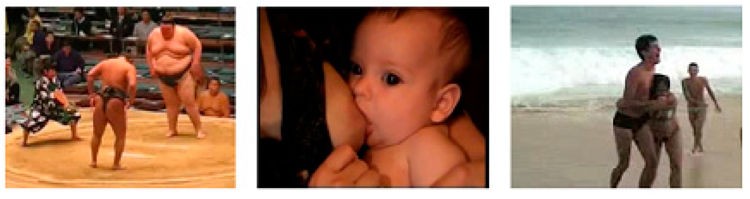
For evaluation of the architecture, we use the sampled dataset obtained from videos of NDPI, details are available in [21]. This is a large dataset which consists of around 40 GB video data. For analysis, we divide the sampled data into three classes i.e., Unacceptable, Acceptable, and Flagged. Figure 1 shows some samples.

We use the F-measure as an evaluation measure. The F-measure takes into account both the Precision and the Recall as follows:

F-measure = 2 × [(Precision × Recall)/(Precision + Recall)]

(1)

4.1. Attributes’ Role

The class attribute has a significant role in model learning. One interest of this paper is to investigate the effect of attributes in classification. Attributes have an impact on the model of data and the classification. At least theoretically, more attributes lead to a better model, however, attributes can be very complex if they do not properly cover data and classes. In other words, if attributes are not related to data categories or the relationship between attributes is not strong, increasing the number of attributes can have negative performance results. Big data usually means a lot of features. This can be a problem in two ways. Firstly, solving a large number of attributes is a problem in itself. Secondly, a large number of attributes leads to a dimensionality curse, and thus the classifier can be misleading. Thus, the classifier will not take advantage of the robust correlated attributes associated. This has serious consequences for the problem under investigation and the classifier performance. The experimental setup aims to analyze the role of attributes in data and thus generalize it to big data.

4.2. SVM

For the analysis of the attributes in the SVM classifier, we perform several experiments to analyze the role of reducing the attributes and see whether it decreases or increases performance. For this, we use the many useful approaches available in the state-of-the-art. These are:

• Subset Evaluation proposed [45]: Evaluates the importance of a reduced set of attributes taking into account the individual-based predictive capability of every attribute and measuring the redundancy between them.
• Correlation Evaluation [46]: Considers the importance of feature by analyzing the correlation between the feature and the class variable.
• Gain Ratio Evaluation [47]: Considers the importance of a feature by analyzing the gain ratio with respect to the class.
• Info Gain Evaluation [47]: Considers the importance of an attribute that measures the information gain to the corresponding class.
• OneR Evaluation [48]: Uses the OneR classifier for the attribute role in model building.
• Principal Components [49]: Evaluates transformation and the principal components analysis of the data.
• Relief Evaluation [50]: Finds the importance of an attribute by repeated sampling and considers the value of the attribute for the nearest instance of the similar and different class.
• Symmetrical Uncertain Evaluation [51]: Considers the attribute importance by measuring the symmetrical uncertainty against the class variable.

All these approaches provide a rich and complete set of feature selection methods and are representative of the complete framework for similar tasks.

Table 1. Total number of attributes selected by the different algorithms. The 200 most important features ranked according to importance are retrieved.

Approach	Attributes
Actual Attributes Before Selection	1024
Subset Evaluation	84
Correlation Evaluation	200
Gain Ratio Evaluation	200
Info Gain Evaluation	200
OneR Evaluation	200
Principal Components	258
Relief Evaluation	200
Symmetrical Uncert. Evaluation	200

shows the different approaches and the attributes selected by them. Actual features mean the attributes that are returned by feature extraction methods and not the feature selection method. The other eight starting from the Subset Evaluation are the selection methods and select the appropriate number of attributes depending on the algorithm. The Subset Evaluation selects 84 important features and discards others. The Correlation Evaluation, Gain Ration Evaluation, Info Gain Evaluation, OneR Evaluation, Relief Evaluation, and the Symmetrical Uncertain Evaluation ranks features according to the importance. The 200 most important features (returned by the importance) are selected from these algorithms. 200 attributes are enough as the Subset Evaluation selects only 84 attributes out of 1024 attributes. The Principal Components returns 258 important components from the data.

The result of the attributes selected by these algorithms are interesting, Figure 2 and Figure 3 show the corresponding feature selection algorithm and the F-measure using the classifier SVM and the Random Forest respectively. In Figure 2, SVM is used for model learning and validation. In Figure 3, the Random Forest is used for model generation and corresponding evaluation.

In Figure 2, for SVM, the F-measure of different data attributes does not have the same behavior. Although the number of selected attributes in all algorithms is less than the number of attributes of the actual data, two algorithms have higher F-measure than the F-measure of the actual data attributes. Even though the other F-measure values are less than that of actual data, the considerable reduction in the dataset by attribute selection methods should not be neglected. The F-measure of the actual data attributes which are 1024 is 0.784. The F-measure for Subset Evaluation is 0.76, Correlation Evaluation is 0.786, the Gain Ration Evaluation is 0.783, the Info Gain Evaluation is 0.77, OneR Evaluation is 0.778, Principal Components is 0.718, Relief Evaluation is 0.79, and the Symmetrical Uncertain Evaluation is 0.767. These results are interesting and shed valuable light on the attributes selection. Despite the great reduction in the actual data attributes, the Correlation Evaluation and the Relief Evaluation F-measure is slightly higher than the F-measure of the actual data attributes, which can lead to an interesting result that is the selected attributes by these two algorithms can successfully represent the actual dataset. The lowest F-measure of 0.718 is obtained for principal components. The Subset Evaluation has slightly less F-measure (0.762) than the actual attributes (0.784). From these F-measure values, it is noted that the loss in F-measure is not that large in comparison to the advantage of reducing the amount of processed dataset. Furthermore, it is quite worth mentioning that even the F-measure is increased in two cases. As the point of this article is to analyze the impact of reducing data on performance, the results show an interesting trend.

As 100% data is represented with the 1024 attributes, the attribute selection methods provide a reduced set of data. For the Subset Evaluation, 84 attributes are selected with an F-measure of 0.762. This means that while just using the 8% of data from the actual data, we get only a 2% decrease in performance. From the physical data perspectives, we can deduce that only 8 GB data, from the 100 GB will approximately give the same performance of the 100 GB data. This is even more interesting with the Correlation Evaluation and the Relief Evaluation where F-measure is slightly higher than the actual F-measure of the actual data attributes. That means the smaller set can represent the larger dataset.

4.3. Random Forest

Figure 3 shows the analysis done with the Random Forest, and has almost similar trends as Figure 2. However, in Figure 3, for the Random Forest with actual attributes of 1024, the F-measure is 0.841, and no higher F-measure has been recorded for any of the used algorithms. The F-measure for Subset Evaluation is 0.83, Correlation Evaluation is 0.824, the Gain Ration Evaluation is 0.782, the Info Gain Evaluation is 0.825, OneR Evaluation is 0.833, Principal Components is 0.806, Relief Evaluation is 0.838, and the Symmetrical Uncertain Evaluation is 0.812. Contrary to the SVM case, the Correlation Evaluation, and the Relief Evaluation F-measure is slightly lower than the actual F-measure of 0.841. The lowest F-measure of 0.782 is obtained for Gain Ration Evaluation. The Subset Evaluation has slightly less F-measure (0.83) than the actual attributes (0.841). Despite none of the F-measure values is higher than F-measure of the actual attributes, the performance can be viewed as progressing, keeping in mind the great reduction in the dataset compared to the actual data.

In general, in Figure 3, the decreasing trend in the F-measure is low compared to the number of attributes decreased. As 40 GB (100%) data is represented with the 1024 attributes, one of the beauties of the attribute selection methods is providing a reduced set of data. Instead of processing the actual set of data attributes, a reasonable performance can be achieved with a great reduction in data attributes, and consequently a great improvement in data processing and time. Let us analyze the attribute selection method. For this, we select Relief Evaluation from Figure 3. The Relief Evaluation uses 200 attributes and achieves an F-measure of 0.838. This means that while just using the 19% data from the actual data of 1024 attributes and over 40 GB, we get only a 1% decrease in classification and recognition performance. From data perspectives, only 19 GB data, from the 100 GB data will approximately give the same performance of the 100 GB data set. The OneR Evaluation has also similar results with only a 1% decrease in performance. Without a doubt, the slight decrease in performance still can be considered positively as long as a great reduction in the data processing. The lowest F-measure is Gain Ratio Evaluation, which has almost a 6% decreased performance. Even, with 6%, we get an 81% decrease in data processing and time. As the point of this article is to analyze the impact of reducing data on performance, these results show an interesting trend towards processing big data with acceptable results. One other interesting insight noted in Figure 2 and Figure 3 is that Principal Components has comparatively reduced performance. One reason is that it may not be thoroughly investigated with the other algorithms as is done in this experimentation setup. Finally, the work in this paper presents a continuation of sampling strategies of the previous work in [46,47] and thus augments the related domain with new experiments and results.

4.4. Adaptive Boosting

Figure 4 shows the analysis done using the AdaBoost approach. The AdaBoost approach is analyzed due to its inherent similarity to the Random Forest classification approach. For this analysis, the AdaBoost uses the J48 trees as the base classifier. Figure 4 shows a similar trend of the F-measure to that of the Random Forest approach. In Figure 4, for the AdaBoost, the nonreduced F-measure is 0.786, which is almost similar to that of the SVM. The F-measure for Subset Evaluation is 0.772, Correlation Evaluation is 0.772, the Gain Ration Evaluation is 0.735, the Info Gain Evaluation is 0.782, OneR Evaluation is 0.79, Principal Components is 0.758, Relief Evaluation is 0.772, and the Symmetrical Uncertain Evaluation F-measure is 0.761. From the visual perspectives, the trending of the F-measure of Figure 4 is almost similar to that of the Random Forest of Figure 3. For AdaBoost and the Random Forest, though there is a difference in actual F-measure, the trend is almost similar, which shows an interesting similarity of behavior even in large datasets, thus augmenting the overall results and analysis of the proposed work.

5. Applications of the Study

The work in this paper presents a continuation of sampling strategies of the previous work in [52,53] and thus augments the related domain with new experiments and results. The work in [52] analyzed the impact of processing the reduced amount of actual data on machine learning model performance. Subsequently, the work in [53] investigated the impact of two different random sampling techniques with two different machine learning classifiers. Complementary, the current study focused on the data attributes rather than the dataset itself. The current results supported the results of the previous studies in terms of reducing the processed data. The results discussed and presented in Figure 2 and Figure 3 showed that the performance either improved or slightly decreased. Looking at different factors in the decreasing cases, advantages like reducing processing time as well as using limited or available computing resources have been achieved in return, which makes this decrease acceptable and reasonable.

Processing large amounts of data normally require great computing resources. From this arises an issue not only on data processing but also on the availability of computing resources for most researchers. Additionally, using the actual amounts does not necessarily ensure that it is the only way to provide useful outcomes. This study provided an appropriate scenario by processing only a reduced amount of data that can lead to a reasonable performance using fewer computing resources. In this case, the processing time will be extremely reduced as well. On the other hand, the machine learning model can be achieved by processing only subsets of the actual data attributes and no need to use all the data attributes, which might be very complex if they do not properly cover data and classes.

6. Conclusions

Big data analysis requires enough computing equipment. This causes many challenges not only in data processing, but for researchers who do not have access to powerful workstations. In this paper, we analyzed a large amount of data from different points of view. One perspective is processing of reduced collections of big data with less computing resources. Therefore, the study analyzed 40 GB data to test various strategies to reduce data processing without losing the purpose of detection and learning models in machine learning. Several alternatives were analyzed, and it was found that in many cases and types of datasets, data can be reduced without compromising detection performance. Tests of 200 attributes showed that with a performance loss of only 4%, more than 80% of the data could be deleted. The experimental setup in this work is extensive, however, additional work is still required to analyze a large number of large data sets despite that this work produced valuable results. In the future, we aim to analyze several large data sets in order to obtain important analytical results.