Abstract
Minimizing time cost in time-shared operating system is the main aim of the researchers interested in CPU scheduling. CPU scheduling is the basic job within any operating system. Scheduling criteria (e.g., waiting time, turnaround time and number of context switches (NCS)) are used to compare CPU scheduling algorithms. Round robin (RR) is the most common preemptive scheduling policy used in time-shared operating systems. In this paper, a modified version of the RR algorithm is introduced to combine the advantageous of favor short process and low scheduling overhead of RR for the sake of minimizing average waiting time, turnaround time and NCS. The proposed work starts by clustering the processes into clusters where each cluster contains processes that are similar in attributes (e.g., CPU service period, weights and number of allocations to CPU). Every process in a cluster is assigned the same time slice depending on the weight of its cluster and its CPU service period. The authors performed comparative study of the proposed approach and popular scheduling algorithms on nine groups of processes vary in their attributes. The evaluation was measured in terms of waiting time, turnaround time, and NCS. The experiments showed that the proposed approach gives better results.
1. Introduction
This section is divided into two subsections; the first subsection discusses CPU scheduling, and the second subsection discusses the clustering technique.
1.1. CPU Scheduling
The mechanism for allocating and de-allocating the CPU to a process is known as CPU scheduling [1,2,3]; the portion of the operating system that carries out these functions is called the scheduler. In multi-programming systems, the number of processes in the memory is restricted by the degree of multi-programming. There are several processes in the memory waiting to receive service from the CPU, the scheduler chooses the next process to assign the CPU, waits for its processing period, and de-allocates the CPU from that process. The scheduling mechanism is the order in which processes are selected for CPU processing. The scheduling scheme may be preemptive (i.e., the CPU is assigned to a process for a certain period) or non-preemptive (i.e., once the CPU has been assigned to a process, the process keeps the CPU until it liberates the CPU either by switching to another state or by terminating). Many different CPU scheduling algorithms have been suggested. Under First Come First Served (FCFS), non-preemptive CPU-scheduling, the process that arrives first, gets executed first. Shortest Job First (SJF), non-preemptive CPU-scheduling, selects the process with the shortest burst time. The preemptive version of SJF is called Shortest Remaining Time First (SRTF); processes are placed into the ready queue as they arrive, and the existing process is removed or preempted from execution as a process with short burst time arrives, and the shorter process is executed first. Under priority scheduling, preemptive CPU-scheduling, if a new process arrived has a higher priority than the currently running process, the processing of the current process is paused and the CPU is assigned to the incoming new process [4].
RR scheduling is the most common of the preemptive scheduling algorithms [5], referred to hereafter as Standard RR (SRR), used in real-time operating systems and timesharing [6,7]. In RR scheduling, the operating system is driven by a regular interrupt. Processes are selected in a fixed sequence for execution [8]. A process receiving CPU service is interrupted by the system timer after a short fixed interval called time slice which usually is much shorter than the CPU service period (or CPU burst) of the process [9,10,11]. After that interruption, the scheduler performs a context switch to the next process selected from the ready queue which is treated as a circular queue [12,13]. Thus, all processes in the queue are given a chance to receive service for a short fixed period. This scheduling mechanism is basically used in timesharing systems [14,15,16]. The efficiency of RR algorithm depends on the time slice, if the time slice is small, overheads of more context switches will occur and if the time slice is large, RR behaves somewhat similar to FCFS with the possibility of starvation occurrence between processes. The scheduling algorithm performance depends upon the scheduling states of waiting time (i.e., total period the process spent waiting in the ready queue), turnaround time (i.e., total time between process submission and its completion), and number of context switches (NCS) [17,18,19].
1.2. Clustering Technique
Dividing the data into groups that are useful, meaningful, or both is known as clustering [20]; greater difference between clusters and greater homogeneity (or similarity) within a cluster lead to better clustering. Clustering is regarded as a type of classification in that it generates cluster labels of the homogeneous objects [21,22]. Major concern in the clustering process is revealing the collective of patterns into reasonable groups allowing one to find out similarities and differences, as well as to deduce useful and important inferences about them. Unlike classification, in which the classes are predefined and the classification procedure specifies an object to them, clustering creates foremost groups in which the values of the dataset are classified during the classification process (i.e., categorizes subjects (data points) into different groups (clusters)). Such a categorizing process depends on the selected the algorithm adopted and characteristics [23]. The type of features determines the algorithm used in the clustering, for example, conceptual algorithms are used for clustering categorical data, statistical algorithms are used for clustering numeric data, fuzzy clustering algorithms allow data point to be classified into all clusters with a degree of membership ranging from 0 to 1, this degree indicates the similarity of the data point to the mean of the cluster. Most commonly used traditional clustering algorithms can be divided into 9 categories, summarized in Table 1. Ten categories of modern clustering algorithms contain 45 [24].

Table 1.
Summarization of traditional clustering algorithms categories.
K-means is the simplest and most commonly used clustering algorithm. The simplicity comes from the use of squared error as stopping criterion. Besides its simplicity, time complexity of K-means is low , where : the number of objects, : the number of clusters, and : the number of iterations. In addition, K-means is used of large-scale data [24]. It partitions the dataset into clusters (C1, C2, …, CK), represented by their means or centers to minimize some objective function that depends on the proximities of the subjects to the cluster centroids. Equation (1) describes the function to be minimized in weighted K-means [25].
where is the number of clusters set by the user, is the weight of , is the centroid of cluster , and the function “ “ computes the distance between object and centroid , . Equation (2) describes the function to be minimized in standard k-means clustering [26].
where represents the center, and represents the point in the dataset. While the selection of the distance function is optional, the squared Euclidean distance, i.e., , has been most widely used in both practice and research. The value was set according to the given number of clusters for each dataset [27,28]. K-means clustering method requires all data to be numerical. The pseudo-code of K-means Algorithm 1 is as follows:
| Algorithm 1 K-Means | |
| Input | -Dataset -number of clusters |
| Output | -K clusters |
| Step-1: | -Initialize K centers of the cluster |
| Step-2: | -Repeat -Calculate the mean of all the objects belonging to that cluster where is the mean of cluster k and Nk is the number of points belonging to that cluster -Assign objects to the closest cluster centroid -Update cluster centroids based on the assignment -Until centroids do not change |
Determining optimal number of clusters in a dataset is an essential issue in clustering. Many cluster evaluation techniques have been proposed, one of which is the Silhouette method. Silhouette method measures the quality of a clustering; it determines how well each data point lies within its cluster. A high average silhouette width indicates a good clustering [29]. The Silhouette method can be summarized as follows:
- Compute clustering algorithm for different values of k. For instance, by varying k from 1 to 10 clusters.
- For each k, calculate total Within-cluster Sum of Square (WSS).
- Plot the curve of WSS according to the value of k.
- The location of a knee in the curve indicates the appropriate number of clusters.
The Silhouette coefficient () of the data point is defined in Equation (3).
where , is the average distance between the data point and all data points in different clusters;, is the average distance between the data point and all other data points in the same cluster [30,31].
Motivation: Timesharing systems depend on the time slice used in RR scheduling algorithm. Overheads of more context switches (resulted from choosing short time slice), and starvation (resulted from choosing long time slice) should be avoided.
Organization: The rest of this paper is divided as follows: Section 2 discusses the related work. Section 3 presents the proposed algorithm. The experimental implementation is discussed in Section 4. Section 5 concludes this research work (see Figure 1).
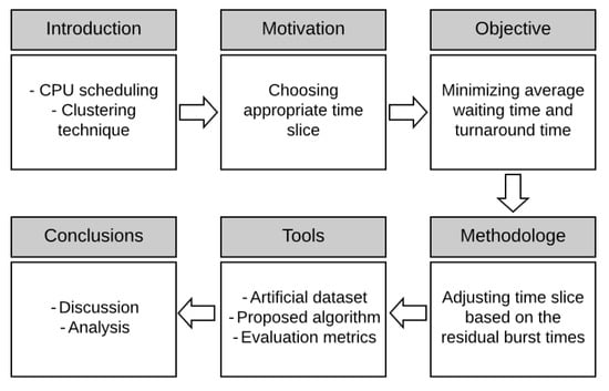
Figure 1.
Organization of the paper.
2. Related Works
For better CPU performance in most of the operating systems, the RR scheduling algorithm is widely implemented. Many variants of the RR algorithm have been proposed to minimize average waiting time and turnaround. This section discusses the most common versions of RR. Table 2 shows a comparison between the known versions of SRR.
Table 2.
Comparison of common versions of Round Robin (RR) (WT is acronym for waiting time, TT is acronym for turnaround time).
Aaron and Hong [32] proposed a dynamic version of SRR named Variable Time Round-Robin scheduling (VTRR). The time slice allocated to a process depends on the time needed to all tasks, process’s burst time, and number of processes in the ready queue.
Tarek and Abdelkader [33] proposed a weighting technique for SRR. The authors classified the processes into five weight categories based on their burst times. The weight of a process is inversely proportional to the weight; process with high weight receives more time slice and vice versa. Processes with burst time less than or equal to 10 tu receive 100% of the time slice defined by SRR, Processes with burst time less than or equal to 25 tu receive 80% of the time slice defined by SRR, and so on.
Samih et al. [18] proposed a dynamic version of SRR named Changeable Time Quantum (CTQ). Their algorithm finds the time slice that gives the smallest average waiting time at every round. CTQ calculates the average waiting time for a specific range of time slices and picks up the time slice corresponding to smallest average waiting time. Then, the processes in this round execute for this time slice.
Lipika [34] proposed a dynamic version of SRR by adjusting the time slice at the beginning of each round. The time slice is calculated depending on the remaining burst times in the subsequent rounds. In addition, the author also implemented SJF [35,36,37]. In SJF, the processes located in the ready queue are sorted in increasing order based on their burst times (i.e., the process having lowest burst time will be at the front of the ready queue and process having highest burst time will be at the end of the ready queue).
Christoph and Jeonghw [7] presented a dynamic version of SRR named Adaptive80 RR. The reason behind this name is that the time slice is set equal to process’s burst time at 80th percentile. Like Lipika’s [34], Adaptive80 RR sorts processes in increasing order. The time slice in each round depends on the processes located in the ready queue and if new process arrived, it will be added to the ready queue and will be considered in the subsequent calculations.
Samir et al. [38] proposed a hybrid scheduling algorithm based on SRR and SJF named SJF and RR with dynamic quantum (SRDQ). Their algorithm divided the ready queue into two subqueues Q1 and Q2; Q2 for long tasks (longer than the median) and Q1 for short tasks (shorter than the median). Like Adaptive80 RR [7] and Lipika’s [34] algorithms, this algorithm sorts the processes in ascending order in each subqueue. In every round, each process will be assigned a time slice depends on the median and the burst time of this process.
Samih [19] proposed a Proportional Weighted Round Robin (PWRR) as a modified version of SRR. PWRR assigns time slice to each process proportional to its burst time. Each process has a weight calculated by dividing its burst time by the summation of all burst times in the ready queue. Then the time slice is calculated depending on this weight.
Samih and Hirofumi [17] proposed a version of SRR named Adjustable Round Robin (ARR) that combines the low-scheduling overhead of SRR and favors a short process. ARR gives short process a chance, under predefined condition, to be executed until termination to minimize the average waiting time.
Uferah et al. [13] proposed a dynamic version of SRR named Amended Dynamic Round Robin (ADRR). The time slice is cyclically adjusted based on the process burst time. Like Adaptive80 RR [7], SRDQ [38] and Lipika’s [34] algorithms, ADRR sorts the processes in ascending order.
3. The Proposed Algorithm
The processes’ weights and numbers of allocation to the CPU (i.e., ) depend on the processes’ burst times , which are known, and are calculated as shown in the following subsections. We assumed that all processes arrive at the same time. The main advantage of the clustering technique in the proposed work is the ability to group similar processes in clusters. Similarity between processes depends on the values of and near each other, K-means algorithm is used for this purpose. The proposed technique consists of three stages: Data preparation, data clustering, and finally, dynamic time slice implementation.
3.1. Data Preparation
Data preparation stage consists of calculating and . The weight of the process, , is calculated from Equation (4):
where is the burst time of the process, and is the number of the processes in the ready queue. The number of context switches of the process, , is calculated from Equation (5):
where (standard time slice) is given by SRR, and denotes the largest integer smaller than or equal to . If the last round contains one process, this process will continue execution without switching its contents [4].
3.2. Data Clustering
Second stage comprises of two phases: First phase is finding the optimum number of clusters by using Silhouette method. A high average Silhouette width indicates a good clustering. Second phase is clustering the data into number resulted from Silhouette method by using K-means algorithm. In the proposed work, the clustering metrics are and
Each point is assigned to the closest centroid, and each combination of points assigned to the same centroid is a cluster. The assignment and updating steps are repeated until all centroids remain the same. To quantify the notion of “closest” for a specific data, the Euclidean distance is the proximity measure for data points in Euclidean space.
3.3. Dynamic Time Slice Implementation
In the third stage, dynamic time slice implementation, the weight of the cluster,, is calculated from Equation (6):
where is the average of burst times in the cluster. The time slice assigned to the cluster, , is calculated from Equation (7):
Each process in this cluster will execute for . In addition, a process that is close to its completion will get a chance to complete and leave the ready queue. A threshold is determined to allow the process that possesses burst time greater than STS and close to its completion to continue execution until termination. Therefore, the number of processes in the ready queue will be reduced by knocking out short processes relatively faster in the hope to minimize average waiting and turnaround times. The residual burst time of the process, , is calculated from Equation (8).
If a process satisfies the threshold condition, its equals zero and leaves the queue. When a new process arrived, it will be put at the tail of the queue to be scheduled in the next round. The clustering technique will be applied again for the survived processes (i.e., processes with or greater than the time slice assigned to them in the current round) and new processes (if arrived) in the next round. Figure 2 shows the flowchart of the proposed algorithm.
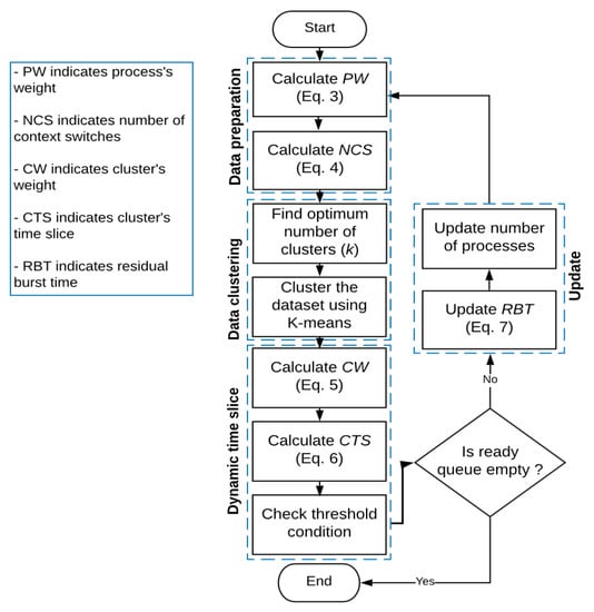
Figure 2.
Algorithm flowchart.
3.4. Illustrative Examples
The following examples provide a more in depth understanding of the proposed technique.
3.4.1. Example 1
From the benchmark datasets used in the experiments, the first dataset which contains 10 processes (see Table 3) will be used in this example. and are calculated from Equations (4) and (5), respectively. Silhouette method is used to find the optimum value of The location of a knee in the curve (see Figure 3) indicates the optimal number of clusters. From the curve, the optimal value of is 2.
Table 3.
Dataset_1.
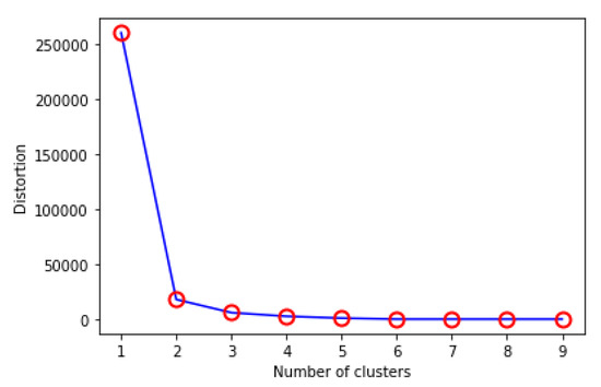
Figure 3.
Finding optimal number of clusters.
Now, will be used by K-means algorithm to clustering the data points. The 7th and 8th processes are grouped into cluster 1 and the others are grouped into cluster 0 (Table 4).
Table 4.
Clustered dataset_1.
The weight of cluster 0 equals 0.12271, and the weight of cluster 1 equals 0.87729. The time slice assigned to cluster 0 is 8.77287 tu, and the time slice assigned to cluster 1 is 1.227123 tu. The 7th and 8th processes will be assigned 1.227123 tu, and other processes will be assigned 1.227123 tu. The burst time of the third process is smaller than its cluster’s time slice, therefore it will terminate and leave. The number of processes, burst times, and weights will be updated for the next iteration and so forth until the ready queue becomes empty.
3.4.2. Example 2
Giving a short process more CPU time decreases the waiting time of this process more than it increases the waiting time of the long process. Consequently, the average waiting time decreases. To illustrate this concept, assume the following set of processes (Table 5) that arrive at the same time, each of which with its burst time, and the STS is 10 tu.
Table 5.
Four processes with the length of the burst time.
Using SRR scheduling, we would schedule these processes according to the following Gantt chart:

The waiting time is 30 tu for process P1, 10 tu for process P2, 42 tu for process P3, and 45 for process P4. Thus the average waiting time is 31.75 tu, and the average turnaround time is 50 tu. On the other hand, suppose that each process is assigned a percentile of STS equals as in Table 6.
Table 6.
Assigning time slice for the running processes in each round.
The results will be as shown in the following Gantt chart:

The waiting time is 20 tu for process P1, 7 tu for process P2, 42 tu for process P3, and 37 for process P4. Thus the average waiting time is 26.5 tu, and the average turnaround time is 44.75 tu.
4. Experimental Implementation
The experiments were carried out using a computer with the following specification: Intel core i5-2400 (3.10 GHz) processor, 16 GB memory, 1 TB HDD, Gnu/Linux Fedora 28 OS, and Python (Python 3.7.6 (default, Jan 8 2020, 20:23:39) [MSC v.1916 64 bit (AMD64)], and version of the notebook server is: 6.0.3).
4.1. Benchmark Datasets
Nine synthetic datasets are used to test the performance of the algorithms used in the comparison. Each dataset contains a number of processes used for numerical simulation. For each process of each dataset, the burst time is randomly generated. The datasets on hand vary in number of processes, processes’ burst times, processes’ weights, and processes’ number of context switches. Detailed information on datasets is presented in Table 7. Weight and NCS depend on the process’s burst time, which means that the most important variant of the benchmark dataset is the burst times of its processes.
Table 7.
Datasets specifications. The first column presents the dataset ID, the second column presents the number of processes in each dataset, the third column presents the number of attributes (i.e., BT, PW, and NCS), and the forth column presents the standard deviations.
4.2. Performance Evaluation
The proposed algorithm was compared with five common algorithms; PWRR, VTRR, BRR, SRR, and ADRR on different nine combinations of number of processes and burst times. The authors implemented all these algorithms using the benchmark datasets. The average waiting and turnaround times depend on the number of processes in the ready queue; as number of processes increases, time cost increases. In addition, long burst times of the processes increase the time cost. To emphasize the efficiency of the proposed algorithm, benchmark datasets varying in number and burst times of processes are used. The time taken in clustering the dataset is trivial. Comparing with waiting and turnaround times, it can be said that the clustering time has no effect and can be ignored. Table A1 compares between the running times of the proposed algorithm (including the times consumed in the clustering) against other methods.
Table A2 shows a comparison of the time cost between the proposed algorithm and other algorithms in terms of average waiting time, turnaround time, and NCS. Table A3, Figure 4, and Figure 5 show the superiority of the proposed algorithm over the compared algorithms in all the datasets where the time cost of the proposed algorithm is the smallest (average waiting time and average turnaround time are 979.14 tu, 1061.36 tu respectively). Figure 6 shows how much improvement is achieved by the proposed algorithm. Unlike PWRR, BRR, and SRR which their time slices are less than or equal to the time slice defined by SRR, VTRR may behave somewhat similar to FCFS as it may give a process very long time slice. Therefore, the time slices calculated in the VTRR algorithm are restricted to be less than or equal to the time slice defined by SRR (i.e., 10 tu).
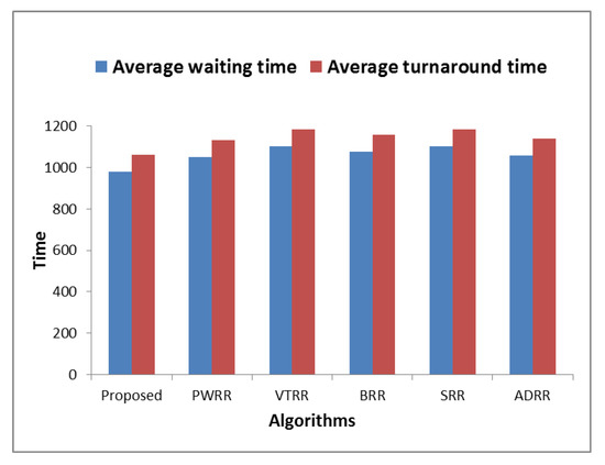
Figure 4.
Comparing algorithms’ time cost.
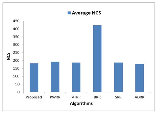
Figure 5.
Comparing algorithms’ NCS.
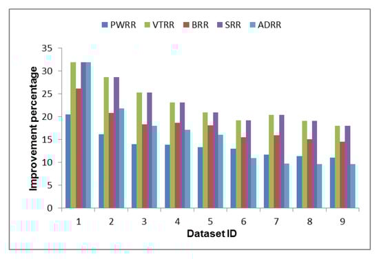
Figure 6.
Improvement percentage of the proposed algorithm over the compared algorithms.
5. Conclusions and Future Work
In this paper, a dynamic SRR-based CPU scheduling algorithm has been proposed that could be used in timesharing systems in which it is important to reduce the time cost of the scheduling. Unlike the SRR algorithm which uses fixed time slice for the processes in the ready queue in all rounds, the proposed algorithm uses dynamic time slice. The proposed algorithm benefits from clustering technique in grouping processes that resemble each other in their features (i.e., burst times, weights, and NCS). Each cluster is assigned a time slice proportional to its weight, and every process in this cluster receives this amount of time for its execution in the current round. The features will be updated in the subsequent rounds. In addition, the proposed algorithm gives processes that are close to completion a chance to complete execution and leave; this in turn helps in reducing number of processes in the ready queue and reducing NCS. The proposed algorithm was compared with five common algorithms from the point of view of average waiting, turnaround times, and NCS. The proposed algorithm outperformed all the others; however, it behaves somewhat similar to ADRR in NCS.
In cloud-computing systems, achieving optimality in scheduling processes over computing nodes is an important aim for all researchers interested in both cloud and scheduling, where the available resources must be scheduled using an efficient CPU scheduler to be assigned to clients. The relation between CSP (cloud service providers) and CSC (cloud service consumers) is formalized through service level agreement (SLA). CSP must achieve best performance through minimizing time cost. Because of the superiority of the proposed algorithm over the compared algorithms in all the datasets, the proposed algorithm in this work is promising for cloud computing systems.
Author Contributions
Conceptualization, formal analysis, methodology, and writing—original draft, S.M.M. The research work was carried out under the supervision of H.A. All authors have read and agreed to the published version of the manuscript.
Funding
This research received no external funding.
Acknowledgments
The authors thank the anonymous reviewers for their careful reading of our paper and their many insightful comments and suggestions.
Conflicts of Interest
The authors declare no conflict of interest.
Appendix A
Table A1.
Running times comparison between the proposed algorithm and five scheduling algorithms.
Table A1.
Running times comparison between the proposed algorithm and five scheduling algorithms.
| Dataset | Proposed | PWRR | VTRR | BRR | SRR | ADRR |
|---|---|---|---|---|---|---|
| 1 | 0.04 | 0.01 | 0.01 | 0.017 | 0.008 | 0.01 |
| 2 | 0.042 | 0.01 | 0.01 | 0.018 | 0.008 | 0.01 |
| 3 | 0.042 | 0.012 | 0.011 | 0.018 | 0.009 | 0.011 |
| 4 | 0.046 | 0.02 | 0.021 | 0.022 | 0.01 | 0.02 |
| 5 | 0.048 | 0.02 | 0.021 | 0.023 | 0.011 | 0.02 |
| 6 | 0.05 | 0.021 | 0.022 | 0.023 | 0.011 | 0.021 |
| 7 | 0.05 | 0.02 | 0.022 | 0.025 | 0.012 | 0.022 |
| 8 | 0.06 | 0.024 | 0.024 | 0.027 | 0.013 | 0.024 |
| 9 | 0.062 | 0.026 | 0.025 | 0.027 | 0.013 | 0.025 |
Table A2.
Average waiting time and turnaround time comparison between the proposed algorithm and five scheduling algorithms.
Table A2.
Average waiting time and turnaround time comparison between the proposed algorithm and five scheduling algorithms.
| Dataset | Proposed | PWRR | VTRR | BRR | SRR | ADRR | ||||||||||||
|---|---|---|---|---|---|---|---|---|---|---|---|---|---|---|---|---|---|---|
| WT | TT | NCS | WT | TT | NCS | WT | TT | NCS | WT | TT | NCS | WT | TT | NCS | WT | TT | NCS | |
| 1 | 398.41 | 538.61 | 124 | 450.85 | 591.05 | 141 | 485.90 | 626.10 | 124 | 467.60 | 607.80 | 306 | 485.90 | 626.10 | 124 | 485.9 | 626.1 | 124 |
| 2 | 552.37 | 660.44 | 140 | 605.22 | 713.28 | 154 | 653.27 | 761.33 | 144 | 622.20 | 730.27 | 341 | 653.27 | 761.33 | 144 | 625.933 | 734 | 139 |
| 3 | 704.30 | 795.40 | 156 | 760.63 | 851.73 | 169 | 812.35 | 903.45 | 160 | 779.50 | 870.60 | 371 | 812.35 | 903.45 | 160 | 778.3 | 869.4 | 154 |
| 4 | 852.07 | 932.59 | 171 | 918.54 | 999.06 | 182 | 968.24 | 1048.76 | 175 | 943.52 | 1024.04 | 401 | 968.24 | 1048.76 | 175 | 935.36 | 1015.88 | 169 |
| 5 | 1004.37 | 1077.63 | 185 | 1078.26 | 1151.53 | 195 | 1125.67 | 1198.93 | 190 | 1107.80 | 1181.07 | 430 | 1125.67 | 1198.93 | 190 | 1094.77 | 1168.03 | 184 |
| 6 | 1154.23 | 1222.00 | 199 | 1236.42 | 1304.20 | 210 | 1280.57 | 1348.34 | 205 | 1254.31 | 1322.09 | 455 | 1280.57 | 1348.34 | 205 | 1222.97 | 1290.74 | 194 |
| 7 | 1275.34 | 1338.61 | 210 | 1356.38 | 1419.65 | 220 | 1423.53 | 1486.80 | 219 | 1388.58 | 1451.85 | 479 | 1423.53 | 1486.80 | 219 | 1341.85 | 1405.13 | 204 |
| 8 | 1383.72 | 1443.23 | 221 | 1468.75 | 1528.26 | 230 | 1533.09 | 1592.60 | 229 | 1498.91 | 1558.42 | 499 | 1533.09 | 1592.60 | 229 | 1454.76 | 1514.27 | 214 |
| 9 | 1487.44 | 1543.74 | 228 | 1575.99 | 1632.29 | 238 | 1637.48 | 1693.78 | 239 | 1605.92 | 1662.22 | 519 | 1637.48 | 1693.78 | 239 | 1563.62 | 1619.92 | 224 |
| Average | 979.14 | 1061.36 | 181.56 | 1050.11 | 1132.34 | 193.22 | 1102.23 | 1184.45 | 187.22 | 1074.26 | 1156.48 | 422.33 | 1102.23 | 1184.45 | 187.22 | 1055.94 | 1138.16 | 178.44 |
| Improvement% | 6.76 | 6.27 | 5.87 | 11.17 | 10.39 | 2.85 | 8.85 | 8.23 | 56.93 | 11.17 | 10.39 | 2.85 | 7.27 | 6.75 | −1.74 | |||
Table A3.
Improvement percentages of the proposed algorithm over five scheduling algorithms.
Table A3.
Improvement percentages of the proposed algorithm over five scheduling algorithms.
| PWRR | VTRR | BRR | SRR | ADRR | |||||||||||
|---|---|---|---|---|---|---|---|---|---|---|---|---|---|---|---|
| WT | TT | NCS | WT | TT | NCS | WT | TT | NCS | WT | TT | NCS | WT | TT | NCS | |
| 1 | 11.63 | 8.87 | 12.06 | 18.01 | 13.97 | 0.00 | 14.80 | 11.38 | 59.48 | 18.01 | 13.97 | 0.00 | 18.01 | 13.97 | 0.00 |
| 2 | 8.73 | 7.41 | 9.09 | 15.45 | 13.25 | 2.78 | 11.22 | 9.56 | 58.94 | 15.45 | 13.25 | 2.78 | 11.75 | 10.02 | −0.72 |
| 3 | 7.41 | 6.61 | 7.69 | 13.30 | 11.96 | 2.50 | 9.65 | 8.64 | 57.95 | 13.30 | 11.96 | 2.50 | 9.51 | 8.51 | −1.30 |
| 4 | 7.24 | 6.65 | 6.04 | 12.00 | 11.08 | 2.29 | 9.69 | 8.93 | 57.36 | 12.00 | 11.08 | 2.29 | 8.90 | 8.20 | −1.18 |
| 5 | 6.85 | 6.42 | 5.13 | 10.78 | 10.12 | 2.63 | 9.34 | 8.76 | 56.98 | 10.78 | 10.12 | 2.63 | 8.26 | 7.74 | −0.54 |
| 6 | 6.65 | 6.30 | 5.24 | 9.87 | 9.37 | 2.93 | 7.98 | 7.57 | 56.26 | 9.87 | 9.37 | 2.93 | 5.62 | 5.33 | −2.58 |
| 7 | 5.97 | 5.71 | 4.55 | 10.41 | 9.97 | 4.11 | 8.16 | 7.80 | 56.16 | 10.41 | 9.97 | 4.11 | 4.96 | 4.73 | −2.94 |
| 8 | 5.79 | 5.56 | 3.91 | 9.74 | 9.38 | 3.49 | 7.68 | 7.39 | 55.71 | 9.74 | 9.38 | 3.49 | 4.88 | 4.69 | −3.27 |
| 9 | 5.62 | 5.42 | 4.20 | 9.16 | 8.86 | 4.60 | 7.38 | 7.13 | 56.07 | 9.16 | 8.86 | 4.60 | 4.87 | 4.70 | −1.79 |
References
- Chandiramani, K.; Verma, R.; Sivagami, M. A Modified Priority Preemptive Algorithm for CPU Scheduling. Procedia Comput. Sci. 2019, 165, 363–369. [Google Scholar] [CrossRef]
- Rajput, I.S.; Gupta, D. A Priority based Round Robin CPU Scheduling Algorithm for Real Time Systems. J. Adv. Eng. Technol. 2012, 1, 1–11. [Google Scholar]
- Reddy, M.R.; Ganesh, V.; Lakshmi, S.; Sireesha, Y. Comparative Analysis of CPU Scheduling Algorithms and Their Optimal Solutions. In Proceedings of the 2019 3rd International Conference on Computing Methodologies and Communication (ICCMC), Erode, India, 27–29 March 2019; pp. 255–260. [Google Scholar] [CrossRef]
- Silberschatz, A.; Galvin, P.B.; Gagne, G. Operating System Concepts, 10th ed.; Wiley Publ.: Hoboken, NJ, USA, 2018. [Google Scholar]
- Sunil, J.G.; Anisha Gnana, V.T.; Karthija, V. Fundamentals of Operating Systems Concepts; Lambert Academic Publications: Saarbrucken, Germany, 2018. [Google Scholar]
- Silberschatz, A.; Gagne, G.B.; Galvin, P. Operating Systems Concepts, 9th ed.; Wiley Publ.: Hoboken, NJ, USA, 2012. [Google Scholar]
- McGuire, C.; Lee, J. The Adaptive80 Round Robin Scheduling Algorithm. Trans. Eng. Technol. 2015, 243–258. [Google Scholar]
- Wilmshurst, T. Designing Embedded Systems with PIC Microcontrollers; Elsevier BV: Amsterdam, The Netherlands, 2010. [Google Scholar]
- Singh, P.; Pandey, A.; Mekonnen, A. Varying Response Ratio Priority: A Preemptive CPU Scheduling Algorithm (VRRP). J. Comput. Commun. 2015, 3, 40–51. [Google Scholar] [CrossRef][Green Version]
- Farooq, M.U.; Shakoor, A.; Siddique, A.B. An Efficient Dynamic Round Robin algorithm for CPU scheduling. In Proceedings of the 2017 International Conference on Communication, Computing and Digital Systems (C-CODE), Islamabad, Pakistan, 8–9 March 2017; 2017; pp. 244–248. [Google Scholar] [CrossRef]
- Alsulami, A.A.; Abu Al-Haija, Q.; Thanoon, M.I.; Mao, Q. Performance Evaluation of Dynamic Round Robin Algorithms for CPU Scheduling. In Proceedings of the 2019 SoutheastCon, Huntsville, AL, USA, 11–14 April 2019; pp. 1–5. [Google Scholar]
- Singh, A.; Goyal, P.; Batra, S. An optimized round robin scheduling algorithm for CPU scheduling. Int. J. Comput. Sci. Eng. 2010, 2, 2383–2385. [Google Scholar]
- Shafi, U.; Shah, M.; Wahid, A.; Abbasi, K.; Javaid, Q.; Asghar, M.; Haider, M. A Novel Amended Dynamic Round Robin Scheduling Algorithm for Timeshared Systems. Int. Arab. J. Inf. Technol. 2019, 17, 90–98. [Google Scholar] [CrossRef]
- Garrido, J.M. Performance Modeling of Operating Systems Using Object-Oriented Simulation, 1st ed.; Series in Computer Science; Springer US: New York, NY, USA, 2002. [Google Scholar]
- Tajwar, M.M.; Pathan, N.; Hussaini, L.; Abubakar, A. CPU Scheduling with a Round Robin Algorithm Based on an Effective Time Slice. J. Inf. Process. Syst. 2017, 13, 941–950. [Google Scholar] [CrossRef]
- Saidu, I.; Subramaniam, S.; Jaafar, A.; Zukarnain, Z.A. Open Access A load-aware weighted round-robin algorithm for IEEE 802. 16 networks. EURASIP J. Wirel. Commun. Netw. 2014, 1–12. [Google Scholar]
- Mostafa, S.M.; Amano, H. An Adjustable Round Robin Scheduling Algorithm in Interactive Systems. Inf. Eng. Express 2019, 5, 11–18. [Google Scholar]
- Mostafa, S.M.; Rida, S.Z.; Hamad, S.H. Finding Time Quantum of Round Robin CPU Scheduling Algorithm in General Computing Systems Using Integer Programming. Int. J. New Comput. Archit. Appl. 2010, 5, 64–71. [Google Scholar]
- Mostafa, S.M. Proportional Weighted Round Robin: A Proportional Share CPU Scheduler in Time Sharing Systems. Int. J. New Comput. Arch. Appl. 2018, 8, 142–147. [Google Scholar] [CrossRef]
- Lasek, P.; Gryz, J. Density-based clustering with constraints. Comput. Sci. Inf. Syst. 2019, 16, 469–489. [Google Scholar] [CrossRef]
- Lengyel, A.; Botta-Dukát, Z. Silhouette width using generalized mean—A flexible method for assessing clustering efficiency. Ecol. Evol. 2019, 9, 13231–13243. [Google Scholar] [CrossRef] [PubMed]
- Starczewski, A.; Krzyżak, A. Performance Evaluation of the Silhouette Index BT. In Artificial Intelligence and Soft Computing; Lecture Notes in Computer Science; Springer: Cham, Switzerland, 2015; Volume 9120, pp. 49–58. [Google Scholar]
- Al-Dhaafri, H.; Alosani, M. Closing the strategic planning and implementation gap through excellence in the public sector: Empirical investigation using SEM. Meas. Bus. Excel. 2020, 35–47. [Google Scholar] [CrossRef]
- Xu, D.; Tian, Y. A Comprehensive Survey of Clustering Algorithms. Ann. Data Sci. 2015, 2, 165–193. [Google Scholar] [CrossRef]
- Wu, J. Cluster Analysis and K-means Clustering: An Introduction; Springer Science and Business Media LLC: Berlin, Germany, 2012; pp. 1–16. [Google Scholar]
- Yuan, C.; Yang, H. Research on K-Value Selection Method of K-Means Clustering Algorithm. J. Multidiscip. Sci. J. 2019, 2, 16. [Google Scholar] [CrossRef]
- Guan, C.; Yuen, K.K.F.; Coenen, F. Particle swarm Optimized Density-based Clustering and Classification: Supervised and unsupervised learning approaches. Swarm Evol. Comput. 2019, 44, 876–896. [Google Scholar] [CrossRef]
- Mostafa, S.M.; Amano, H. Effect of clustering data in improving machine learning model accuracy. J. Theor. Appl. Inf. Technol. 2019, 97, 2973–2981. [Google Scholar]
- Kassambara, A. Practical Guide to Cluster Analysis in R: Unsupervised Machine Learning; CreateSpace Independent Publishing Platform: Scotts Valley, CA, USA, 2017. [Google Scholar]
- Inyang, U.G.; Obot, O.O.; Ekpenyong, M.E.; Bolanle, A.M. Unsupervised Learning Framework for Customer Requisition and Behavioral Pattern Classification. Mod. Appl. Sci. 2017, 11, 151. [Google Scholar] [CrossRef][Green Version]
- Liu, Y.; Li, Z.; Xiong, H.; Gao, X.; Wu, J. Understanding of Internal Clustering Validation Measures. In Proceedings of the 2010 IEEE International Conference on Data Mining, Sydney, Australia, 13–17 December 2010; Institute of Electrical and Electronics Engineers (IEEE): Sydney, Australia; pp. 911–916. [Google Scholar]
- Harwood, A.; Shen, H. Using fundamental electrical theory for varying time quantum uni-processor scheduling. J. Syst. Arch. 2001, 47, 181–192. [Google Scholar] [CrossRef]
- Helmy, T. Burst Round Robin as a Proportional-Share Scheduling Algorithm. Proceedings of The Fourth IEEE-GCC Conference on Towards Techno-Industrial Innovations, Bahrain, Manama, 11–14 November 2007; pp. 424–428. [Google Scholar]
- Datta, L. Efficient Round Robin Scheduling Algorithm with Dynamic Time Slice. Int. J. Educ. Manag. Eng. 2015, 5, 10–19. [Google Scholar] [CrossRef]
- Zouaoui, S.; Boussaid, L.; Mtibaa, A. Improved time quantum length estimation for round robin scheduling algorithm using neural network. Indones. J. Electr. Eng. Inform. 2019, 7, 190–202. [Google Scholar]
- Pandey, A.; Singh, P.; Gebreegziabher, N.H.; Kemal, A. Chronically Evaluated Highest Instantaneous Priority Next: A Novel Algorithm for Processor Scheduling. J. Comput. Commun. 2016, 4, 146–159. [Google Scholar] [CrossRef][Green Version]
- Srinivasu, N.; Balakrishna, A.S.V.; Lakshmi, R.D. An Augmented Dynamic Round Robin CPU. J. Theor. Appl. Inf. Technol. 2015, 76. [Google Scholar]
- El Mougy, S.; Sarhan, S.; Joundy, M. A novel hybrid of Shortest job first and round Robin with dynamic variable quantum time task scheduling technique. J. Cloud Comput. 2017, 6, 1–12. [Google Scholar] [CrossRef]


© 2020 by the authors. Licensee MDPI, Basel, Switzerland. This article is an open access article distributed under the terms and conditions of the Creative Commons Attribution (CC BY) license (http://creativecommons.org/licenses/by/4.0/).