CFD Simulation of a Temperature Control System for Galvanizing Line of Metal Band Based on Jet Cooling Heat Transfer


Abstract
:1. Introduction
2. Numerical Simulations on Jet Impingement
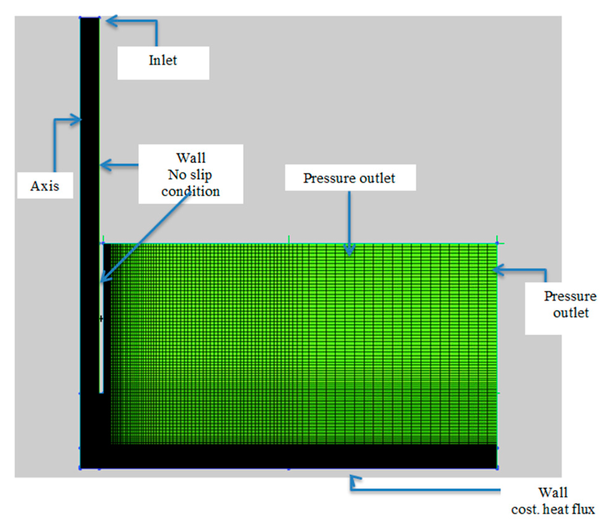
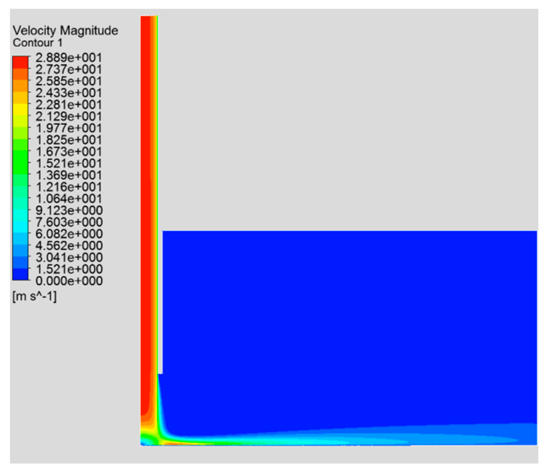
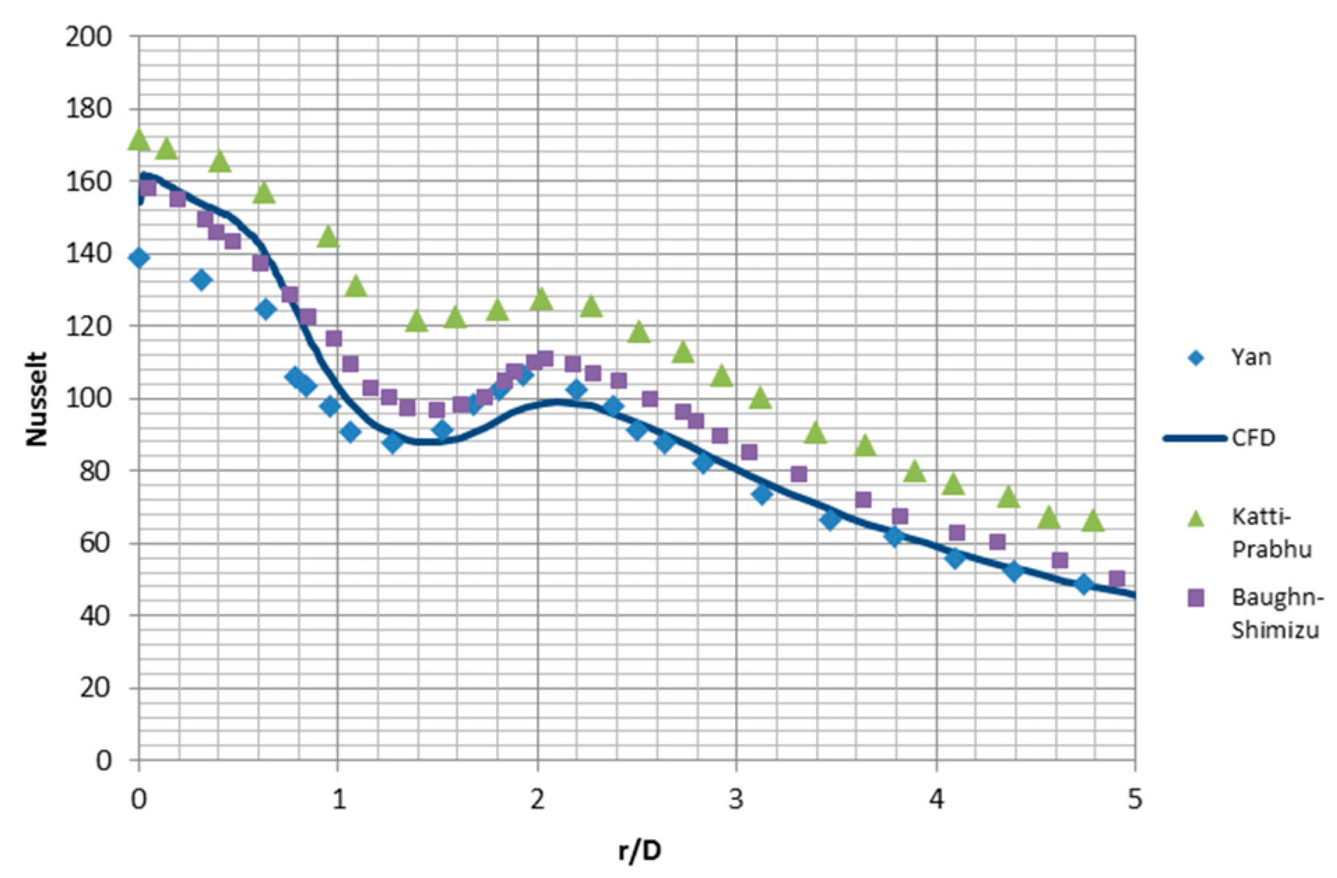
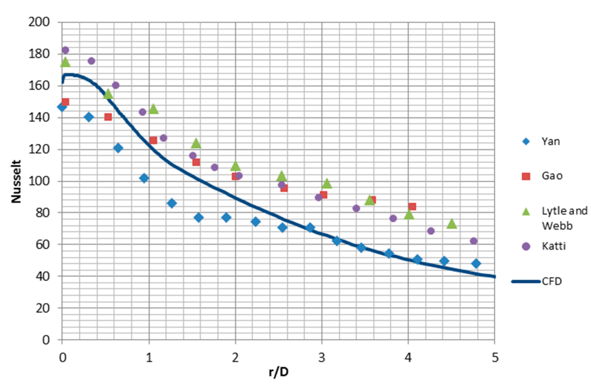
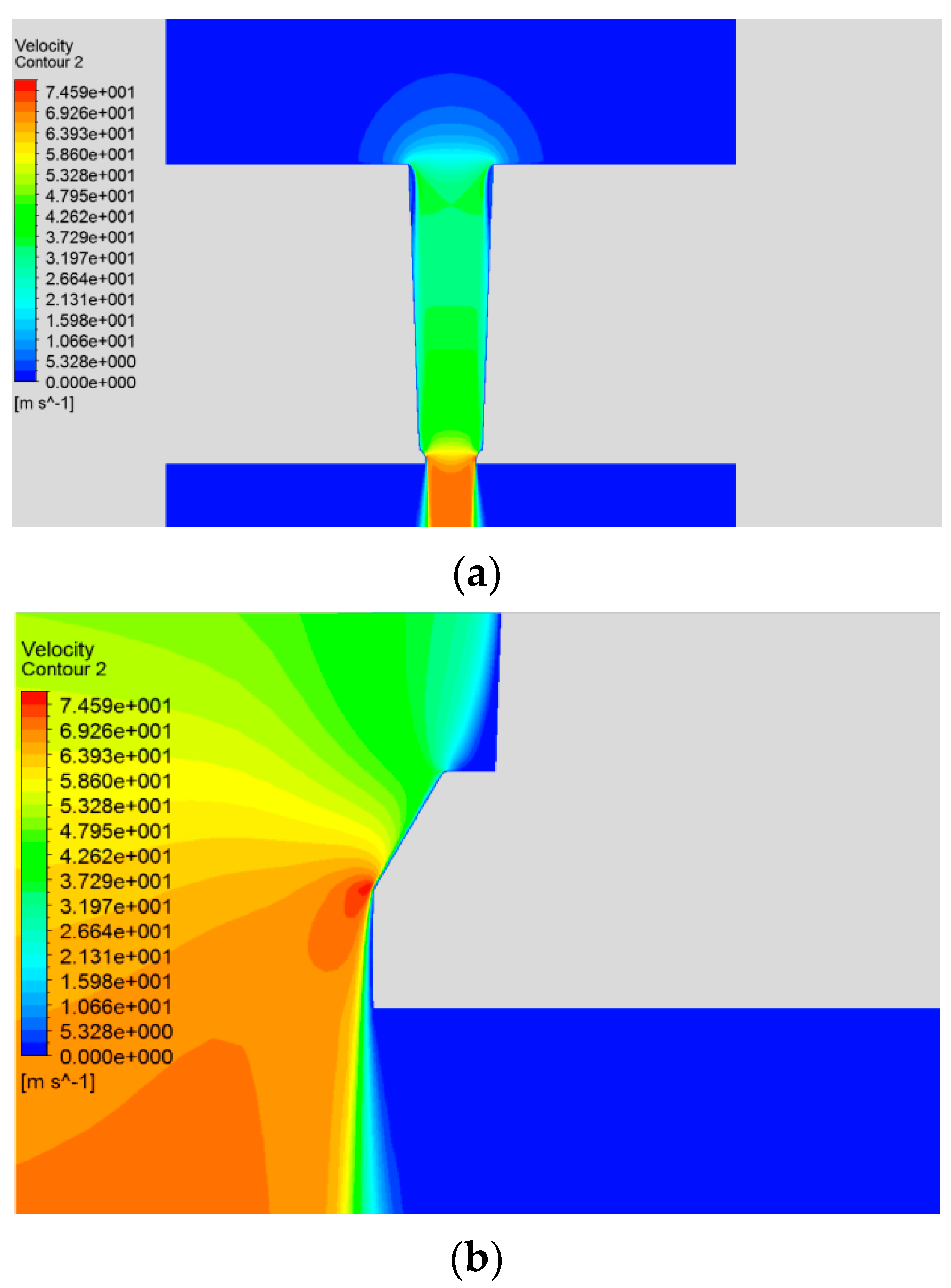
2.1. Axisymmetric 2D Model
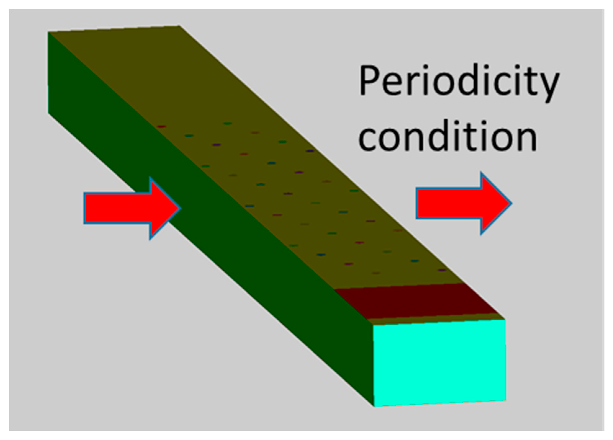
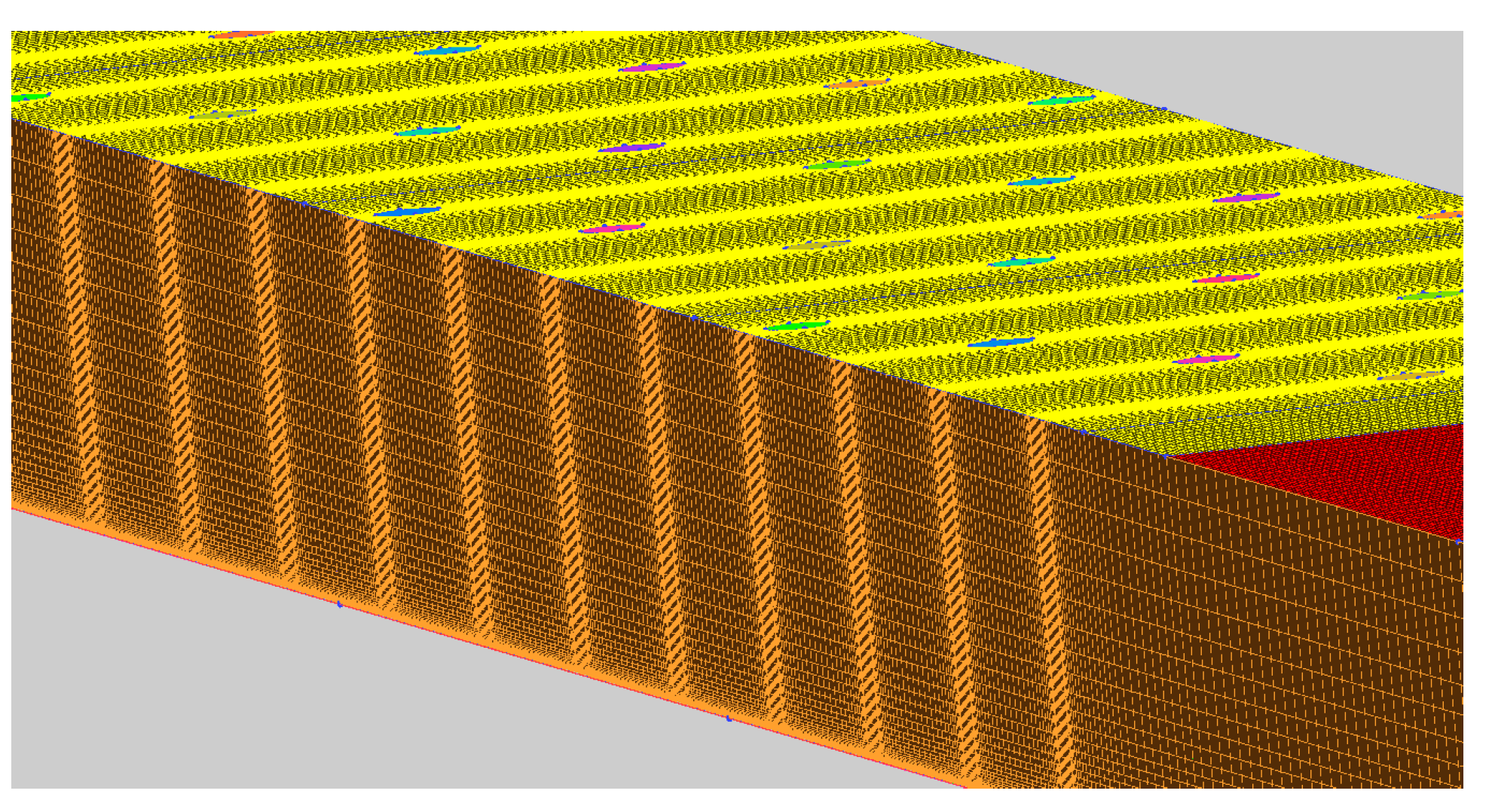
2.2. 3D Model
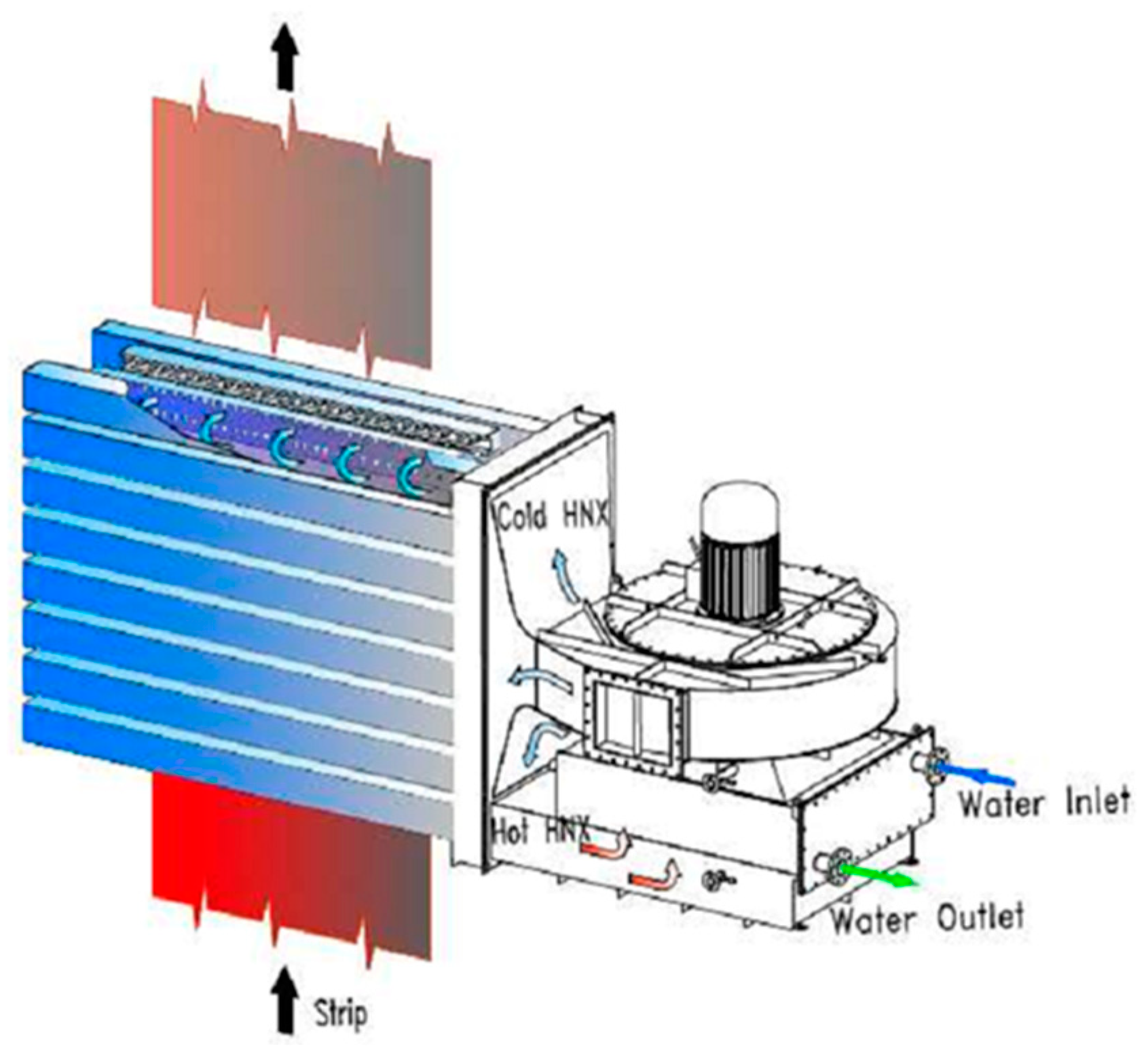
3. Industrial Jet Cooler Module
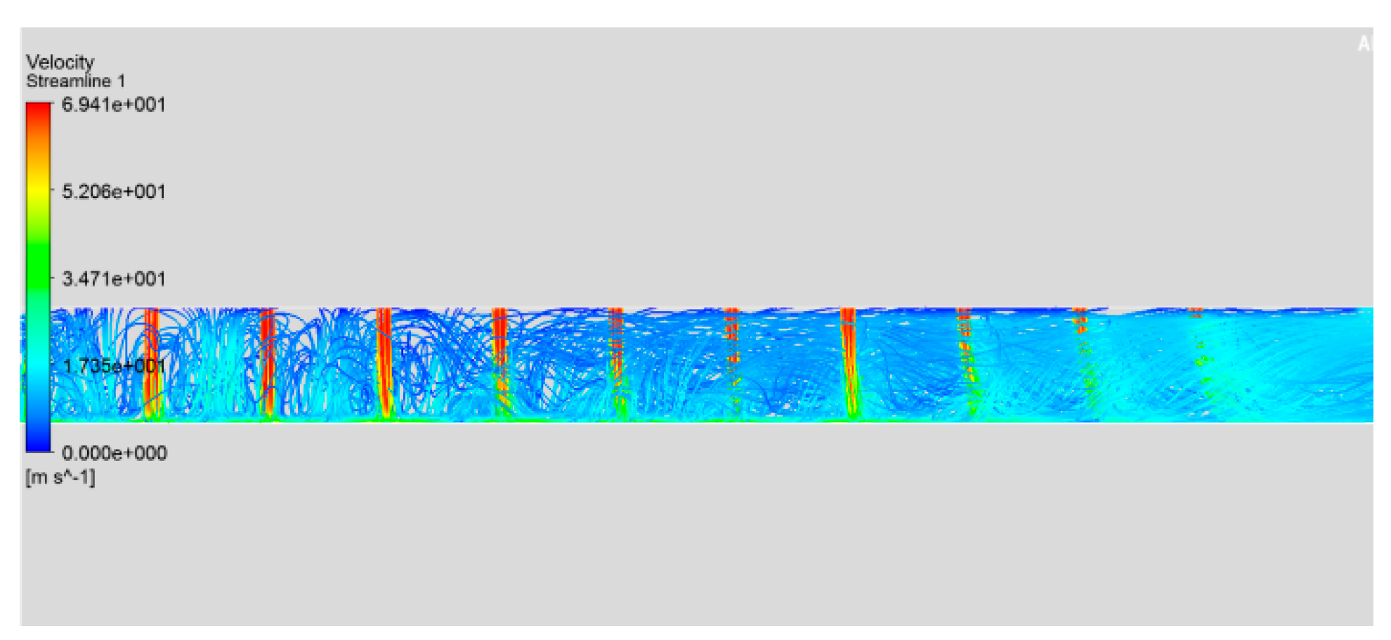
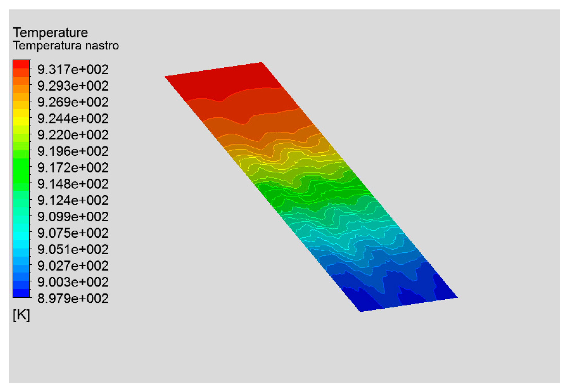
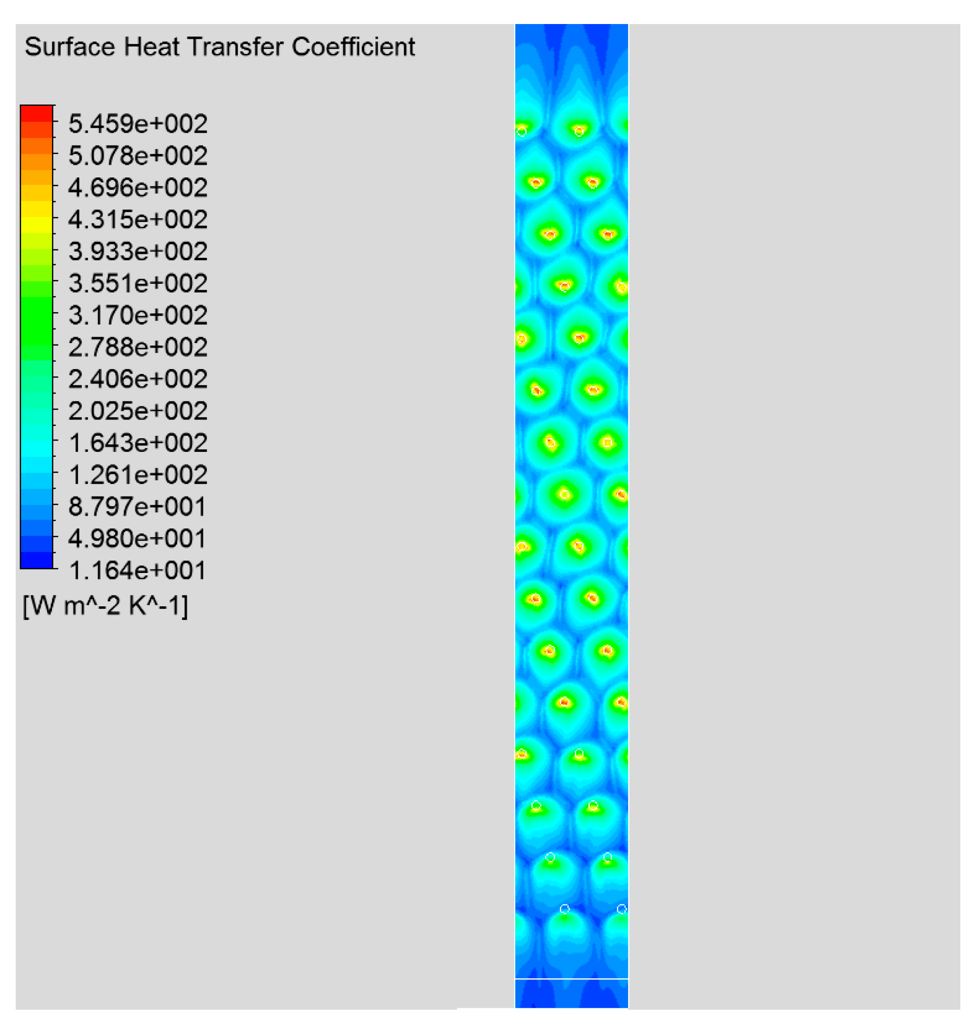
3.1. CFD Simulation of the Module
3.2. Heat Coefficient from Correlations and CFD
4. Conclusions
- -
- to calibrate the heat transfer correlations available in the literature for the specific industrial design layout;
- -
- to give a detailed insight into the jet impingement mechanism in the system in order to optimize the heat transfer and reduce, if possible, the mass flow rate of the cooling fluid.
Author Contributions
Funding
Acknowledgments
Conflicts of Interest
References
- Basso, D.; Cravero, C.; Reverberi, A.P.; Fabiano, B. CFD analysis of regenerative chambers for energy efficiency improvement in glass production plants. Energies 2015, 88945–88961. [Google Scholar] [CrossRef] [Green Version]
- Cogliandro, S.; Cravero, C.; Marini, M.; Spoladore, A. Simulation strategies for regenerative chambers in glass production plants with strategic exhaust gas recirculation system. IIETA Int. J. Heat Technol. 2017, 35, S449–S455. [Google Scholar] [CrossRef]
- Cravero, C.; de Domenico, D.; Leutcha, P.J.; Marsano, D. Strategies for the numerical modelling of regenerative pre-heating systems for recycled glass raw material, mathematical modelling of engineering problems. IETA 2019, 6, 324–332. Available online: http://iieta.org/journals/mmep (accessed on 28 July 2020). [CrossRef] [Green Version]
- Cravero, C.; Satta, A. Comparison of semi empirical correlations and a navier-stokes method for the overall performance assessment of turbine cascades. ASME J. Fluids Eng. 2003, 125, 308–314. [Google Scholar] [CrossRef]
- Cravero, C.; Satta, A. A CFD model for real gas flows, ASME Paper 2000-GT-0518. In Proceedings of the ASME Turbo Expo 2000, Munich, Germany, 8–11 May 2000. [Google Scholar]
- Zuckerman, N.; Lior, N. Jet impingement heat transfer: Physics, correlations and numerical modeling. Adv. Heat Transf. 2006, 39, 566–630. [Google Scholar]
- Katti, V.; Prabhu, S.V. Experimental study and theoretical analysis of local heat transfer distribution between smooth flat surface and impinging air jet from a circular straight pipe nozzle. J. Heat Mass Transf. 2008, 51, 4480–4495. [Google Scholar] [CrossRef]
- Geers, L.F.G. Multiple Impinging Jet Arrays: An Experimental Study on Flow and Heat Transfer. Ph.D. Thesis, Delft University of Technology, Delft, The Netherlands, 2004. [Google Scholar]
- Behnia, M.; Parneix, S.; Durbin, P.A. Prediction of heat transfer in an axisymmetric turbulent jet impinging on a flat plate. Int. J. Heat Mass Transf. 1998, 41, 1845–1855. [Google Scholar] [CrossRef]
- Bovo, M.; Etemad, S.; Davidson, L. On the numerical modeling of impinging jet heat transfer. In Proceedings of the International Symposium. on Convective Heat and Mass Transfer in Sustainable Energy, Yasmine Hammamet, Tunisia, 26 April–1 May 2009. [Google Scholar]
- Thielen, L. Modeling and Calculation of Flow and Heat Transfer in Multiple Impinging Jets. Ph.D. Thesis, Delft University of Technology, Delft, The Netherlands, 2003. [Google Scholar]
- Pattamatta, A.; Singh, G.; Mongia, H. Assessment of turbulence models for free and confined impinging jet flows. In Proceedings of the 42nd Thermophysics Conference, Honolulu, HI, USA, 27–30 June 2011. [Google Scholar]
- Chougule, N.K.; Parishwad, G.V.; Gore, P.R.; Pagnis, S.; Sapali, S.N. CFD analysis of multi-jet air impingement on flat plate. In Proceedings of the World Congress on Engineering, London, UK, 6–8 July 2011; Volume 3. [Google Scholar]
- Wae-Hayee, M.; Perapong, T.; Nuntadusit, C. Influence of nozzle arrangement on flow and heat transfer characteristics of arrays of circular impinging jets. Songklanakarin J. Sci. Technol. 2013, 35, 203–212. [Google Scholar]
- ERCOFTAC. Classic Database, Normally-Impinging Jet from a Circular Nozzle. Available online: www.ercoftac.org (accessed on 28 July 2020).
- ERCOFTAC. Database, Multiple-impinging jets: Flow and heat transfer—Test case 11.4. In Proceedings of the 11th Workshop at Chalmers University of Technology, Gothenburg, Sweden, 7–8 April 2005. [Google Scholar]
- Yan, X. A Preheated-Wall Transient Method Using Liquid Crystals for the Measurement of Heat Transfer on External Surfaces and in Ducts. Ph.D. Thesis, University of California, Davis, CA, USA, 1993. [Google Scholar]
- Baughn, J.W.; Shimizu, S. Heat transfer measurement from a surface with uniform heat flux and impinging jet. ASME J. Heat Transf. 1989, 111, 1096–1098. [Google Scholar] [CrossRef]
- Milani, A. Sviluppo Tecnologico dei Forni Continui per i Trattamenti Termici, Scambio Termico per Convezione Nei “Jet-Coolers”; Internal Report; Danieli Spa: Buttrio, Italy, 2003. [Google Scholar]


| Nu (Average) | Convective Heat Transfer Coefficient h [W/m2 K] | Percentage Error | |
|---|---|---|---|
| Geers—exp | 83.13 | 165.18 | --- |
| CFD | 92.20 | 183.19 | 10.90 |
| Correlations | |||
| Geers (inlet) | 81.20 | 161.39 | −2.29 |
| Milani (film) | 289.58 | 158.88 | −3.82 |
| Floreschutz (film) | 97.03 | 192.79 | 16.70 |
| Huber-Viskanta (inlet) | 90.01 | 178.84 | 8.27 |
| Huber-Viskanta (film) | 73.38 | 145.80 | −11.73 |
| Goldstein-Seol (inlet) | 51.56 | 102.45 | −37.97 |
| Goldstein-Seol (film) | 42.16 | 83.77 | −49.29 |
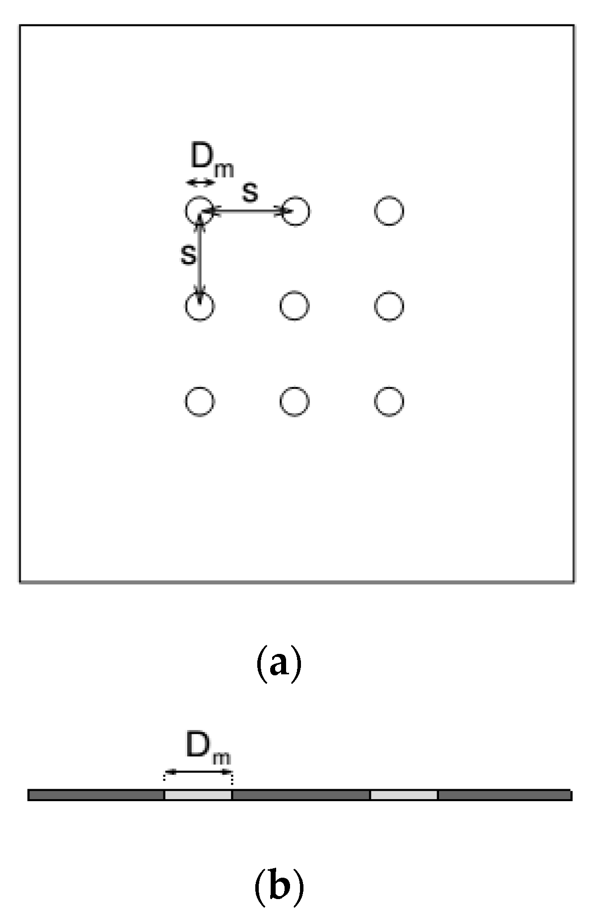
| H/D | 6.250 |
| (pjet/D)spanwise | 6.875 |
| (pjet/D)streamwise | 6.250 |
| Band thickness [mm] | 0.680 |
| Nu (Average) | Convective Heat Transfer Coefficient h [W/m2 K] | Percentage Error | |
|---|---|---|---|
| CFD | 83.39 | 171.31 | ---- |
| Geers (inlet) | 102.25 | 210.06 | 22.61 |
| Milani (film) | 339.55 | 165.92 | −3.15 |
| Floreschutz (film) | 53.14 | 178.51 | 4.20 |
| Martin (film) | 46.65 | 156.72 | −8.25 |
| Huber-Viskanta (inlet) | 99.71 | 204.85 | 19.57 |
| Huber-Viskanta (film) | 49.18 | 165.22 | −3.55 |
| Goldstein-Seol (inlet) | 41.30 | 84.84 | −50.47 |
| Goldstein-Seol (film) | 20.57 | 69.12 | −59.65 |
© 2020 by the authors. Licensee MDPI, Basel, Switzerland. This article is an open access article distributed under the terms and conditions of the Creative Commons Attribution (CC BY) license (http://creativecommons.org/licenses/by/4.0/).
Share and Cite
Carozzo, G.; Cravero, C.; Marini, M.; Mazza, M. CFD Simulation of a Temperature Control System for Galvanizing Line of Metal Band Based on Jet Cooling Heat Transfer. Appl. Sci. 2020, 10, 5248. https://doi.org/10.3390/app10155248
Carozzo G, Cravero C, Marini M, Mazza M. CFD Simulation of a Temperature Control System for Galvanizing Line of Metal Band Based on Jet Cooling Heat Transfer. Applied Sciences. 2020; 10(15):5248. https://doi.org/10.3390/app10155248
Chicago/Turabian StyleCarozzo, Giovanni, Carlo Cravero, Martino Marini, and Matteo Mazza. 2020. "CFD Simulation of a Temperature Control System for Galvanizing Line of Metal Band Based on Jet Cooling Heat Transfer" Applied Sciences 10, no. 15: 5248. https://doi.org/10.3390/app10155248