Abstract
The design of a V-belt continuously variable transmission (CVT) system is a complex problem due to the multiple interactions between components during its operation. Literature on CVT system design methods is scarce, and the vast majority of works include implicit equations that hinder applications at a basic design level. This research aims to introduce a numerical CVT design method for electric vehicles (EV) and internal combustion engine (ICE) vehicles considering each one of their components and using mechanical centrifugal actuators and a rubber V-belt. This design method is based on user needs, for which there are three main requirements: road specifications, vehicle characteristics, and expected performance. This method is focused on a transmission for a vehicle traveling on the same route constantly, such as public transport vehicles. From three-wheelers to medium cargo vehicles, there is a greatly diverse range of potential applications for using this method for each type of standard rubber V-belt.
1. Introduction
The implementation of continuously variable transmission (CVT) systems in transport vehicles has been growing during the last decades [1,2] due to the inherent advantages of using this type of transmission [3]. CVTs offer the option of continuously varying their speed ratio over a wide range of angular speeds, allowing for an infinite number of ratios to be obtained [4,5]. CVT transmissions in vehicles achieve lower values of polluting gases emissions [6,7,8], involve smaller parts, weigh less, and allow for better energy performance when compared to gearboxes [3,9]. These systems allow engine operation to be sustained at maximum efficiency, which improves energy consumption and enhances driving comfort either in electric vehicles (EV), internal combustion engine (ICE) vehicles, and hybrid vehicles [10,11]. Although CVTs have relatively low local efficiency compared to traditional vehicle transmissions [5], when operating in conjunction with an engine or motor, the system’s overall efficiency increases, due to CVTs operating more frequently in the regions of higher engine/motor efficiency [10,12,13]. The following articles present a component-based approach to address the design of this type of transmission. A taxonomic description of the most sensitive research in the field of CVT design is presented below.
Certain parameters such as clamping force, slip between pulleys, torque load, and many others must be considered when designing a CVT, because the interactions between them affects the operation, efficiency, and conceptualization of the system [5,14,15,16]. The belt is the main component responsible for developing and interacting with the mentioned forces. Therefore, authors such as Kim et al. in [4] described a formula to easily determine the axial forces present in a rubber V-belt CVT with assumptions such as a negligible slip angle in the driven pulley active area and a constant belt tension on the driver pulley with an accuracy of 5%. Furthermore, they found that when it is desired to maintain a constant speed, the driver pulley axial force has a linear behavior against the increased system torque load. In [17], the authors compare three analytical rubber V-belt models; the Kim–Kim model, the Dittrich model, and the Cammalleri model, where the most sensitive results indicate that the Kim–Kim model describes the CVT transmission working accurately based on the experimental data. Other researchers such as Asayama et al. [18] developed an analytical model of metal belts behavior, in order to specify the variations on belt tension that take place when operating CVT. The study also allows the method to determine the clamping force under certain conditions, and thus determine the required pressure to prevent slippage on the belt. The efficiency of the CVT systems depends on the required clamping force values and the belt slip. Regarding the latter, in research by [19,20] the authors use metal V-belts and argue that the belt slip depends on the driven pulley capacity to transmit torque; considering a relation between torque, clamping force, the friction coefficient between the pulleys and the belt, and the speed ratio. In the operation of the metal belts CVT system, the metal belt passes through the idle sector of the pulley, a gap is generated between the members, generating a micro-slip and thus causing a loss in the torque transmission [14]. At low speed ratios this type of belt adds power transmission to the system, but at high ratios this capacity decreases [2]. Furthermore, the efficiency of a CVT decreases against high values of clamping force [21]. In chain CVT systems, the chain pins and the pulley plates are in contact. This interaction provides the power transmission from the driver pulley to the driven pulley. This leads to impacts when the chain pins and links pass in and out of the pulleys [2]. Although the belt is an important element in the design of the CVT, there are also other crucial elements that allow the change of the speed ratio and interaction with the belt.
The CVTs speed ratio actuation and control are given by a variety of mechanisms present on the pulleys. The actuators design has been an important matter discussed by different authors. Cammalleri [22] presents a model to design the mechanical actuators for the driver and driven pulleys, being the actuators, respectively, a centrifugal roller and a helical torque cam with a compression torsion spring. The model presented allows calculation of the torque required by the system to be kept as close as possible to that provided by the engine/motor, thus increasing efficiency. The latter mechanisms are usually installed in low-powered vehicles. Complementing the above, different authors present models, designs and control strategies of these systems that allow pulleys to be operated with higher power systems, such as electric [23,24], hydraulic; electro-hydraulic [25,26], and electro-mechanical actuators [27]. These systems are approached from the control of the speed ratio change, and thus guarantee better performance and efficiency [28,29].
When analyzing the drive system, literature provides evidence that an electric motor delivers 100% of the torque when operated from rest while the efficiency curves present different topologies and values over 80% providing a better dynamic control capacity [30]. Zeraoulia et al. [31] define which characteristics, such as speed range and energy efficiency, are factors influenced by system dynamics and architecture, so the selection of the drive system requires specific emphasis on both variables. Additionally, Ruan et al. [5] discuss in their research, that the powertrain design specifications are more straightforward for an EV compared to an ICE. The complexity of a design method for CVT lies in factors such as component selection (belt, kind of actuators, pulleys, and engine/motor), interaction with other systems, and design parameters optimization.
Different authors present several models and designs of CVT systems. Hofman et al. [32], present the powertrain design for hybrid vehicles, implementing and analyzing the best kind of CVT for each vehicle. Herein, fuel consumption is considered as the main design objective, where the proposed solution has an average error of less than 1.6%. However, they do mention that it is difficult to find an optimal overall design solution due to the interdependence of design options regarding topology of the drive train and its implications. Fahdzyana and Hofman [33], propose an integrated design method of an electromechanically actuated CVT and its control system, minimizing CVT mass up to 46.2%; tracking error, control effort up to 62%; and minimizing the distance between centers. However, they do not consider factors such as efficiency and control of belt slippage. The authors also mention that a vehicle powertrain is a complex dynamic system due to the mathematical complexity of its designs.
Despite these proposals, some equations and approaches are complex and do not explicitly apply at a basic design level, and the methods do not address the design of the CVT from each of its components in a practical manner. Therefore, this research aims to introduce a numerical CVT design method for ICEs and EVs considering each component, using mechanical centrifugal actuators and standard rubber V-belts. The method is validated on simulations under real operation conditions. The numerical design method is presented in Section 2. The methodology developed to evaluate the veracity of the method is explained in Section 3. The example analysis and discussion are shown in Section 4. Finally, Section 5 presents the conclusions.
2. Numerical Continuously Variable Transmission (CVT) Design Method
The design process is based on what the user needs, mainly, on three requirements: road specifications, vehicle characteristics, and expected performance. This method focuses on a transmission for a vehicle that is constantly traveling on the same route, such as public transportation vehicles.
2.1. Initial Requirements
The first step in the design process implies gathering the essential requirements. The topography of the route on which you want to operate the vehicle is required, from this, the maximum inclination angle (θmax) is determined. Nevertheless, you can establish the maximum inclination degree the vehicle can climb. Two different vehicle top speed values are also required: case 1—on inclined roads, and case 2—on flat roads. Using vehicle conditions such as maximum vehicle total mass (mv), vehicle front area (Af), and wheel diameter (ϕwh), the system dynamics for both cases are determined.
2.2. Power Selection
The selection of the electric motor or engine relies on the highest value the force’s distribution along the longitudinal axis of the vehicle (Figure 1). Consider case 1 in which the vehicle climbs the steepest slope of the route (θmax) and case 2 where the vehicle travels at maximum speed.
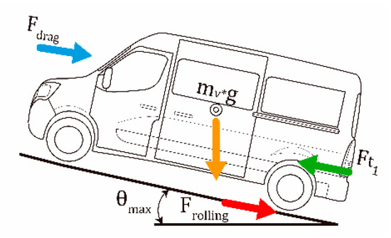
Figure 1.
Forces distribution along longitudinal axis of the vehicle for case 1.
For case 1, the principle of forces is determined using Equation (1). Acceleration (ẍ) is determined by the need to go from zero to the chosen top speed. Poor acceleration makes traffic uncomfortable on the road and a high acceleration demands a powerful engine/motor.
where the traction climbing force is Fclimb, the aerodynamic force is Fdrag and the force due to rolling resistance is Frolling.
For case 2, where the vehicle travels at the max speed,
Where Fdrag2 is the aerodynamic force and Frolling2 is the force due to rolling resistance for case 2.
The power required by the engine/motor is determined using Equation (3), Ft is the greatest force for both cases Ft1 and Ft2, and ẋ is the linear speed of the vehicle corresponding to this force.
The selected engine/motor power is determined by Po plus the sum of the additional power required by the vehicle’s accessories. From this selection, it is possible to obtain maximum torque Tomt at its respective speed ωmt, and torque Topow at maximum power at a specified speed.
2.3. Speed Ratio of CVT and Gearbox
Once the engine/motor is selected, it is time to calculate the overall speed ratio of the system. A powertrain for EV usually consists of a gearbox, differential reducer, and a CVT [11,27] or a transaxle with a CVT. The first speed ratio is determined for case 2 when Rcvt_min has a minimum value of 1:1. For this case, the vehicle is at maximum linear speed and the engine/motor will be working at the maximum power zone. Towh is the wheel torque and η is the efficiency. It is possible to have a speed ratio of less than one, yet it is not efficient to increase angular speed to then reduce it again within the powertrain.
Equation (9) is used to determine the maximum fixed reduction system ratio (gearbox and/or differential reducer). However, its design is not discussed further in this article. For case 1, the vehicle uses the energy to overcome mainly its inertia on climbs. Using Rgear and Equations (6) and (7) the maximum CVT speed ratio Rcvt_max can be determined.
2.4. Rubber V-Belt Selection
CVT belts are commercially available, and feature both metric and imperial systems. The belt tension capacity (FTmax) is a function of the section dimensions. For a wider belt there is a tendency to have a greater number of reinforcement members; and at higher heights, it tends to have a thicker friction surface and a higher minimum diameter. The belt reinforcement’s quality indicates the specific tension value in (N/mm2) it can withstand. The maximum tension supported by the belt is the product of the sectional area multiplied by its maximum specific stress. Also, the belt must resist tensile forces such as working tension (FTwork), centrifugal force (FTce) tension which is a function of the radius, the linear density of the belt, the angular speed (rpm), and bending tension (FTdo) when passing through the pulleys. This latter tension is a function of the belt thickness and the radius pulleys (Figure 2).
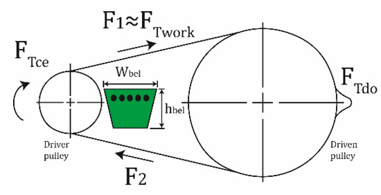
Figure 2.
Working tensions in the rubber V-belt.
The sum of the working tension, the centrifugal force tension, and the bending tension must not be greater than the maximum tension of the belt (Equation (9)). Therefore, an iterative process based on commercial references is presented to determine the minimum driver pulley diameter and the belt section selection (Figure 3). The minimum pulley diameter depends on CVT belts specifications, such as belt thickness, topology, whether it has teeth on the inside and outside face which decrease the bending stress, and the side section area of the belt. The process begins by selecting an initial belt section from where to obtain transversal area value (Abelt); section dimensions such as width (Wbel); thickness (hbel); belt angle (φbel); maximum tensile stress; and belt density (ρbel). Then, these tensions and the minimum operational diameter are determined. The minimum driver pulley diameter (ϕ1_min) is determined using Equation (8); this equation was developed by iterating the minimum diameter until the bending stress is significant. The diameter can also be checked in norms and standards [34]. It is verified that for the entire range of motor angular speeds (rpm) the sum of tensions is not greater than the tension that the belt withstand (Equation (9)). Finally, it is validated that the recommended lateral pressure is not exceeded either.
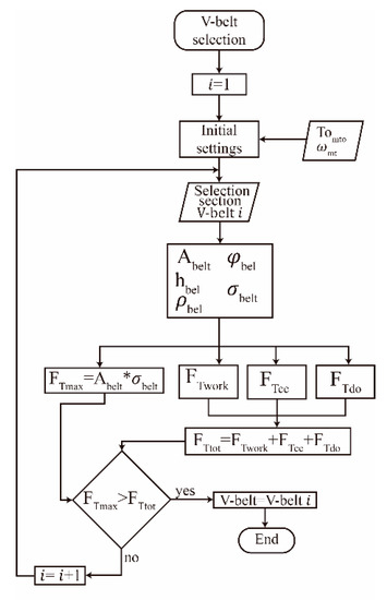
Figure 3.
Belt selection flowchart.
The maximum stress that the belt can withstand is a function of the material’s properties. In Equation (10) this stress is calculated, where σbelt is the maximum tensile stress.
The working tension is given by Equation (11), where (ϕ1_min) is the minimum driver pulley diameter.
Assuming that the non-tensioned side of the belt is not significant when compared to the tensioned side, due to the high friction coefficient μ between the pulley-belt and the belt angle (ϕbel), the approximation in Equation (12) is proposed. By calculating the working force it is possible to solve the minimum pulley diameter (ϕ1_min) using Equation (11).
The tension produced by the centrifugal force is mainly given to the linear speed of the belt (VLbelt).
The linear speed belt can be determined from the following expression, where ωmt is the angular speed at maximum engine/motor torque.
The belt density can be determined using Equation (16), where ρlbel is the belt’s lineal density from manufacturers.
A bending stress is produced when the belt passes through the pulleys. This stress is a function of the relationship between the belt thickness and the belt diameter. εbb is the equivalent bending stress considering the location of the reinforcements in the transversal section and the belt teeth geometry.
2.5. Pulley Center Distance and Belt Length
The distance between centers of CVT pulleys (C) for vehicles should be kept to a minimum given the space in which they are located [33]. The limitation is given by the contact angle τcc between the belt and the smallest pulley, knowing that τcc ≥ 160° avoids the torque losses. An approach to determine C considering this constraint is to analyze the right triangle (Figure 4) which is formed between the two pulleys at the max speed ratio using Equation (18).
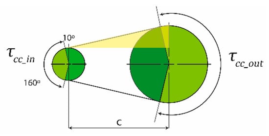
Figure 4.
Distance between centers and τcc.
By accepting this approximation, it can be established that the length of the rubber V-belt is then:
where ϕ2_max is the maximum driven diameter and it is determined with the expression (ϕ1_min Rcvt_max). The values for the driver and driven pulley’s contact angles are τcc_in and τcc_out respectively. The exact angle of contact between the belt and driver pulley is,
The exact angle of contact between the belt and driven pulley is,
2.6. Complementary Diameters
Dimensions for the driver and driven pulleys can be determined by knowing the minimum and maximum speed ratios of the CVT system (Rcvt_min and Rcvt_max) (Table 1).

Table 1.
Continuously variable transmission (CVT) pulley diameters.
2.7. Lateral Displacement, Tensile and Clamping Forces
The belt angle φbel and the minimum and maximum radius of the pulleys determine the lateral displacement σLat (Figure 5).
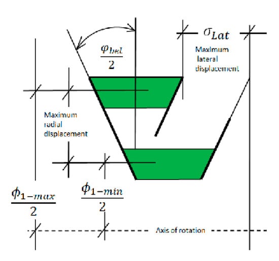
Figure 5.
Lateral displacement scheme.
Trigonometric relationships are constructed with the geometry of the pulley and the belt (Figure 6), which relate the parameters to the radial force (Frad), the normal force (FNor), the clamping force (Fcl) and the tangential tension to the belt centerline which is equivalent to the friction force (Ffric) between the belt and the pulley without considering slip [35]. The following equations describe these forces as a function of the tensions F1 and F2, F1 is calculated considering Equation (12).
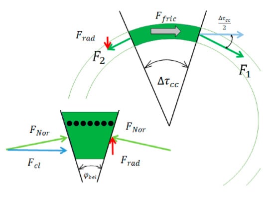
Figure 6.
Rubber V-belt system forces.
2.8. Misalignment of Pulleys by Diameter Change
Lateral displacement is not the same when the pulleys change diameter. This causes a misalignment in the system, which is calculated using Equation (27) for each pulley, in order to verify if the maximum permissible value is exceeded. Two cases are analyzed, first when the driver pulley is in its minimum diameter and the driven pulley is maximum in diameter, and the second case when the inverse occurs. This is done to consider the minimum and maximum possible ratios.
To prevent belt crossing, different pulley angles are used φpull_1 and φpull_2. One is larger than the belt angle φbel and the other one smaller, without exceeding the degrees that affect the contact between the belt and the pulley. The admitted angle variation can be between two and three degrees.
2.9. Force Balance
The difference in clamping forces in the driver and driven pulleys for CVT systems leads to a change in the ratio Rcvt. When the lateral force of the driver pulley exceeds the driven one, a lateral closing displacement in the driver pulley occurs and the belt occupies a greater radius. Given that the length of the belt is fixed, the driven pulley will open where the belt movers to a lower radius. This change in radius modifies the ratio between them, increasing the speed of the driven pulley.
In this case, there is a set of centrifugal elements to develop these forces in the driver pulley. These involve a ramp which reorients part of the radial force (Fcen) in an axial or lateral direction to the pulley. For the driven pulley, this force is derived from a spring. The increase or decrease in this force is carried out by compressing the spring with a cam. To transmit more torque the cam compresses the spring which is actuated by the torque on the output shaft.
These lateral forces have an additional function, they produce a lateral compression on the belt called clamping force (Fcl), which prevents the belt from slipping and losing efficiency. Figure 7 presents four possibilities for this balance of forces, which determines the dynamics of the mechanism. The numbers correspond to the positions of the torque and angular speed graph in Figure 8.
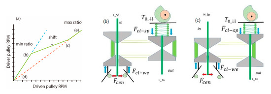
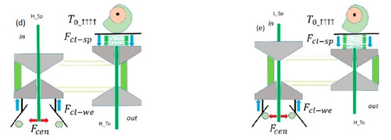
Figure 7.
(a) Possible operational situations: low speed, high torque (b); high speed, high torque (c); low speed, low torque (d); high speed, low torque (e).
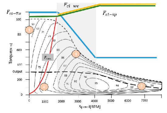
Figure 8.
The clamping force (blue), the centrifugal force (red), the centrifugal force’s lateral component (yellow) and the spring force (green) are drawn over the torque and angular speed motor.
Before calculating the parameters of the centrifugal actuator, certain data must be defined, which then results in a graph as presented in Figure 8. A blue curve is drawn on the motor torque graph, which proportionally corresponds to the lateral force required to transmit the torque without slippage. Additionally, the centrifugal force is shown in red; the desired component of the centrifugal force in the axial or lateral direction in orange; and the required lateral force on the driven pulley spring in green. Finally, in Figure 8 the ratio change zone is highlighted in a grey section. The designer chooses two engine speeds: the rpm ωCVT_ini where the CVT should start changing ratio, usually close to the maximum torque, and a second speed ωCVT_end where the speed ratio change should end, usually near maximum engine efficiency.
2.10. Driver Pulley Actuators
The driver pulley for CVT systems has centrifugal actuators in conjunction with a spring that generates the clamping force required to perform the transmission ratio change Rcvt [22]. As shown in Figure 9, there are two types of CVTs, each with advantages and disadvantages. The first type are weight and ramp systems and the second a flyweight cam system.
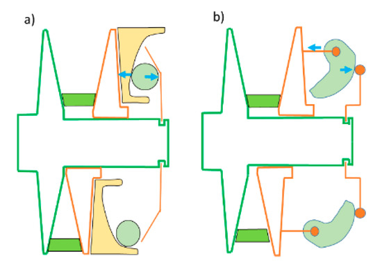
Figure 9.
Centrifugal actuation system: (a) ramps and roller weights, (b) flyweight cam.
2.10.1. Ramp and Weight System Design
The method for achieving this centrifugal force, which is nevertheless changing and has a component in the axial direction, consists of placing three weights (mwe) on the driver pulley with the possibility of them moving radially. When the pulley is rotated, the weights will experience a centrifugal force, then the weights will be displaced in a ramp that has a variable angle such that the axial component varies, as shown in Figure 10.
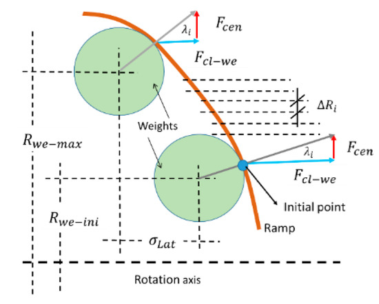
Figure 10.
Diagram of axial force (Fcl_we) derived from the centrifugal force due to the ramp.
Knowing the maximum and minimum values in the change zone (Figure 8) for angular speed, displacements, forces, and speed ratio, ranges are established and divided into nwe range differentials. In order to obtain the result, each weight’s radial displacement differential is associated with the required lateral force, a centrifugal force, an angular speed, a speed ratio, and the ramp angle is to be calculated. The location of the starting point for the first ramp differential is an input parameter in the iterative method. For each iteration, the previous differential points are connected to the beginning of the next one in order to generate continuity. The result is the ramp or profile of the actuator as shown in the example in Section 4.
For the ramp’s design, an iterative calculation process is initiated with i = 1 to i = nwe using the Equations (28)–(38) for each iteration, and considering the following:
- The speed range in which the CVT changes from ratio Rcvt_max to Rcvt_min and (grey zone in Figure 8) to the maximum engine/motor speed.
- The centrifugal force Fcen_i at each speed (Figure 8, red line).
- The clamping force weights value (Fcl_we_i) required at each speed (Figure 8, orange line). Fcl_we_ini and Fcl_we_end are the initial and final force range.
- The radial displacement Rwe_i of the weights at each speed. Rwe_min and Rwe_max are the maximum and minimum radius displacement.
The ramp’s orientation angle (λi) is calculated for each speed ωi of the driver pulley, where i is the iteration number.
where vlωe is the tangential speed of weights and MAωe the weights mechanical advantage.
2.10.2. Centrifugal Flyweight Cam Design
Flyweight cams which have a profile according to lateral force requirements are yet another mechanism found in the field of centrifugal actuators for driver pulleys. The operational principle is shown in Figure 9. The cam pivots on its rotation axis at one end. The center of gravity is located next to the rotation axis and separated from the pulley rotation axis. Then the flyweight is exposed to a centrifugal force that tends to make it turn and displace. The cylindrical follower prevents the flyweight from turning freely. The flyweight and follower pivot shaft are attached to the pulley frame and the moving face, respectively (Figure 9). When the flyweight tries to turn it produces a force that pushes the follower. This force experiments with a reaction that pushes the moving plate of the driver pulley until it moves and, thus, closes the space that the belt occupies; then the rubber V-belt occupies a greater radius, which produces the speed ratio change.
Similar to the design of the ramps and weights, the cam profile is defined by the clamping force and the centrifugal force that occurs at the point of contact with the follower. Using the lever law, the equivalent centrifugal force Fcc and the lateral component of this force Fcl (Figure 11, blue arrow) are located at the point of contact between the cam and the follower. The method begins by drawing an auxiliary line through the pivot point of the flyweight and the center of gravity of the cam. An auxiliary coordinate system () is created on this line (Figure 12).
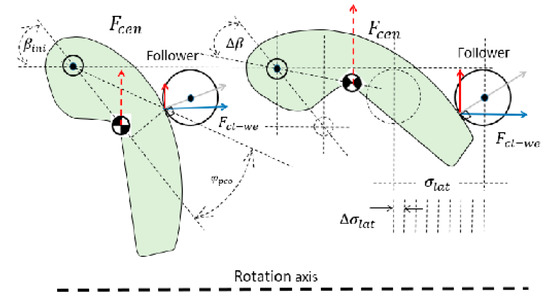
Figure 11.
Lateral force principle by flyweight cam.
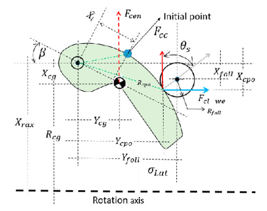
Figure 12.
Parameter and variable naming in flyweight cam.
The following step is to select a starting point (, Ŷini) in the flyweight profile. This point corresponds to the initial angle βini of the flyweight and the initial distance of the follower σfoll_ini. Figure 8 shows the ratio change sector in the grey area. Here, initial and final speeds between which the ratio change occurs is declared. Immediately associated with each speed is the change in lateral displacement for the moving face of the driver pulley. As in the design case of centrifugal weight and ramp actuator, ranges are also declared and divided into nwe range differentials.
The lateral displacement of the follower center σlat is declared as an independent variable and the centrifugal force is calculated using the center of gravity location data, the flyweight angle βi-1, and the initial contact point of the flyweight and the follower (Xcpo, Ycpo). The differential’s inclination θs is calculated in the flyweight profile ramp using the centrifugal force (Fcen) and the required clamping force (Fcl). If the center of gravity is located at a different site, the unusable weight should be relocated to different places where it is ensured that the center of gravity is relocated to the initially chosen point (Xcg, Ycg). This implies that the mass (mlen) is constant.
The starting point of the ramp profile differential is linked to the endpoint of the previous iteration. In each iteration the previous differential is connected to the new one in such way that the end of the first one will coincide with the starting point of the second one. As shown in Figure 13, within the procedure there is a trigonometric correlation between the flyweight cam angle β, the contact point angle φcpo, and the tangent angle at the contact point θ. With these three angles, the initial or acquired parameters, and the previous iteration data, the system is solved. The method used here is implicit, and several iterations are made to optimize the result.
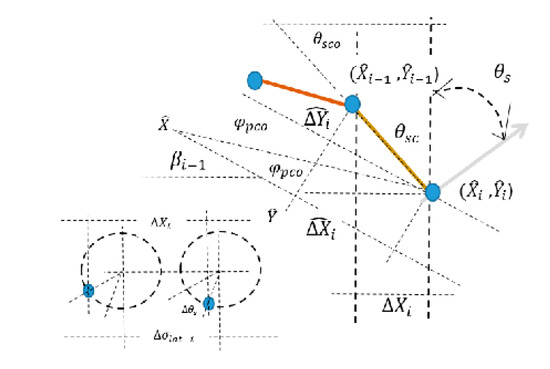
Figure 13.
Trigonometric relationships of the mechanism.
With the clamping force and the Equations (39)–(50), an iterative calculation process is started with i = 1 to i = nwe. The sub-index (i) and (i−1) represents the actual and last iteration, respectively.
where ωm_max is the maximum angular motor speed; Rcg is the radius from the rotation axis to the flyweight center of gravity; Xrax is the distance from rotation axis to flyweight fixed point; and Rcpo is the radius from rotation axis to the contact point between the flyweight and the follower.
2.11. Driven Pulley Spring Design
The torque sensor cam is not a disk cam as shown for didactic purposes in Figure 7, instead it is a cylindrical cam. The driven pulley spring must be pre-compressed to a given value Xp_sp and when the CVT is on its high ratio Rcvt_max it exerts a force equal to the amount required by the clamping force Fcl (Equation (52)). It also has to be able to be compressed to a length equal to or greater than the lateral displacement of the pulley σLat. The spring constant Ksp depends of the turn number (nsp); spring diameter (ϕsp); shear stress (G); wire spring diameter (dw); and the spring clamping force (Fcl_sp).
2.12. Torque Sensing Cam Design
The spring is required to provide enough lateral force so that the belt does not slip during the start of high torque. This requirement calls for a spring that does not decrease in force as the motor /engine speed increases, therefore, decreasing the amount of available torque, as shown in Figure 14. The effect of having lateral force that is higher than required (Figure 14, blue line) results in greater friction losses between the belt and the pulleys and, therefore, in a drop in system efficiency. To solve this problem, engineers added a cam on the driven pulley located on the output shaft. This cam responds to shaft torque, compresses at high torque values, and decompresses at low torque values. The result is equivalent to having multiple springs, shown as a green dotted line in Figure 14. The result is that when the torque is increased, both axes acquire an offset angle εsp_i and an axial displacement σaxi_i this is due to the ramp as seen in Figure 15.
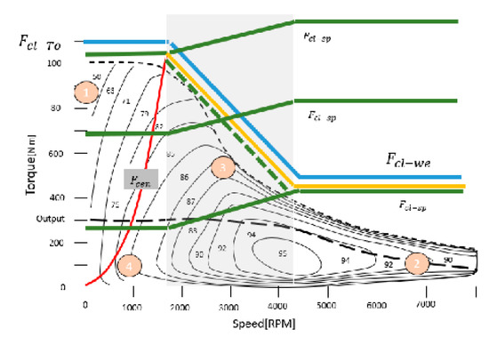
Figure 14.
Force graph including the speed ratio change and the sensing torque cam effect.
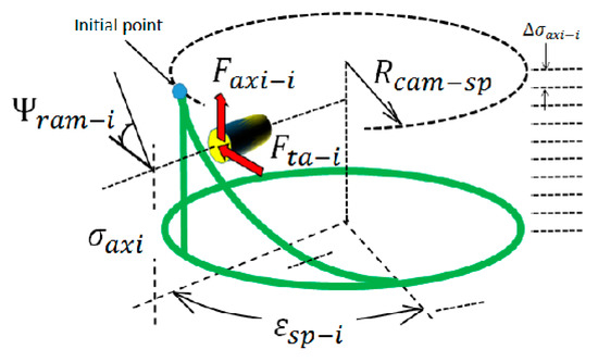
Figure 15.
Torque sensing cam diagram.
The grey area of Figure 14 shows the ratio change zone. From there, the maximum and minimum values of torques; displacements; forces; reduction ratio; and angular speed are obtained and thus the ranges are established and divided into differentials nwe. Each lateral displacement differential for the cam follower is associated with its required lateral force, a torque on the driver and driven pulley, an angular speed, and a speed ratio, then the cam profile angle is calculated.
The location of the starting point for the first ramp differential is an input parameter in the iterative method. For each iteration to generate continuity the points of the previous differential are connected to the starting points of the next one. The result is the actuator ramp as shown in the example in Section 4. The design of the torque sensor cam (Equations (53)–(63)) is divided into nwe parts that consider the following:
- The torque range to be affected (Ti). Tini is the initial torque and Tmin the minimum torque.
- The spring force range (Fsp_i) according to the torque. Fsp_ini is the initial spring force.
- The axial displacement of the cam ∆σaxi_i.
3. Methodology
To compare and validate this proposed method, three types of test are performed: (a) a measurement and characterization of all the elements and components of a commercial CVT is elaborated. The values are used as parameters in the design using the equations presented. The capacity in torque, speed ratio, and others are compared with the manufacturers’ specifications. This testing is carried out on the test bench. (b) Using this method, a design for a powertrain composed of a rubber V-belt CVT and a differential reducer is presented. (c) The behavior of the designed CVT operating in an electric vehicle is simulated running a stringent route.
To validate the proposed numerical design method, a computer simulation tool is developed which sequentially addresses the different steps presented. This tool solves the iterations and equations using Runge–Kutta’s method. For the selection of the commercial elements, a database is created taking the greatest amount of specifications that can be obtained, and then introduced into the computer simulation tool. With this application, a programming object that uses the results of the design is developed, and it performs as such in a complete vehicle model that includes other remaining objects.
For the method development, some aspects were found in the literature and others had to be validated. The test bench is a device in which data from the road and the vehicle as weight of the vehicle along the road, number of random or fixed stops, and the desired cruise speed are introduced. The vehicle or powertrain is tested in the device to obtain information about torques, speeds, currents, and energy consumption. Figure 16 shows the elements that make up the vehicle and the dynamometer that allows for the acquisition of real-time data from the powertrain. Its characteristics and components are 1. Commercial CVT: Polaris, USA, sportsman 500 primary drive clutch 1996–2011; Team, USA, tied driven secondary clutch 421896, Gates, USA, 19G4006E G-force CVT belt; 2. Galoce, China, GTS100 torque sensor (150 Nm); 3. Electric motor and controller HPEVS, USA, AC20 + Curtis instruments, USA, 1238E-7621; 4. Galoce, China, Torque sensor GTS-100 torque sensor (1000 Nm); 5. Flowfit, UK, Gearbox 40-97001-3.8 gear ratio 3.8; 6. DANA SPICER, USA, 520290T-3X differential D-max gear ratio 4.3; 7. 2 Brakes load capacity 1400 Nm; 8. Wheels 255/70R17.5. These are part of a kit with various motors, gearboxes and some own made CVTs. Due to the maximum size of vehicles available, the variation of rubber V-belt CVTs is given only from a width of 32 mm until the industrial or agricultural belts with a width of 100 mm.
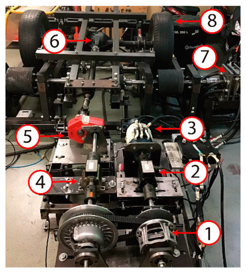
Figure 16.
Testing bench: active dynamometer.
Using this test bench, a powertrain operated simulating different torques and angular speed. Data obtained and the inferences from these test were used in order to make considerations, which were converted into algorithms or equations providing robustness to the design method and the computer tool. The design process of the gear systems was not evaluated in this analysis. The following parameters can be measured on the test bench torque and speed at the input and output of the CVT shafts: angular and linear speed at the rollers where the wheels are located; brake pressure; brake temperature; motor temperature; and voltage and current of the energy system. This data are collected by a Delta, Taiwan, PLC (DVP28SV211T) using digital and analog signals and then analyzed in real-time in LabVIEW SP1 2019. The test bench and the powertrain can be configured with the components list in Table 2.
Table 2.
Test bench and powertrain components.
The route chosen to test the vehicle’s CVT (in the simulation software) has a distance of 15.704 km; a range of slopes from 4° to 16°; a maximum speed of 80 km/h and an average speed of approximately 27.8 km/h, and conditions of active and passive load of 5500 N without variation over the entire route. Some of this data were collected from a previous study for a public transport vehicle that circulates every day on this same route. The concurrent vehicles on this route are powered by ICE, have a 5 shift-speed gearbox, and a power between 100–130 KW.
4. Example Analysis and Discussion
A powertrain design composed of a CVT and a fixed gear transmission for a common city vehicle transmission is presented. Typically mountainous towns have small buses (22–28 passengers), delivery cars, and fire and police trucks, among others, with cargo capacities of approximately 3000 or 4000 kg. These vehicles do not exceed speeds of 80 km/h in their operation and their average operating speed is 30 km/h. Chosen routes have between 4 and 15 km of maximum travel, with inclination angles between 4° and 16°. One of the reasons for these vehicles to be small is that they travel on city slopes and these roads are usually narrow and with low curvature radius. The characteristics used for the analysis of the vehicle powertrain are: gross vehicle mass of 5500 kg, aerodynamic coefficient of 0.45, front area 3.5 m2, air density 0.98 kg/m3, the rolling coefficient is 0.03, wheel diameter approximately 0.75 m (R17.5). The aim is for the loaded vehicle to achieve maximum speed on slopes within 5 s. This results in a climb acceleration of 1.7 m/s2 and a maximum speed of 30 km/h on slopes and 80 km/h on flat routes.
Using equations (1)–(3) it is determined that the peak power for the vehicle is 130 KW on a 16° slope and 45 KW continuous power on flat routes. Recent recurring problems in vehicle design are the reduction of polluting emissions, increasing overall efficiency, and improving energy performance. A solution to this problem is the use of EV, therefore, this type of vehicle is the one chosen. New electric motors tend to operate at high rpm (>6000) to decrease the weight per power unit. However, for these angular speeds the belts would exceed the allowable tangential speed (approximately 30 m/s) and a fatigue of the V-belt could occur, as a result of the available tensile capacity being reduced by the effect of the centrifugal force. Therefore, a motor with a maximum rpm in the order of 4000 rpm should be selected with the requirements of having a continuous torque value of 500 Nm at 1500 rpm and a peak value of 840 Nm. After analyzing the possibilities in the market, the motor described in Figure 17 was chosen.
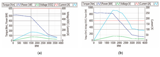
Figure 17.
Electric motor curves: (a) continuous graph; (b) peak graph.
The ratio of the fixed transmission system is obtained using Equations (4) and (5), the Rgear has a value of 6.2. Configurations may vary, for instance, it is possible to have a single gearbox and a differential or a transaxle. According to Equations (6) and (7) the maximum ratio of the CVT is RCVT_max = 1.94. Finally, the maximum speed ratio of the system is 12. In this case, the system is composed of an electric motor, a CVT, and a differential as show in Figure 18.
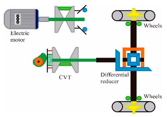
Figure 18.
Electric powertrain.
The belt section is determined using the iterative process in Figure 3, for which the commercial belt section that most closely approximates the parameters is the W100 reference. It has a width Wbel of 100 mm, a thickness hbel of 32 mm, a belt angle φbel of 30°, and a cross-sectional area of 3050 mm2. The maximum tension present in the belt is 11,858 N determined by the sum of the three tensions. Assuming that the belt tensile strength (σbelt) is 4 N/mm2, the minimum cross-sectional area of the section is obtained using the Equation (10) of 2965 mm2, afterwards the aforementioned belt is selected as it is the closest to this value.
The tensions that interact on the belt are the working tension, the tension due to the centrifugal force, and the bending tension. Using Equation (11) it is determined that the value of the working tension is 8840 N with a starting torque of 840 Nm and a diameter ϕ1_min of 193 mm. A more precise value of this tension is obtained using Equation (12) with a result of 8750 Nm, considering a friction coefficient μ between the belt and the pulley of 0.5. The tension due to the centrifugal force adds a value of 995 N (Equation (14)) with a belt density of 1.32 kg/dm3 (Equation (16)). Belts with deep and short teeth have low bending stress [36], considering a bending stress of 15 N/mm2 the bending tension is 2013 N (Equation (17)).
The minimum diameter ϕ1_min for a V-belt with a thickness of 32 mm is 193 mm (Equation (8)). With the value of the maximum CVT speed ratio Rcvt_max, it is determined that the maximum driven pulley diameter is 384 mm. The pulleys diameter to develop a minimum ratio of 1:1 is 278 mm. The minimum pulley center distance C is 300 mm (Equation (18)) using the τcc_in ≥ 160° approximation. However, the pulleys are almost rubbing against each other, and to correct this the contact angle is increased to 166° obtaining a value of C of 400 mm which allows for an increase in the tensile capacity. Finally, the belt’s length is 1674 mm.
The lateral belt displacement in the driver pulley is 23.57 mm and 29.95 mm in the driven pulley (Equation (22)), and this causes the belt to be crossed by 0.69° (Equation (27)). To enhance alignment, the driven pulley angle is reduced to 28°, ergo its lateral displacement is reduced to 26.42 mm and the misalignment to 0.4°, which reduces the crossing belt by 57.97%. This modification generates a small distortion between the lateral forces on both pulleys when the belt passes from one to the other. The maximum normal lateral pressure reaches 9 kg/cm2. The lateral force on the belt is 7600 N on average (Equations (13) and (23)) or 8600 N as a result of the integral (Equation (26)) and a 160° contact angle. The lateral force to prevent the belt slip is in the range from 8540–1415 Nm (Figure 19b).
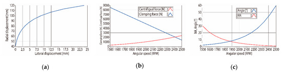
Figure 19.
(a) The profile of the ramp on which the weight moves radially; (b) the available centrifugal force and the required clamping force as a function of the rpm; (c) mechanical advantage (MA) or relationship between the forces and the ramp angle to develop the clamping force.
Figure 17 shows the CVT ratio change zone, starting at the point where the torque starts decreasing (1500 rpm) and ending at the sector where the motor’s efficiency is the highest (2500 rpm). The torque range is 840 to 200 Nm. In this case, for the design of the centrifugal actuator, we have a ramp and weight system. Using the Equations (28)–(38) we can find the form of the ramp, the values and relationships between the centrifugal and clamping force, and the angle and mechanical advantage as a rotational speed function. The data obtained are initial ramp radius 40 mm and a final ramp radius of 120 mm, lateral displacement of 23.57 mm, and the mass of the weights is found by iterations. If the weight grows the lateral displacement grows, and vice versa. For the required displacement, the total weight is 288 g for the three weights.
For low rpm the centrifugal force is low (285 N) but the required clamping force is high (8540 N) so the mechanical advantage must be high (30:1). This is achieved by using a near radial angle (1.9°) on the ramp. The opposite situation occurs at high speed, high centrifugal force (2096 N) and low clamping force (1415 N). In this case, the angle will turn to the right with a higher value regarding the radial axis (46.2°).
For the driven pulley, a spring and a cylindrical cam are designed to regulate the clamping force according to the torque and the change in diameter for the pulley. The driven pulley spring is compressed at maximum torque applying a maximum lateral clamping force. As the torque changes the spring expands and at the same time, it responds to displacement due to the speed ratio change that compresses it by a maximum of 24 mm. With a minimum spring diameter of 70 mm, and using Equations (51) and (52), the spring constant is determined with a value of 140 N/mm. The displacement of the spring is 60 mm and the free length is 175 mm, the diameter of the spring wire is 14 mm made of piano wire rope that provides a torsional stress of 727 N/mm2 at maximum compression, and a 10 mm pre-compression for minimum clamping force. The cam that compresses the spring is designed with Equations (52)–(62). The torque range when the CVT changes from maximum to minimum speed ratio is 1620–400 Nm. The diameter of the cam is designated a value of 150 mm.
In this case, the graphs should be read backwards from 50–0 mm axial displacement (Figure 20), which is equivalent to the initial condition in the driver pulley. An angle of 69.35° is used to balance the maximum torque (1620 Nm) which is equivalent to 21,600 N of tangential force with the clamping force (8540 N) and the mechanical advantage (2.65).
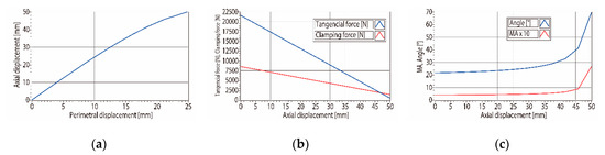
Figure 20.
(a) Cylindrical cam profile, (b) tangential and axial force as a function of axial displacement, (c) relationship between forces and profile angle as a function of axial displacement.
Finally, this powertrain is simulated in a vehicle with the above characteristics. The route has a total distance of 15.704 km, inclinations vary between 4° and 16°, a real travel time of 33.8 min, and the average speed of the route is 27.80 km/h. It is necessary to establish that these data were collected in a previous exploration of several routes in a city with mountainous topographic conditions and bus weights corresponding to mass public transport vehicles. As a result of this study a dynamic simulation software for vehicles was developed, and used for elaborating the simulations for this.
The linear vehicle speeds distribution along the route can be observed in Figure 21. In this case, the powertrain design is based on a vehicle that does not operate high speeds, and which operates between 20 and 40 km/h for half of its travel time. This type of transport is presented in cities that have services from feeder buses to other vehicles of greater affluence.
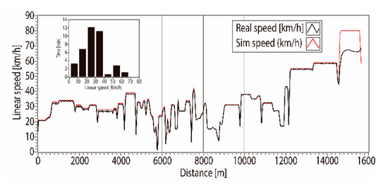
Figure 21.
Lineal vehicle speed.
The powertrain is composed of a CVT with the speed ratio characteristics present in Figure 22, the CVT operates on an average ratio of 1.597.
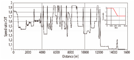
Figure 22.
CVT speed ratio during the route.
The CVT system configuration allows for the currents achieved by the electric motor to remain below the values of its continuous curve, and the high current peaks occur during short distances and short time (Figure 23).
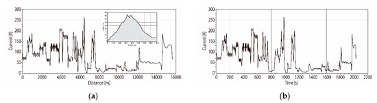
Figure 23.
(a) Motor current on the travel road and road topography, (b) Motor current on time.
The total route has an energy consumption of 22.3919 KWh. In the simulation, the regenerative brake was not included in the system. We assume that if it is considered, performance will improved.
5. Conclusions
A method of sequential equations is presented to enable the implementation of a computer application and to perform the analysis and assignment of all dimensional and operational parameters for a rubber V-belt CVT design. The increasing use of vehicles that only travel specific routes and have low dynamic demands is addressed by the method by providing an advantage for the design of vehicles that operate at their highest possible efficiency. The reason is that the sequential design process based on user needs, in terms of road, vehicle characteristics, and desired performance integrates the system in a way that each particular need can be analyzed from all aspects that influence the results.
A CVT system design becomes a complex problem due to the number of interactions and relationships between forces in the pulleys. Due to the strong interrelationship between parameters and variable values, implicit equations are present in the design that exclude analytical methods as practical tools. Using numerical methods and equations, the proposed method provides simplified equations and data for developing a design and solution for the complex interactions in the CVT design.
The desired vehicle behavior generates variations in actuators’ geometry. However, the numerical method allows for a fast convergence in the approximation of the result in the design of either type of pulley actuator. Compared to an ICE, which at low rpm has low torque, an electric motor provides maximum torque and generates a minimum centrifugal force in the CVT driver pulley. This difference requires the driver ramp to have a different profile.
Commercial rubber V-belts have a wide range of applications in the transport industry, especially in EV. Using the method for each type of standard rubber V-belts, a diverse range of applications can be addressed in vehicles from three-wheelers to medium cargo vehicles as presented in the results. The advantage of using a CVT in a vehicle is the reduction in the size of the motor and its characteristics. Compared to a fixed transmission, the vehicle would have lower speeds on plane routes or would need a larger motor to be able to start on inclined routes. Furthermore, the system would also operate outside the maximum efficiency range.
Author Contributions
Conceptualization, I.A.; methodology, S.M.A.; software, I.A. and S.M.A.; validation, I.A. and S.M.A.; formal analysis, I.A. and S.M.A.; investigation, I.A. and S.M.A.; writing—original draft preparation, S.M.A.; writing—review and editing, I.A. and S.M.A.; supervision, I.A.; project administration, I.A. All authors have read and agreed to the published version of the manuscript.
Funding
This research was funded by Departamento Administrativo de Ciencia, Tecnología e Innovación (COLCIENCIAS) (Grant No 033-2018); and EAFIT University.
Conflicts of Interest
The authors declare no conflict of interest.
References
- Yildiz, A.; Piccininni, A.; Bottiglione, F.; Carbone, G. Modeling Chain Continuously Variable Transmission for Direct Implementation in Transmission Control. Mech. Mach. Theory 2016, 105, 428–440. [Google Scholar] [CrossRef]
- Srivastava, N.; Haque, I. A Review on Belt and Chain Continuously Variable Transmissions (CVT): Dynamics and Control. Mech. Mach. Theory 2009, 44, 19–41. [Google Scholar] [CrossRef]
- Cholis, N.; Ariyono, S.; Priyandoko, G. Design of Single Acting Pulley Actuator (SAPA) Continuously Variable Transmission (CVT). Energy Procedia 2015, 68, 389–397. [Google Scholar] [CrossRef]
- Kim, K.; Kim, H. AXIAL FORCES OF A V-BELT CVT PART I: THEORETICAL ANALYSIS. KSME J. 1989, 3, 56–61. [Google Scholar] [CrossRef]
- Ruan, J.; Walker, P.; Zhang, N. Comparison of Power Consumption Efficiency of CVT and Multi-Speed Transmissions for Electric Vehicle. Int. J. Automot. Eng. 2018, 9, 268–275. [Google Scholar] [CrossRef]
- Greene, D.L.; Baker, H.H., Jr.; Plotkin, S.E. Reducing Greenhouse Gas Emissions from US Transportation. Prep. Pew Cent. Glob. Clim. Chang. 2010. [Google Scholar] [CrossRef]
- Brace, C.; Deacon, M.; Vaughan, N.D.; Horrocks, R.W.; Burrows, C.R. The Compromise in Reducing Exhaust Emissions and Fuel Consumption from a Diesel CVT Powertrain over Typical Usage Cycles. In Proceedings of the CVT’99, Eindhoven, The Netherlands, 16–17 September 1999; Volume 99, pp. 27–33. [Google Scholar]
- Brace, C.; Deacon, M.; Vaughan, N.D.; Burrows, C.R.; Horrocks, R.W. Integrated Passenger Car Diesel CVT Powertrain Control for Economy and Low Emissions. Management 1997, 25, 26. [Google Scholar]
- Zhu, C.; Liu, H.; Tian, J.; Xiao, Q.; Du, X. Experimental investigation on the efficiency of the pulley-drive cvt. Int. J. Automot. Technol. 2010, 11, 257–261. [Google Scholar] [CrossRef]
- Hofman, T.; Janssen, N.H.J. Integrated Design Optimization of the Transmission System and Vehicle Control for Electric Vehicles. IFAC-PapersOnLine 2017, 50, 10072–10077. [Google Scholar] [CrossRef]
- Bottiglione, F.; De Pinto, S.; Mantriota, G.; Sorniotti, A. Energy Consumption of a Battery Electric Vehicle with Infinitely Variable Transmission. Energies 2014, 7, 8317–8337. [Google Scholar] [CrossRef]
- Hofman, T.; Dai, C.H. Energy Efficiency Analysis and Comparison of Transmission Technologies for an Electric Vehicle. In Proceedings of the IEEE Vehicle Power and Propulsion Conference (VPPC 2010), Lille, France, 1–3 September 2010; pp. 1–6. [Google Scholar] [CrossRef]
- Kluger, M.A.; Long, D.M. An Overview of Current Automatic, Manual and Continuously Variable Transmission Efficiencies and Their Projected Future Improvements. SAE Trans. 1999. [Google Scholar] [CrossRef]
- Kobayashi, D.; Mabuchi, Y.; Katoh, Y. A Study on the Torque Capacity of a Metal Pushing V-Belt for CVTs. In Proceedings of the International Congress and Exposition, Detroit, Michigan, 23–26 February 1998. [Google Scholar] [CrossRef]
- Ferrando, F.; Martin, F.; Rjba, C. Axial Force Test and Modelling of the V-Belt Continuously Variable Transmission for Mopeds. J. Mech. Des. Trans. ASME 1996, 118, 266–273. [Google Scholar] [CrossRef]
- Mussaeus, M.A.; Serrarens, A.F.A.; Veldpaus, F.E. CVT Ratio Optimization for Minimal System Losses in Passenger Cars *. IFAC Proc. Vol. 1998, 31, 125–130. [Google Scholar] [CrossRef]
- Grzegozek, W.; Dobaj, K.; Kot, A. Experimental Verification and Comparison of the Rubber V- Belt Continuously Variable Transmission Models. IOP Conf. Ser. Mater. Sci. Eng. 2016, 148. [Google Scholar] [CrossRef]
- Asayama, H.; Kawai, J.; Tonohata, A.; Adachi, M. Mechanism of Metal Pushing Belt. JSAE Rev. 1995, 16, 137–143. [Google Scholar] [CrossRef]
- Kim, H.; Lee, J. Analysis of belt behavior and slip characteristics for a metal v-belt cvt. Mech. Mach. Theory 1994, 29, 865–876. [Google Scholar] [CrossRef]
- Lee, H.; Kim, H. Analysis of Primary and Secondary Thrusts for a Metal Belt CVT Part 1: New Formula for Speed Ratio-Torque-Thrust Relationship Considering Band Tension and Block Compression. SAE Technol. Pap. 2000, 2000. [Google Scholar] [CrossRef]
- Bonsen, B.; Klaassen, T.W.G.L.; van de Meerakker, K.G.O.; Steinbuch, M.; Veenhuizen, P.A. Analysis of Slip in a Continuously Variable Transmission. In Proceedings of the IMECE’03 2003 ASME International Mechanical Engineering Congress, Washington, DC, USA, 16–21 November 2003. [Google Scholar] [CrossRef]
- Cammalleri, M. A New Approach to the Design of a Speed-Torque-Controlled Rubber V-Belt Variator. Proc. Inst. Mech. Eng. Part D J. Automob. Eng. 2005, 219, 1413–1427. [Google Scholar] [CrossRef]
- Miller, J.M. Architectures of the E-CVT Type. IEEE Trans. Power Electron. 2006, 21, 756–767. [Google Scholar] [CrossRef]
- Miller, J.M. Propulsion Systems for Hybrid Vehicles; IET: London, UK, 2004. [Google Scholar]
- Assadian, F.; Margolis, D. Modeling and Control of a V-Belt CVT. IFAC Proc. Vol. 2001, 34, 85–90. [Google Scholar] [CrossRef]
- Pesgens, M.; Vroemen, B.; Stouten, B.; Veldpaus, F.; Steinbuch, M. Control of a Hydraulically Actuated Continuously Variable Transmission. Veh. Syst. Dyn. 2006, 44, 387–406. [Google Scholar] [CrossRef]
- He, L.; Wu, G.; Meng, X.; Sun, X. A Novel Continuously Variable Transmission Flywheel Hybrid Electric Powertrain. In Proceedings of the 2008 IEEE Vehicle Power and Propulsion Conference VPPC, Harbin, China, 3–5 September 2008; pp. 1–5. [Google Scholar] [CrossRef]
- Lee, H.; Kim, H. Optimal Engine Operation by Shift Speed Control of a CVT. KSME Int. J. 2002, 16, 882–888. [Google Scholar] [CrossRef]
- Li, H.; Zhou, Y.; Xiong, H.; Fu, B.; Huang, Z. Real-Time Control Strategy for CVT-Based Hybrid Electric Vehicles Considering Drivability Constraints. Appl. Sci. 2019, 9, 2074. [Google Scholar] [CrossRef]
- Hori, Y.; Toyoda, Y.; Tsuruoka, Y. Traction Control of Electric Vehicle: Basic Experimental Results Using the Test EV UOT Electric March. IEEE Trans. Ind. Appl. 1998, 34, 1131–1138. [Google Scholar] [CrossRef]
- Zeraoulia, M.; Benbouzid, M.E.H.; Diallo, D. Electric Motor Drive Selection Issues for HEV Propulsion Systems: A Comparative Study. IEEE Trans. Veh. Technol. 2006, 55, 1756–1764. [Google Scholar] [CrossRef]
- Hofman, T.; Steinbuch, M.; van Druten, R.; Serrarens, A.F.A. Design of CVT-Based Hybrid Passenger Cars. IEEE Trans. Veh. Technol. 2009, 58, 572–587. [Google Scholar] [CrossRef]
- Fahdzyana, C.A.; Hofman, T. Integrated Design for a CVT: Dynamical Optimization of Actuation and Control. IFAC-PapersOnLine 2019, 52, 393–398. [Google Scholar] [CrossRef]
- British Standards Institution. BS 3790: Specification for Belt Drives–Endless Wedge Belts, Endless V-Belts, Banded Wedge Belts, Banded V-Belts and Their Corresponding Pulleys; British Standards Institution: London, UK, 2006. [Google Scholar]
- Traver, A.E. Multipulley Belt Drive Mechanics: Creep Theory vs Shear Theory. J. Mech. Des. Trans. ASME 1995, 117, 506–511. [Google Scholar] [CrossRef]
- Jia, S.S.; Song, Y.M. Elastic Dynamic Analysis of Synchronous Belt Drive System Using Absolute Nodal Coordinate Formulation. Nonlinear Dyn. 2015, 81, 1393–1410. [Google Scholar] [CrossRef]


© 2020 by the authors. Licensee MDPI, Basel, Switzerland. This article is an open access article distributed under the terms and conditions of the Creative Commons Attribution (CC BY) license (http://creativecommons.org/licenses/by/4.0/).