Article

Moth Mating: Modeling Female Pheromone Calling and Male Navigational Strategies to Optimize Reproductive Success

by
Tracy L. Stepien
1,*,†,
Cole Zmurchok
2,*,†,
James B. Hengenius
3,
Rocío Marilyn Caja Rivera
4,
Maria R. D’Orsogna
5,6 and
Alan E. Lindsay
7
1
Department of Mathematics, University of Florida, Gainesville, FL 32611, USA
2
Department of Physics and Astronomy, Vanderbilt University, Nashville, TN 37235, USA
3
Department of Epidemiology, University of Pittsburgh, Pittsburgh, PA 15260, USA
4
Department of Biological Sciences, University of Notre Dame, Notre Dame, IN 46556, USA
5
Department of Mathematics, California State University, Northridge, CA 91330, USA
6
Department of Biomathematics, University of California, Los Angeles, CA 90095, USA
7
Department of Applied & Computational Mathematics & Statistics, University of Notre Dame, Notre Dame, IN 46556, USA
*
Authors to whom correspondence should be addressed.
These authors contributed equally to this work.
Appl. Sci. 2020, 10(18), 6543; https://doi.org/10.3390/app10186543
Submission received: 14 July 2020 / Revised: 14 September 2020 / Accepted: 14 September 2020 / Published: 18 September 2020
(This article belongs to the Special Issue Dynamic Models of Biology and Medicine, Volume II)

Abstract

:
Male and female moths communicate in complex ways to search for and to select a mate. In a process termed calling, females emit small quantities of pheromones, generating plumes that spread in the environment. Males detect the plume through their antennae and navigate toward the female. The reproductive process is marked by female choice and male–male competition, since multiple males aim to reach the female but only the first can mate with her. This provides an opportunity for female selection on male traits such as chemosensitivity to pheromone molecules and mobility. We develop a mathematical framework to investigate the overall mating likelihood, the mean first arrival time, and the quality of the first male to reach the female for four experimentally observed female calling strategies unfolding over a typical one-week mating period. We present both analytical solutions of a simplified model as well as results from agent-based numerical simulations. Our findings suggest that, by adjusting call times and the amount of released pheromone, females can optimize the mating process. In particular, shorter calling times and lower pheromone titers at onset of the mating period that gradually increase over time allow females to aim for higher-quality males while still ensuring that mating occurs by the end of the mating period.

1. Introduction

Moths, of the order Lepidoptera, are one of the largest groups in the animal kingdom, with nearly 160,000 species tallied in almost all land habitats. Many more have yet to be described. These insects are highly adaptable to the local environment and develop close relationships with local food sources and other organisms; as a result, they are highly diverged in morphology and biology and display extraordinarily diverse colors, shapes, and sizes. The lifetime of a moth is divided into four periods: the egg, larva, pupa, and adult stages. The length of these periods depends on the specific species, habitat, climate, and available food sources, but in most cases, the adult stage varies between a few days (the yucca and silkworm moths) to a few months (the common brown house moth). A moth’s mating period mostly coincides with the adult stage (Lees and Zilli [1]).
The complex process of searching for a mate for copulation involves male and female moths communicating in complementary ways. Although some crepuscular and diurnal species have been identified, most moths are nocturnal. The predominant communication mechanism of nocturnal species is via the release of pheromones by females, termed calling, and the subsequent sensing of these chemical cues by males (Naka [2], Sarto i Monteys et al. [3]).
A continuous period of calling is known as a call. During a call, female moths emit pheromone molecules from dedicated glands at the end of their abdomens via short, discrete pulses called puffs that are dispersed in the atmosphere through convective and diffusive motion. Collectively, these puffs define a plume. Typical emission rates are on the order of a few puffs per second (Conner et al. [4]). Male moths detect the female-generated pheromone plumes through sensilla, sensory receptors located on their antennae and follow the scent toward the source (Stengl [5], Futrelle [6], Groot [7]). Due to the great olfactory sensitivity of male antennae, adaptive species-specific pheromone blends can be distinguished from other background, food, or plant odors even at low concentrations, and males are able to follow trails over long distances, up to several kilometers (Badeke et al. [8], Leary et al. [9]).
The reproductive process is marked by female choice and male–male competition, since typically multiple males aim to reach the female but only the first can mate with her (Greenfield [10]). This translates into a high opportunity for sexual selection on desirable male traits, such as those regarding body weight, antenna structure, wing length, genital clasper length, and symmetry (Koshio et al. [11]). However, maximizing these traits can come at a cost. For example, while larger antennae may be able to detect pheromone more efficiently, there will be more aerodynamic drag during flight and energy limitations due to more neural tissue (Niven et al. [12], Sane [13], Stockl et al. [14], Vogel et al. [15], Wang et al. [16]).
Females utilize several pheromone-producing strategies to maximize benefits and to minimize costs. If too little pheromone is released, the likelihood of being reached by a male is low and the call may result in no mating. Conversely, if the released pheromone is too abundant, then less fit males will be able to reach the female, resulting in low-quality offspring. Female moths thus adapt several strategies such as changing the onset, duration, frequency, and intensity of the mating call, though there is a lack of quantitative experimental data on pheromone production fitness and physiological costs (Umbers et al. [17], Harari et al. [18]).
Understanding how pheromones are secreted and followed may be useful in pest control, since ad hoc chemical blends may be synthesized to attract crop-damaging moths and may disrupt the mating process. From a neuroscience perspective, moths represent a useful model system for studying olfactory information processing, learning, and memory (Haupt et al. [19], Martinez et al. [20], Bau and Cardé [21], Grünbaum and Willis [22], Baker et al. [23], Loveless and Webb [24]). From an engineering perspective, moths may serve as a paradigm for odor source localization over long distances while subject to large perturbations from a highly dynamic environment, guiding the design of prototype plume tracing, hybrid robot–insect machines, and algorithms for the control of autonomous vehicles (Edwards et al. [25], Bau and Cardé [21], Ando et al. [26], Huang et al. [27], Liberzon et al. [28], Zhu et al. [29]).
While there are many variations of male navigational patterns, the key features are well understood: male moths search randomly until they encounter female-generated and wind-advected pheromone plumes, after which they surge, i.e., fly directly upwind, toward the odor source: the female. If the scent is lost, they undergo a meandering motion where the male adopts a zigzag trajectory perpendicular to the direction of the wind, termed casting, to reenter the plume (Kennedy [30], Mafra-Neto and Cardé [31], Cardé and Willis [32], Bau and Cardé [21], Liberzon et al. [28], Benelli et al. [33]). However, female pheromone release strategies are more diverse and vary in call length, amount and pattern of pheromone released, and onset time (Umbers et al. [17], Harari et al. [18]).
It is worth noting that, although the process described above is the most common, in some polyandrous species, females mate more than once, with the last male to arrive physically displacing any previously deposited spermatophore (Xu and Wang [34]). Female/male selectivity may also change dynamically, depending on seasonal effects or trade-offs between reproductive benefits and costs (Gao et al. [35]). Finally, in species where male reproductive efforts are costly, it may be the male that chooses which female to mate with. For example, Achroia grisella male moths select for more fecund, heavier females due to sperm production limitations (Goubault and Burlaud [36]).
To understand how female pheromone-release strategies affect mating, we perform large-scale agent-based simulations where a stationary female varies the characteristics of her calling strategies while male moths navigate toward her. More specifically, females will vary call length (the amount of time per night spent calling males) and the emitted pheromone titer (the amount of pheromone released per call) over the course of a typical one-week mating period. The dynamic pheromone plume will then attract male moths depending on their detection capability.
First, we present a simplified agent-based model where the female generated plume is assumed to be static and circular and where the male search is dominated by the time to first reach the stationary plume. We call this model the Male Random Flight Model since males perform a two-dimensional Brownian motion search until the plume is reached. Although many physical traits can be associated with male quality, in this work, we focus on two primary markers: flight speed/diffusivity and ability to sense small concentrations of pheromone, i.e., chemosensitivity. These two traits emerge as a combination of more specific body, antenna, sensilla, or wing characteristics from which females choose through sexual selection. We interpret these two traits as collective proxies and study how varying them affects mating likelihood. Second, we consider a more complete agent-based model where the female-generated plume is more realistically advected by wind currents and displays time-dependent behavior, that we have named the Plume Navigation Model. We use mathematical analysis to determine the mating probability and arrival time distribution in the Male Random Flight Model under various female calling strategies. We eschew some details, such as pheromone plume dynamics, in order to assess how male diffusivitiy and chemosensitivity affect the mating process during a single night and over the female’s lifespan. In the Plume Navigation Model (that does not permit mathematical analysis due to its complexity), we use extensive numerical simulations to explore how the complex interplay between female-produced pheromone plume dynamics, the male search for the plume, and subsequent male plume navigation affect the mating process. The source code for all numerical simulations in this paper is provided as Supplementary Materials.
Two broad findings emerge from our study. First, we observe that a female can select for male quality while ensuring that mating probability remains high by modifying her calling strategy: if unable to attract high-quality mates at onset of the mating period, she can then shift toward less restrictive calling at a later time. Second, we find that the average first mating time is significantly shorter than the mean arrival time, over large parameter ranges and in both models, confirming that pheromone-based signaling allows females to attract males of differing quality: the highest-quality males are able to reach her quickly, and less optimal ones reach her at later times. Our agent-based simulations also reveal that mating likelihood is less sensitive to pheromone titer amounts than to calling times. Females that release less pheromone preferentially select for males with lower detection thresholds, a trait that we can associate with longer or more elaborate antennae. This outcome is in agreement with field observations (Johnson et al. [37]).
An overview of the paper is as follows: in Section 2, we review female and male mating strategies; in Section 3, we introduce the Male Random Flight Model and present some analytical estimates. Related numerical results are discussed in Section 4. In Section 5, we present the Plume Navigation Model of moth mating with numerical results. A broader discussion and conclusions are presented in Section 6.

2. Moth Mating Mechanisms

In this section, we review experimental studies describing the calling methods employed by females (Section 2.1) and the navigational strategies used by males (Section 2.2) as they seek optimal mating outcomes. These strategies will be implemented in our simplified model (Section 3 and Section 4) and in our full agent-based simulation (Section 5).

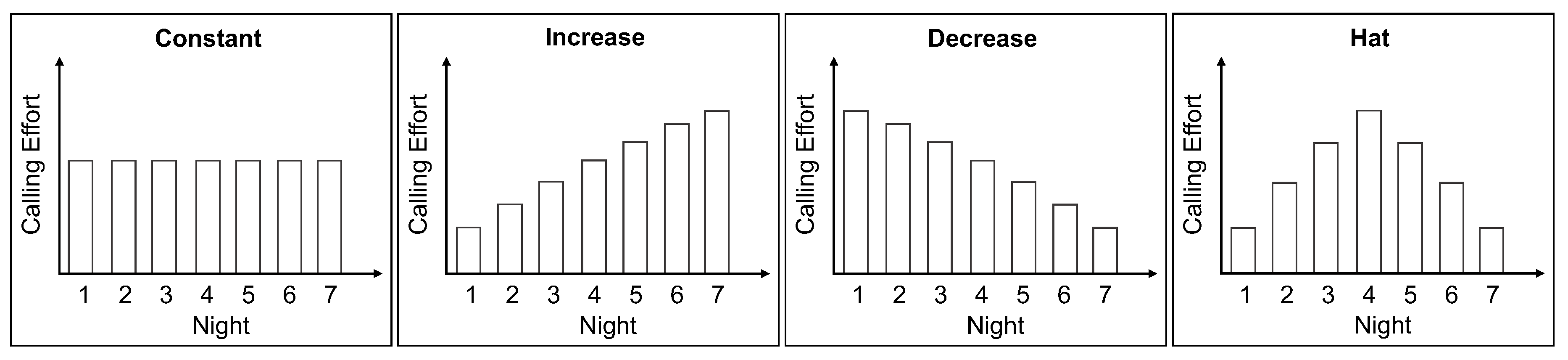
2.1. Female Calling Strategies

The release of pheromone by female moths is known as calling and is characterized by the female raising her abdomen to better disperse pheromone from the scent gland. The subsequent travel of pheromone molecules through the air forms odor plumes that are dispersed by the wind (Murlis et al. [38]). For nocturnal species, calling occurs during scotophase, the dark phase of the light–dark cycle, although the timing of calling onset, duration, and pheromone titer varies with species. Adult moths attempt to mate over several days before perishing, depending on their life span. In this section, we identify patterns of female calling and determine ranges of values for calling duration and pheromone titer. We assume a one-week mating period, as typical (Groot [7], Lees and Zilli [1]).
The meta-analysis of Umbers et al. [17] reviewed 52 empirical studies of 44 Lepidoptera species and categorized the reported female calling patterns of each. The calling effort was quantified as the time females spent calling males and/or as the amount of female pheromone titer. While most of the studies measured titer as the daily amount of chemicals present in female pheromone glands, a handful of others considered the amount of released pheromone per night. We do not distinguish between the two classifications and pool all reported values into one range. We thus implicitly assume that the amount of pheromone stored in the female body per day is the same as the cumulative amount of pheromone released during her nocturnal call. Note that it is experimentally difficult to measure pheromone ambient concentration and to infer its exact relationship to pheromone gland content (Umbers et al. [17]). Furthermore, there is great variability in the amount of pheromone stored and released by females both within a single species and across species and over the spatial extent of a pheromone plume (Mankin and Mayer [39]).
Four possible categories of female calling patterns were considered in Umbers et al. [17]: constant (the calling effort is the same every night), increase (it is greater each night compared to the night before), decrease (it is less each night compared to the night before), or hat (it increases to a peak amount and then decreases). Among those studies that measured the time that females spent calling, approximately 70% reported that the effort followed the increase pattern, 15% reported the hat pattern, 9% reported the decrease pattern, and 6% reported the constant pattern. For studies that measured pheromone titer, approximately 40% reported that the effort followed the hat pattern, 34% reported the decrease pattern, 16% reported the increase pattern, and 10% reported the constant pattern. Due to variability, our models account for changes in both the time spent calling and the pheromone titer. A schematic is shown in Figure 1.
Since our model aims to give a general picture of the dynamics of Lepidoptera moth reproduction without focusing on a single species, we group all relevant estimates reviewed in Umbers et al. [17] for calling duration (Kou and Chow [40], Mazor and Dunkelblum [41], Ming et al. [42]) and pheromone titer (Mazor and Dunkelblum [41], Ming et al. [42], Giebultowicz et al. [43], Tang et al. [44], Foster et al. [45]), to estimate the following:
  • calling duration: ranges from 0.5 to 8 h and
  • emitted pheromone: ranges from 1 to 30 ng per night.
Farrell et al. [46] estimated a pheromone release rate of 14 ng/h, corresponding to approximately 4 pg/s. As discussed above, we use these broad ranges as guiding estimates in our simulations but also consider larger values to capture the variation among species.

2.2. Male Navigational Strategies

Male moths from diverse species exhibit a set of well-known navigational behaviors in the presence of female pheromone plumes (Kennedy [30], Mafra-Neto and Cardé [31], Cardé and Willis [32], Bau and Cardé [21], Liberzon et al. [28], Benelli et al. [33]). While vertical motion is observed in the presence of trees and thick canopies and under conditions of high moth density (Girling et al. [47]), in most unobstructed cases, males stabilize their flight at a fixed altitude and motion along the vertical axis is limited (Cardé et al. [48], Elkinton et al. [49]). Male moths typically execute planar random walk flights during which their sensilla gather environmental information. Upon detection of a species-specific plume by antennal chemoreceptors, male moths orient upwind using antennal mechanoreceptors, and subsequently cease random flight and surge, flying directly upwind, towards the source.
Since turbulence of the ambient air makes pheromone plumes intermittent and filamentous, a male moth may lose contact with the plume as it surges toward the female (Martinez et al. [20]). Upon loss of pheromone signal, the moth adopts a zigzag trajectory perpendicular to the direction of wind flow at a fixed altitude. This behavior is called casting and is thought to increase the probability that the male moth would recapture the pheromone plume (Willis et al. [50]). If casting is unsuccessful for a given period of time, the male moth resumes random flight.
Estimates reported in the literature (Bau and Cardé [21], Belanger and Arabas [51], Kuenen and Cardé [52], Cardé et al. [48], Gaydecki [53]) lead us to the following male flight speed range and turning rate:
  • male flight speed: ranges from 0.5 to 5 m/s
  • male turning rate: ranges from 3 to 4 turns/s
Although flight speed and turning rates depend on whether male moths are engaged in a random flight, surging, or casting behavior, we assume that males broadly move and turn within the above ranges at all times. These values lead us to estimate typical random walk diffusivities D 1 to 10 2 m2/s, as also confirmed by other studies on Lepidoptera diffusivity estimated at D 1 to 10 1 m2/s (Watanabe [54], Kareiva [55].) For transitions between flight modes, the time necessary for males to measure pheromone concentrations is less than 100 ms, while the time to realize that the pheromone plume is lost is estimated as 300–500 ms (Stengl [5], de Bruyne and Baker [56], Baker and Vogt [57]). Since the typical time spent in any flight mode varies between seconds and hours, several orders of magnitude larger than the above awareness/decision times, we neglect the time lag between transitions. Finally, studies on pheromone-specific receptor neurons reveal that male moth sensilla are able to detect pheromones at very low concentrations, allowing for males to detect the plume at large distances (Angioy et al. [58], Tabuchi et al. [59]). If we assume a typical plume length of 2 km and estimate male flight speed at 1 m/s, we can also give the rough estimate of 30 min as the time a male moth spends in the female-generated plume. Most nocturnal male moths begin flying in the evening and until the predawn hours, indicating that male activity normally occurs away from the plume or when searching for it (Nowinszky et al. [60]).

3. Male Random Flight Model

We begin with modeling the male moth random search for the female-generated pheromone plume. This “foraging” stage of the mating process has often been considered independent of the surging/casting navigation processes, and few theoretical studies have focused on it (Cardé and Willis [32], Bau and Cardé [21], Sabelis and Schipper [61], Dusenbery [62,63]). The arrival time t a to first reach the plume however is important, since males may spend a significant portion of the night in the foraging state and since shorter arrival times are indicative of moths that are better suited for mating. Although capturing the plume necessitates finding the female through surging/casting, for simplicity, we assume here that t a is much larger than the time spent in the plume and study how the capture (and mating) probability depends on male traits relevant to random search, such as detection thresholds and diffusivity.
We utilize a two-dimensional setting with female and male moths located on the same plane at a fixed altitude based on the observed lack of male vertical motion in experimental studies, as discussed in Section 2.2. We also model the concentration of female-emitted plume c ( x , t ) as a two-dimensional field. This quantity varies in space and time, and it is a function of wind currents and female emission activity. A male moth is assumed to be able to detect the plume if c ( x , t ) is larger than a given threshold C tol , a value that indicates male chemosensitivity to pheromone and is a proxy for the length and/or elaborateness a male’s antenna, where longer/more elaborate antennae are able to sense smaller quantities of pheromone (Symonds et al. [64]).
The spatial region where c ( x , t ) > C tol defines the trapping region Ω ( t ) :
Ω ( t ) = { x : c ( x , t ) C tol } .
Once the plume is detected, the male moth will cease random flight and will surge upwind toward the female. Since lower detection thresholds C tol can be used as a proxy for male moths that are able to detect smaller amounts of pheromone and, thus, are higher quality, the trapping region Ω ( t ) is larger for higher quality males. Moths located outside the trapping region are not affected by the plume and are assumed to engage in a two-dimensional random flight with diffusion constant D, which serves as a proxy for flight speed. Similar to C tol , D can be considered an indicator of male moth quality: moths with larger D are more diffusive and are able to locate the plume earlier than moths with lower D.
We investigate how C tol and D influence t a , especially when C tol and D are both relatively large or when both are relatively small. These are interesting biological scenarios, since moths with longer and/or more elaborate antennae (smaller thresholds C tol ) are associated to larger trapping regions but are also greater in body size and less motile (smaller diffusion constants D) (Symonds et al. [64], Wang et al. [16], Johnson et al. [37]).
The probability density function g ( x , t ) that a moth is at x = ( x , y ) outside the trapping region Ω ( t ) at time t and undergoing random motion satisfies the exterior parabolic problem:
g t = D 2 g , x R 2 \ Ω ( t ) , t > 0 ,
g = 0 , x Ω ( t ) , t > 0 ,
g = δ ( x x 0 ) δ ( y y 0 ) , x R 2 \ Ω ( t ) , t = 0 ,
where x 0 = ( x 0 , y 0 ) is the initial moth location, Ω ( t ) is the dynamic trapping region defined by the time evolution of c ( x , t ) , and Ω ( t ) is its boundary. Equation (1c) implies that the moth is initially located outside the trapping region, in R 2 \ Ω ( t ) . We use absorbing boundary conditions in Equation (1b) to indicate that random flight ceases once the moth has reached the plume’s edge. At this point, the male moth will navigate toward the female using well-known surging and casting behavior. The overall probability that the moth has not captured the plume at time t is thus given by
P ( t ) = R 2 \ Ω ( t ) g ( x , t ) d x d y ,
while the overall probability that the moth has captured the plume at time t is defined as C ( t ) = 1 P ( t ) . Since we equate reaching the plume with mating success, C ( t ) can also be referred to as the moth mating probability.
One quantity of interest is the arrival time distribution S ( t ) of a moth to the trapping region (Chou and D’Orsogna [65]), which is determined by calculating the total flux:
S ( t ) = d P d t = d d t R 2 \ Ω ( t ) g ( x , t ) d x d y .
Using standard differentiation tools for the moving surface in Equation (1a) and the divergence theorem, we write the following:
S ( t ) = D Ω ( t ) g · n d + Ω ( t ) ( v b · n ) g d ,
where n is the outward facing normal vector to the Ω ( t ) boundary contour, v b is the velocity of the boundary contour element, and d is the arc length along Ω ( t ) . Equation (4) implies that the extent of trapping region Ω ( t ) is time-dependent and that its changing boundaries define non-isotropic shapes.
To follow the time evolution of Ω ( t ) we need to specify the dynamics of c ( x , t ) , which will be done in Section 5. Here, instead, we introduce some simplifications to Equation (4) which will allow for a more basic yet fundamental understanding of the mating process. We thus assume that Ω ( t ) is static and circular, centered at the origin, and characterized by a radius r mate so that the first term in Equation (4) is an integral over a circumference and the second term vanishes. We associate higher quality moths with a larger r mate (and larger D) and lower quality moths with a smaller r mate (and smaller D).
In this scenario, closed form expressions for the quantities of P ( t ) and S ( t ) can be calculated (Wendel [66], Carslaw and Jaeger [67]). Detailed derivations are given in Appendix A. We find
S ( t ) = 2 D π r mate 2 ω = 0 J 0 ( ω ) Y 0 ( ω R 1 ) J 0 ( ω R 1 ) Y 0 ( ω ) Y 0 2 ( ω ) + J 0 2 ( ω ) ω e ω 2 D t / r mate 2 d ω ,
P ( t ) = 2 π ω = 0 J 0 ( ω ) Y 0 ( ω R 1 ) J 0 ( ω R 1 ) Y 0 ( ω ) Y 0 2 ( ω ) + J 0 2 ( ω ) 1 ω e ω 2 D t / r mate 2 d ω ,
where J 0 ( z ) and Y 0 ( z ) are Bessel functions of the first and second kinds, respectively, and the dimensionless R is defined as
R = r mate x 0 2 + y 0 2 = r mate r 0 ,
and where r 0 is the male moth’s initial distance from the female. If we assume that the male moth is initially outside the circular plume, r 0 r mate , Equation (6) implies that R 1 . We illustrate some characteristic forms for P ( t ) , C ( t ) , and S ( t ) in Figure 2A and typical moth trajectories obtained through numerical simulations in Figure 2B.

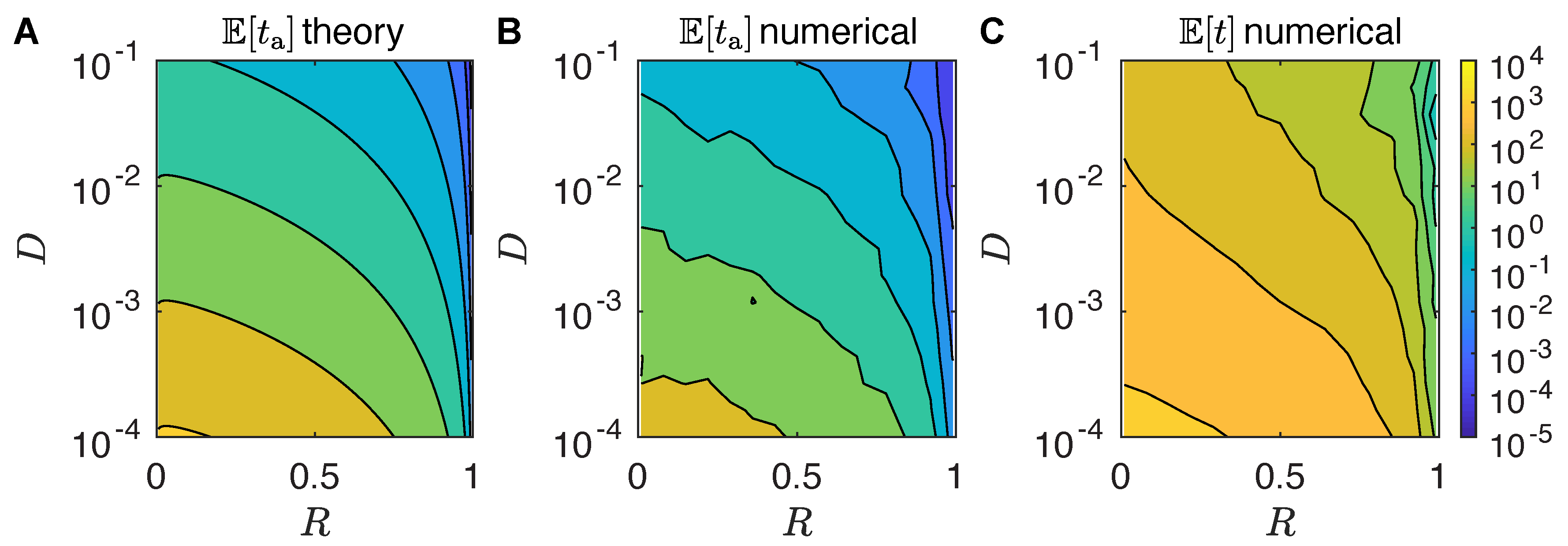
First Arrival and Mating Time

The capture/mating probability C ( t ) = 1 P ( t ) that an individual male moth reaches a female by time t and the corresponding arrival time distribution S ( t ) , evaluated via Equation (5a,b), are important overall metrics in determining the mating success of a single moth. However, competition arises when multiple males attempt to reach the same female and only the first one can mate. In this section, we consider N competing moths and adapt some known results on first arrival times (Lawley [68]) to give analytical estimates for the average time it takes the first male to reach the female. These results are valid in the N 1 limit.
In accordance with our previous discussion, we identify the male’s first arrival time to the female-generated plume as the first mating time. Lawley [68] analyzes the probability P a ( t a < t ) that the first arrival time t a out of a cohort of N independent random walkers is less than t and shows that if P a ( t a < t ) can be approximated in the short time limit as
P a ( t a < t ) A t q e B t , t 0 + ,
for a given q, A 0 , and B > 0 , then the first arrival time t a is distributed according to Gumbel distribution:
P a ( t a ) = 1 a N exp t a b N a N exp t a b N a N ,
where
a N = b N q ( 1 + W N ) , b N = B q W N , W N = W * B q ( A N ) 1 q ,
and where W * ( z ) is the principal branch of the LambertW function, defined as the inverse function of f ( z ) = z e z . The first two moments of the Gumbel distribution are
E [ t a ] = b N γ e a N , Var [ t a ] = π 2 6 a N 2 ,
where γ e 0.5772 is the Euler–Mascheroni constant.
We can use these results by noting that, within our model, P a ( t a < t ) can be identified with the capture/mating probability C ( t ) : if the first arrival time is less than t, then at time t, the moth will have reached the plume. In Equation (A20) of Appendix B, we derive the short time behavior for C ( t ) and verify that it follows Equation (7) as t 0 + . We find
C ( t ) A t q e B t , t 0 + ,
with
q = 1 2 , A = 2 ( 1 R ) r mate D R π , B = r 0 2 ( 1 R ) 2 4 D ,
from which we conclude that the average first arrival time t a for N competing male moths is given by
E [ t a ] r 0 2 ( 1 R ) 2 2 D W N 1 2 γ e 1 + W N ,
where
W N = W * 2 N 2 R π ln N .
The mean first arrival time E [ t a ] is thus a decreasing function of D and a quadratically increasing function of r 0 ( 1 R ) = ( x 0 2 + y 0 2 ) 1 / 2 r mate , as can be expected from random searchers in two dimensions. Also note that, since W N ln N , in the N limit, E [ t a ] scales as ( ln N ) 1 . Finally, note that these estimates assume that the time frame for male moths to reach the female is unbounded, so that all values of t a , including large ones, contribute to E [ t a ] as evaluated in Equation (13a). In practice, the female call may last for a limited period t call , so that arrival times t a > t call would not be tallied.

4. Numerical Results for the Male Random Flight Model

We now use a two-dimensional Brownian motion-based particle model with N independent individual male moths to numerically simulate the simplified mating process described so far. We begin with a single female call in Section 4.1 and numerically evaluate the capture and mating probabilities as well as the mean first mating time in Section 4.2. Where possible, we compare our numerical results with analytical estimates. Later, in Section 4.3 and Section 4.4, we will consider multiple calling events unfolding over a typical seven-night period with the female being able to select her mating strategy. Table 1 lists all parameters used.

4.1. Single Female Calling Period

In this section, we consider male moths responding to a single female calling period. Moths are initially placed in an equidistant manner on a circle of radius r 0 = ( x 0 2 + y 0 2 ) 1 / 2 > r mate , so that R < 1 , and undergo a random walk until the stationary, circular plume of radius r mate is reached or the total simulation time t sim elapses. We use an adaptive time stepping scheme to ensure that sufficiently small time steps (hence sufficiently small spatial steps) are taken near the plume circumference to reduce boundary errors in our simulation. If the time step is too large, the corresponding spatial step may take a free moth that starts at the exterior of the plume at time t across a short secant through the plume to an updated position that remains on the exterior of the plume at time t + Δ t . The plume flyover would incorrectly tally this moth as unsuccessful in reaching the female and would result in an underestimate of the mating probability.
The position x ( t ) of a given moth at time t is updated as
x ( t + Δ t ) = x ( t ) + 4 D Δ t r s r ^ ,
where D is the diffusion constant, r s is randomly drawn from the standard normal distribution, and r ^ is a unit vector isotropically oriented. This corresponds to a position-jump process where the mean square displacement after time T is 4 D T , as expected for two-dimensional random movement with diffusion coefficient D. As discussed above, the time step Δ t is chosen in an adaptive manner depending on the moth’s distance to the circular plume d ( t ) = ( x ( t ) 2 + y ( t ) 2 ) 1 / 2 r mate . We pose
Δ t ( d ) = ( Δ t max Δ t min ) tanh ( k d ) + Δ t min ,
so that Δ t ( d ) interpolates between Δ t min (the shortest time step) and Δ t max (the largest time step). In the vicinity of the plume, Δ t ( d 0 ) = Δ t min , whereas at sufficiently large distances, Δ t ( d ) = Δ t max . The parameter k controls the steepness of the transition between Δ t min and Δ t max . We set k = 1 m−1. A male moth is assumed to have captured the plume and to have successfully mated once d ( t ) < 0 .
We follow the trajectories of N = 5000 moths engaged in a random flight for a range of diffusivities D and mating radii r mate . All moths are initiated at an initial radius r 0 = 1 m. Simulations are halted once the simulation time t sim = 100 s has elapsed. Since the N male moths are independent, the fraction of moths to have reached the female by t sim can reasonably approximate the capture and mating probability C ( t sim ) = 1 P ( t sim ) as analytically evaluated in Equation (5b).
We find that the analytical expression in Equation (5b) and our simulation results are in good agreement for all surveyed values of D and r mate , as shown in Figure 3A, for the specific choice t sim = 100 s. The dimensionless 0 R 1 is plotted on the horizontal axis of Figure 3A instead of r mate for compactness. Larger values of R 1 indicate moths that are initiated closer to the stationary plume, whereas smaller values of R 0 indicate moths that are initiated further away from the female. A contour plot for the numerical capture and mating probability at time t sim as a function of D and R is shown in Figure 3B. Increasing the simulation time t sim yields capture and mating probabilities that approach one.
As can be seen from Figure 3A, and as can be expected, male moths with very low diffusivity are not able to reach the female within t sim unless they are initially very close to her and R 1 . At higher diffusivity, the mating probability is an increasing function of R. Figure 3B reveals the existence of a trade-off between the diffusivity and a moth’s initial distance from the female. For the capture and mating probability C ( t ) to remain fixed, decreasing R (or equivalently r mate ) requires a concurrent increase in the moth’s diffusivity D. Thus, to be competitive, moths that are less sensitive and that cannot yet sense the plume must be more agile in exploring the physical space.

4.2. First Arrival Time

We now evaluate the expected time for a male moth to first arrive at the plume. The mean first arrival time E [ t a ] is analytically estimated in Equation (13a) and is a function of male diffusivity D, plume radius r mate , and N. Numerically, it will also depend on the duration of the calling time, which poses an upper limit for the time available to males to reach the female. Here, we we set t call to be the total simulation time, t call = t sim . We repeatedly simulate independent male moths performing random flights with diffusivity D and record the time t a for each to reach the female-generated plume at r mate starting from an initial radius r 0 until the number of arrivals is N or the maximum number M of simulations is reached. For those males who are unable to reach the female within t call , no entry is tallied and the attempt is discarded and not used when calculating the mean first arrival time. If R 1 and t call is large enough, we expect the number of discarded events to be few, and a male reaching the female at times larger than t call is expected to be a rare event. However, if R 1 and t call is not large enough, many males will fail to reach the female within the allotted time. The mean first arrival time we evaluate here is thus conditioned on the male reaching the female within t call .
For most D and R parameter values, simulating N = 1000 arrivals is straightforward since the capture/mating probability C ( t ) is relatively large; however, for those parameter values with small C ( t ) , many simulations are required. When t call = 1800 s, min R , D C ( t ) 0.0175 . Thus, we choose the maximum number of simulations M = 60000 to obtain approximately M C ( t ) = 1050 > N = 1000 arrivals. From these N = 1000 arrival times, we then simply obtain the minimum and average values.
Theoretical results are shown in Figure 4A, where we present a contour plot of the mean first mating time E [ t a ] as a function of D and R based on Equation (13a). Simulation results for the mean first mating time conditioned on arrival prior to t call = t sim are presented in Figure 4B. There is good agreement between the two, indicating that moths reaching the female plume at times larger than t call are few and do not affect E [ t a ] . Ranges are E [ t a ] 10 5 to 10 3 , depending on parameter choices. In addition to the first arrival time, we also calculate the mean arrival time which is displayed in Figure 4C. As can be expected for all parameters, this quantity is larger than the expected mean first arrival time, with typical values ranging between E [ t ] 1 to 10 3 .
Figure 4 reveals that the mean first arrival and mating time E [ t a ] is lowest for moths with large diffusivity D and large values of R 1 , with mating radius r mate r 0 . Similar trends are observed for the mean arrival time E [ t ] . One key observation is that the difference between the mean first mating time and the average arrival time can be several orders of magnitude in { R , D } phase space.

4.3. Multiple Female Calling Periods

So far, females have been modeled to call males via a single calling period of time t sim . In this section, we model calling over a typical one-week period where calling times can be adjusted nightly according to the chosen constant, increase, decrease, or hat strategies described in Section 2.1 and Figure 1. The female still generates a stationary, circular plume that attracts male moths, and male quality will still be associated with large diffusivities D and large sensitivity radii r mate .
For each of the k nights, with 1 k 7 , we denote the time spent calling by t call ( k ) , while the radius of the circular plume per call is fixed at r mate . Regardless of female strategy, the values of t call ( k ) are chosen between a minimum of 0.5 and maximum of 8 h as reported in Section 2.1 from previous experimental observations, such that the total allotted total calling time T call = k = 1 7 t call ( k ) does not change among strategies. For 1 k 7 , we thus consider
Increase : t call ( k ) = { 0.5000 , 1.7500 , 3.0000 , 4.2500 , 5.5000 , 6.7500 , 8.0000 } , Decrease : t call ( k ) = { 8.0000 , 6.7500 , 5.5000 , 4.2500 , 3.0000 , 1.7500 , 0.5000 } , Constant : t call ( k ) = 4.2500 , Hat : t call ( k ) = { 2.5870 , 3.8804 , 5.1739 , 6.4674 , 5.1739 , 3.8804 , 2.5870 } .
We set r 0 = 1 m and utilize two possible values for r mate : r mate = 3 / 4 r 0 for a higher quality male and r mate = 1 / 4 r 0 for a lower quality male. Finally, male diffusivities are set at D = 10 3 / 2 or D = 10 7 / 2 m2/s, resulting in four possibilities:
{ R , D } = { 0.75 , 10 1.5 m 2 / s } , { 0.75 , 10 3.5 m 2 / s } , { 0.25 , 10 1.5 m 2 / s } , or { 0.25 , 10 3.5 m 2 / s } .
These parameter values are chosen as typical values from Figure 3.
To calculate the capture and mating probabilities C k on each night, we evaluated C k C ( t call ( k ) ) from Equation (5) with t = t call ( k ) and the four { R , D } parameters specified above. We find that the capture and mating probability C k for male moths with the highest diffusivities and the largest mating radius r mate remains elevated for all k values and relatively constant across all strategies, as can be seen in Figure 5. Moths with lower diffusivities and where r mate is smaller display capture and mating probabilities that vary with k and that follow the same trends as calling time strategy used, so that increasing calling time generally increases the mating probability from one night to the next. Intermediate capture and mating probabilities emerge for small diffusivities D but high r mate , and vice versa for large diffusivities D and low r mate , with the latter scenario yielding slightly more favorable outcomes. Figure 5 suggests that the increase or hat strategies may be best for a female to successfully attract a high-quality male through the least calling effort while still finding a mate within the one-week mating period. At onset of the mating process, both the increase or hat strategies yield a large capture and mating probability for high-quality males, with high D and large r mate , and a relatively lower probability for low-quality males, with low D and small r mate . At this stage, the female employs short calling times t call ( k ) , ensuring that she is being selective while minimizing her calling effort. As the mating period continues and t call ( k ) increases, the likelihood of attracting lower quality males increases, so that overall mating success with males of any quality increases. This observation is consistent with field observations where it is shown that female moths preferentially employ the increase strategy to optimize their mating likelihood (Umbers et al. [17]).
We confirmed that the increase and hat strategies are the most effective for females. To do so, we defined the effectiveness of the strategy on the kth night, E k , as the ratio of the cumulative total mating probability and total time spent calling (Figure 6). Using the calling times t k specified above for each strategy, we calculated the mating probability C k = C ( t k ) in the { R , D } parameter plane as in Figure 3B. This defines the total mating probability M k , which is calculated as the sum of C k over all R and D values. The effectiveness is thus calculated as the ratio of the cumulative total mating probability to the total time spent calling
E k = i = 1 k M i i = 1 k t i .
In Figure 6, we plot ( i = 1 k t i , E k ) for each night k = 1 , , 7 and for each strategy. The results show that the increase strategy is the most effective, since a female employing this strategy has high total mating probability obtained with a relatively short calling time. On the other hand, the decrease strategy is the least effective, since a female has a higher total mating probability than in the increase strategy at the cost of a long calling time.

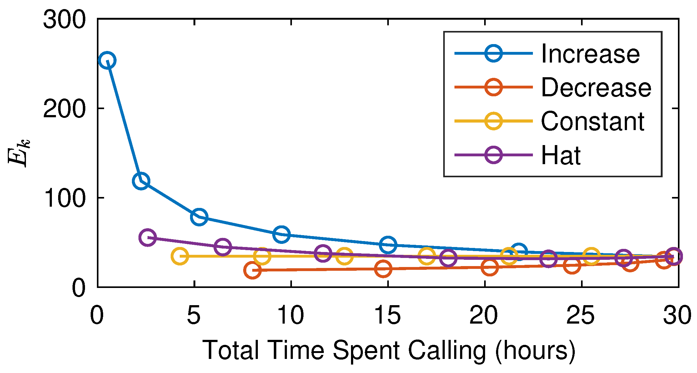
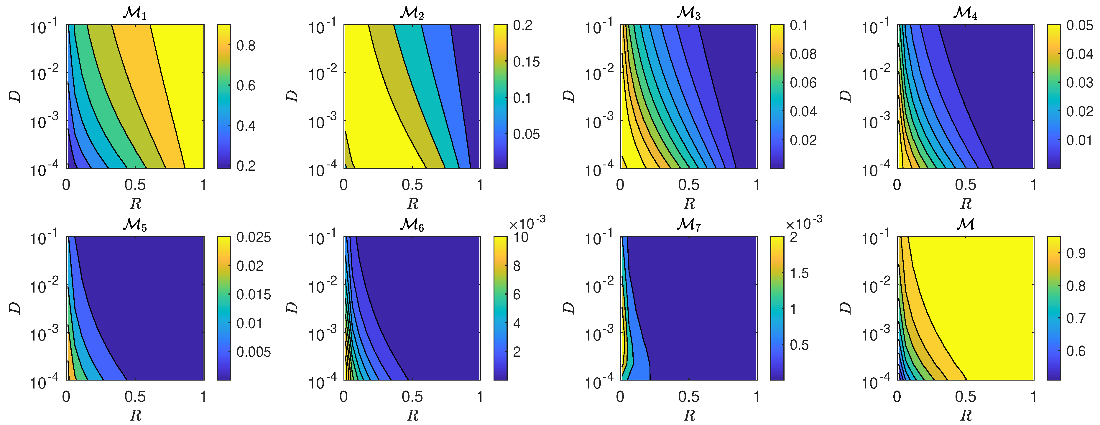
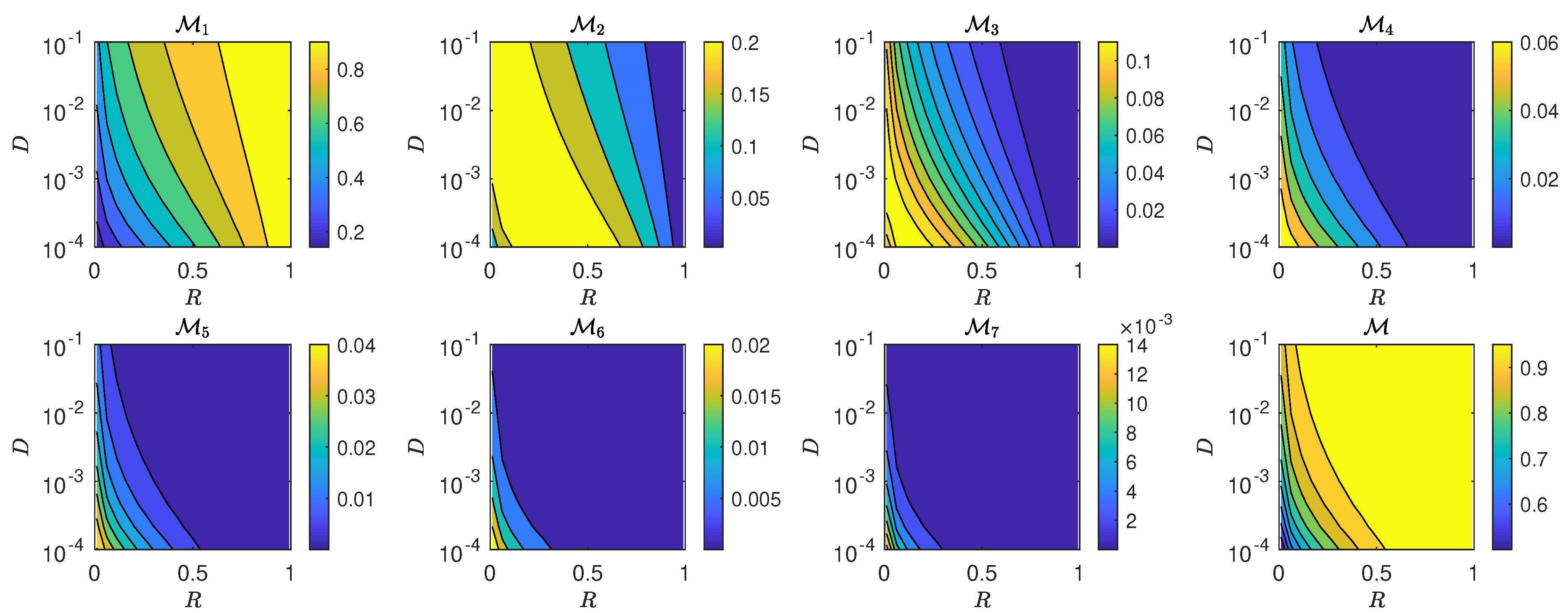
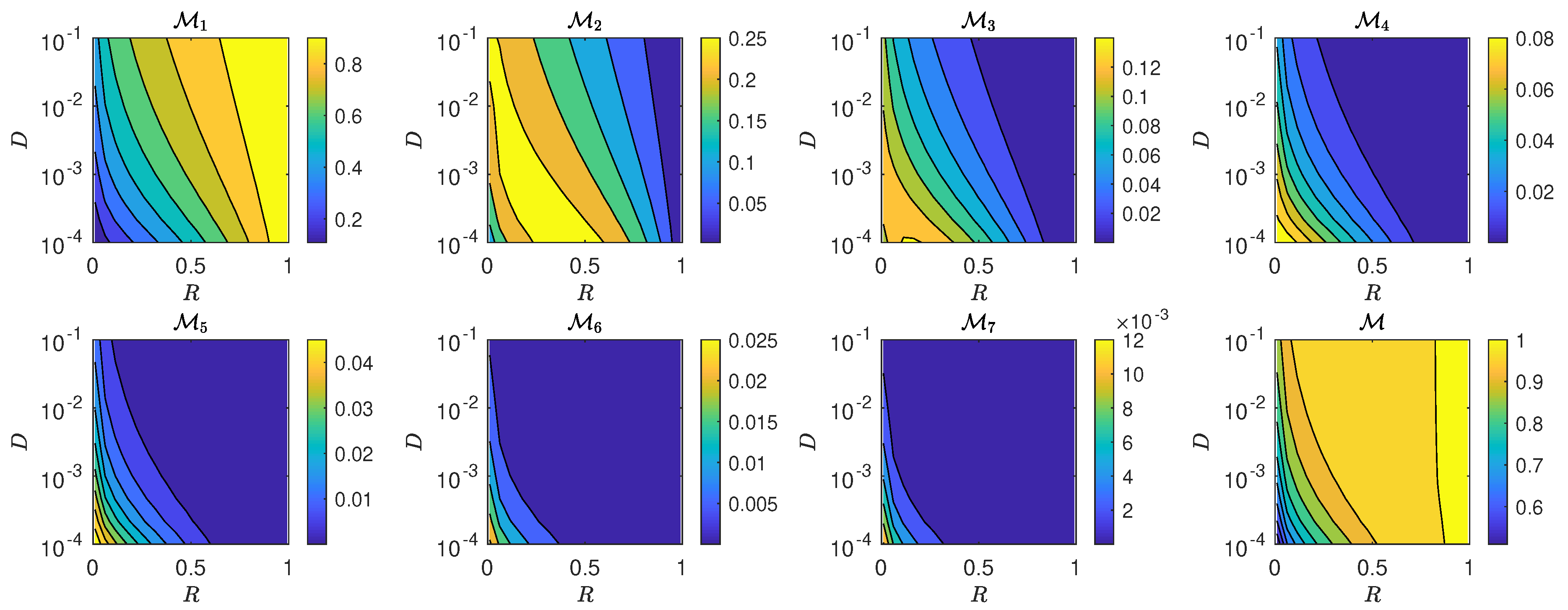
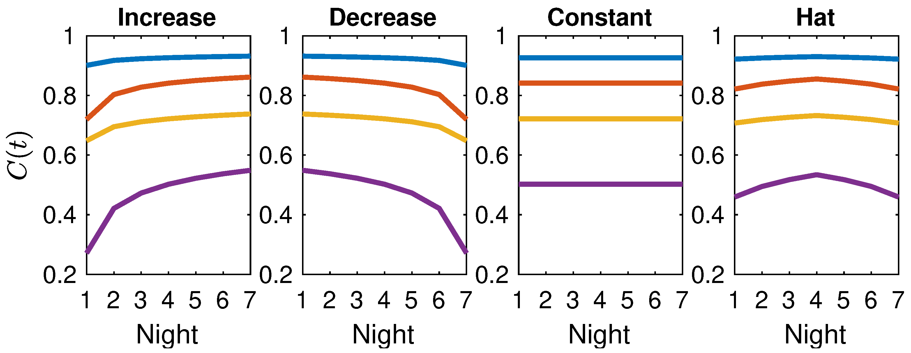
4.4. Night-by-Night Mating Probabilities

For a more nuanced understanding of the mating process, we study the night-by-night mating probability for each of the four strategies shown in Figure 5. We use the same calling time sequences t call ( k ) as in Section 4.3 but consider a wider range of values for the male characteristics R and D. In particular, we evaluate the mating probability M that a female mates on night given that no male reached her on prior nights, defined as follows:
M 1 = C 1 ,
M = C k = 1 1 ( 1 C k ) , = 2 , 7 .
We also calculate the total mating probability M over the one-week mating period given by
M = C 1 + C 2 ( 1 C 1 ) + + C 7 k = 1 6 ( 1 C k ) = j = 1 7 C j k = 1 j 1 ( 1 C k ) .
The results are shown in Figure 7, Figure 8, Figure 9 and Figure 10. We find that all four calling strategies result in qualitatively similar trends for M . Specifically, the mating probability for the first night, M 1 , is an increasing function of D and R and is largest for high-quality moths, as can be expected. However, the maximum probability on successive nights, M with > 1 , declines in magnitude and shifts to lower diffusivity D and smaller relative radius R. Compared to high-quality moths, those with medium { R , D } do not display a large mating likelihood on the first night; however, their mating likelihood remains relatively large on successive nights. This implies that, if only intermediate quality males are present, the female can increase her mating likelihood and partner with one of them if the call extends further than one night. The last panels of Figure 7, Figure 8, Figure 9 and Figure 10 show the total mating probability, M , at the end of the one-week mating process, confirming that mating occurs with large probability for almost all moth qualities considered. This suggests that a female moth can employ a conservative strategy such as the increase strategy to maximize the quality of a mate early in the calling process without risking not copulating at all after the one-week mating period.

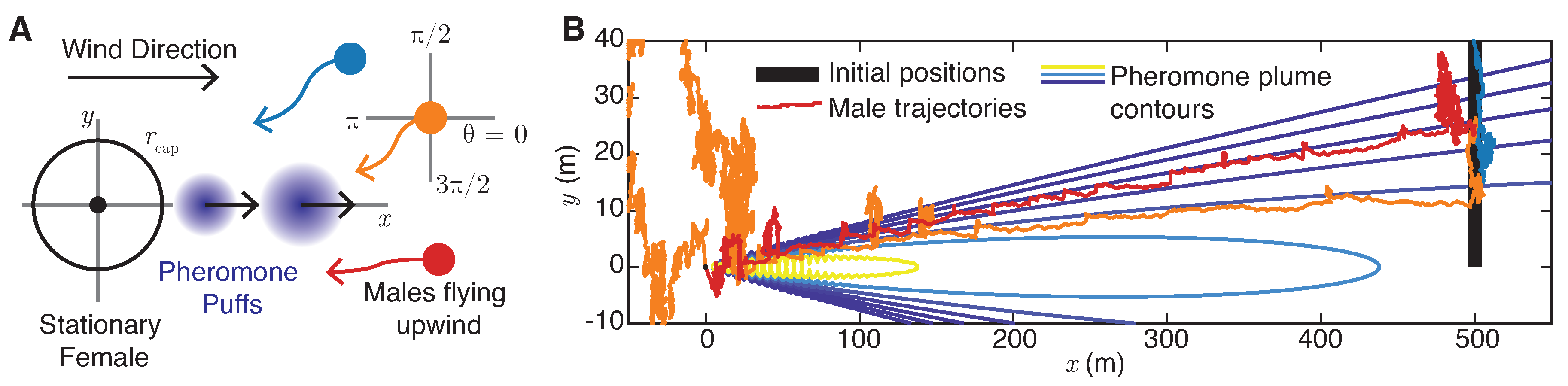
5. Plume Navigation Model

We now present an agent-based model of moth mating, called the Plume Navigation Model, where a stationary female emits pheromones and males navigate to find her. As discussed in Section 2.2, plume dynamics and moth flight are modeled in two dimensions since males typically fly at constant altitudes, whether engaged in random flight, surging, or casting behavior. Rather than considering a stationary, circular plume, as done so far, the static female is now assumed to emit a series of pheromone puffs, defining a plume that evolves according to known atmospheric dispersion models, while males search for the plume and fly through it (Cardé [69], Arbas et al. [70], Baker et al. [71], Willis et al. [72], Witzgall [73], Kaissling [74]).
Our Plume Navigation Model is based on previous work by Liberzon et al. [28] and Benelli et al. [33], who developed MothPy [75], an open-source package to simulate moth mating. While the focus of their work was to study male navigational strategies, we developed our Plume Navigation Model to investigate female calling strategies, in particular, by varying the amount of emitted pheromone and its distribution over a typical mating period of seven nights. A schematic of the Plume Navigation Model with typical male trajectories and female pheromone plume dispersion is given in Figure 11, and Table 1 lists all parameters used. Details of the Plume Navigation Model setup are given in Section 5.1 and Section 5.2 and the results are discussed in Section 5.3.

5.1. Male Navigation Algorithm

As originally formulated, MothPy [75] focuses on the latter stage of the male search for a female. Male moths are initially stationary, positioned downwind of the female, and do not actively search for the plume. Rather, the plume will diffuse and be advected toward them. Once a sufficient amount of pheromone reaches the male moths, they start moving upwind, toward the female. Thus, the random flight mode described in Section 2.2 is not employed in MothPy. Conversely, our Plume Navigation Model considers a full night of calling where the male random flight mode is included and where several female strategies are implemented.
We define our coordinate system x = ( x , y ) with the female moth at the origin and several, noninteracting, male moths initially positioned downwind of her as shown in Figure 11A. In addition to male moth movement, we track the concentration of pheromone c ( x , t ) released by the female moth as it diffuses and is convected by wind. We assume that the wind velocity field U is uniform along the positive x direction so that U = ( U ( x , t ) , V ( x , t ) ) = ( U , 0 ) , where U is a constant. Male moths are assumed to move at a constant flight speed v so that the motion of a moth at location x = ( x ( t ) , y ( t ) ) is updated at every time step Δ t via
x ( t + Δ t ) = x ( t ) + v Δ t cos θ ,
y ( t + Δ t ) = y ( t ) + v Δ t sin θ ,
where θ [ 0 , 2 π ) is the angular direction of moth movement, as measured from the x axis. Upwind movement thus occurs along θ = π , while casting occurs along θ = ± π / 2 . We also assume that the pheromone plume can be sensed by a male moth only if it is locally present at a large enough threshold concentration C tol . The algorithm for updating θ for a moth at position x is as follows:
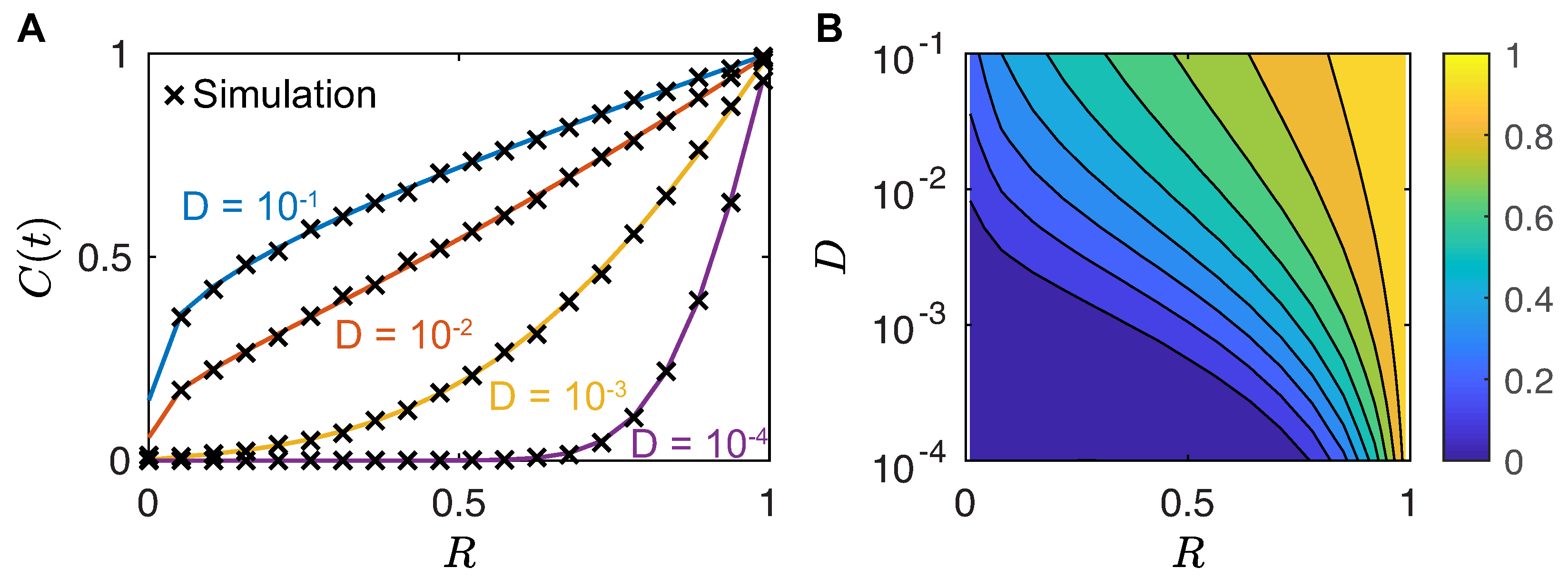
  • Random flight: If the male moth does not detect pheromone ( c ( x , t ) < C tol ) and has never detected pheromone at earlier times t < t , the moth chooses a random direction θ drawn uniformly from [ 0 , 2 π ) . Note that this motion implies that, overall, the moth executes a random flight with effective diffusivity D v 2 Δ t / 4 . For the experimentally measured male flight speeds reported in Section 2.2, v = 0.5 to 5 m/s, and for Δ t = 1 s, this corresponds to D 1 to 10 2 m2/s.
  • Surging: Upon detection of pheromone signals for c ( x , t ) C tol , the moth will align with the upwind direction of airflow ( θ = π ) with a margin of error ϵ . The updated direction of moment θ will be selected uniformly from ( π ϵ , π + ϵ ) at each timestep.
  • Casting: Upon loss of contact with the pheromone plume for c ( x , t ) < C tol , the moth will search for the plume perpendicular to the direction of airflow ( θ = ± π / 2 ) with a margin of error ϵ . The updated direction of movement θ will be selected uniformly in ( π / 2 ϵ , π / 2 + ϵ ) or in ( π / 2 ϵ , π / 2 + ϵ ) at each timestep. If the male moth is unable to find the lost pheromone plume after casting for a given time t cast , it returns to random flight mode. Otherwise, it returns to surging. Typical total casting times are on the order of 10 s (Martinez et al. [20]), so we choose t cast = 10 s.
  • Mating: Once the male moth is within a radius r cap of a female, the two successfully mate.
Example male moth trajectories exhibiting each movement mode (random flight, surging, casting, and mating) are shown as colored trajectories in Figure 11B.

5.2. Female-Generated Pheromone Plume Dynamics

The dynamics of the female-generated pheromone plume dispersing in turbulent wind is evaluated in MothPy [75] via the open source package PomPy (Graham [76]), based on the model of Farrell et al. [46]. We implement a simplified version of its dynamics in our Plume Navigation Model. Here, a stationary female moth, located at the origin, emits a series of i pheromone puffs at time t i , where i = 1 , , n . Each puff contains m i pheromone, contributes to the overall plume as a spreading Gaussian centered at x p ( t ) = ( x p ( t ) , y p ( t ) ) , and is characterized by a time-dependent diffusivity σ i ( t ) = σ 0 ( t t i ) relative to the turbulent diffusivity. The x p ( t ) center of each Gaussian may change in time, as advected by the wind velocity field U = ( U , 0 ) . The overall plume concentration c ( x , t ) at position x = ( x , y ) and at time t may thus be written as a superposition of diffusing terms originating from each of the i puffs as follows:
c ( x , t ) = i = 1 n H ( t t i ) m i 2 π σ i ( t ) 2 exp | x x p ( t t i ) | 2 2 σ i ( t ) 2 ,
where H is the heaviside function and x p ( t ) is advected by the wind velocity field so that, at each time step,
x p ( t + Δ t ) = x p ( t ) + ( U , 0 ) Δ t .
The various female calling strategies can be incorporated by selecting the proper t i sequences as well as the amount of pheromone released per puff m i .

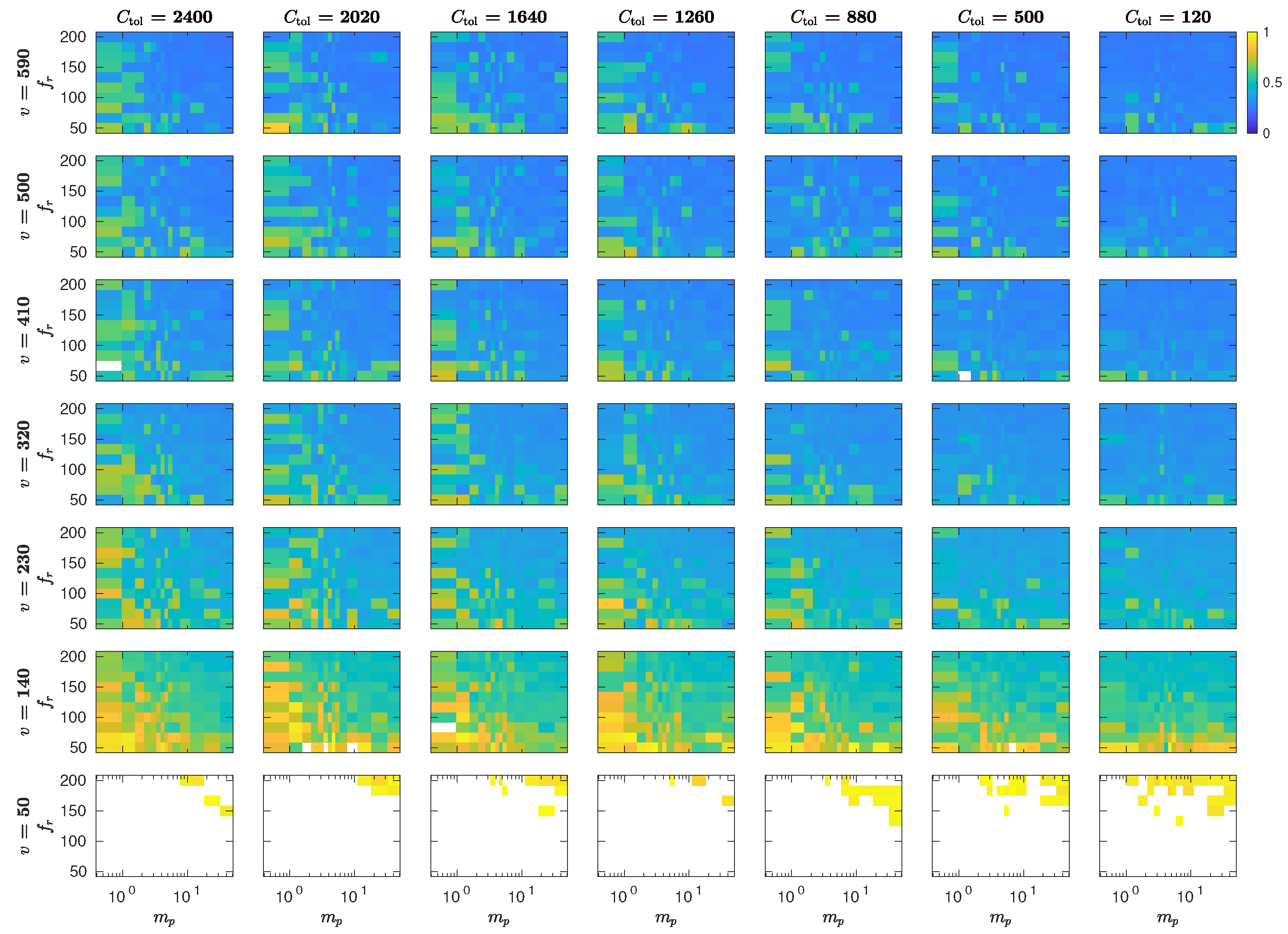
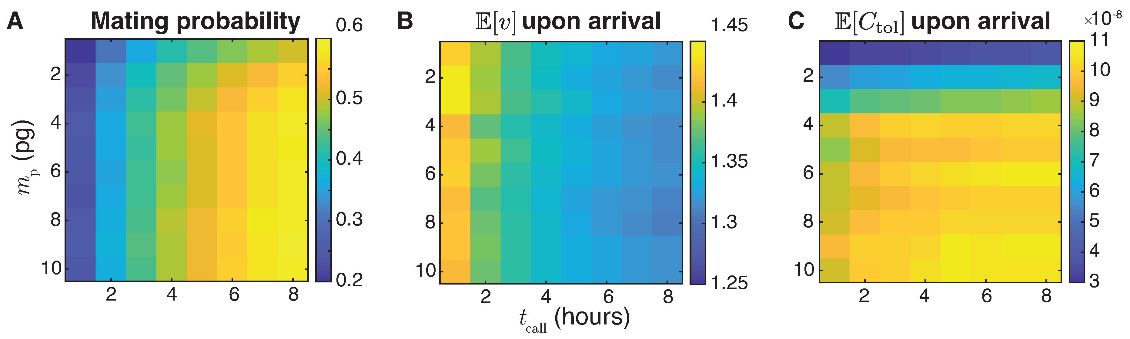
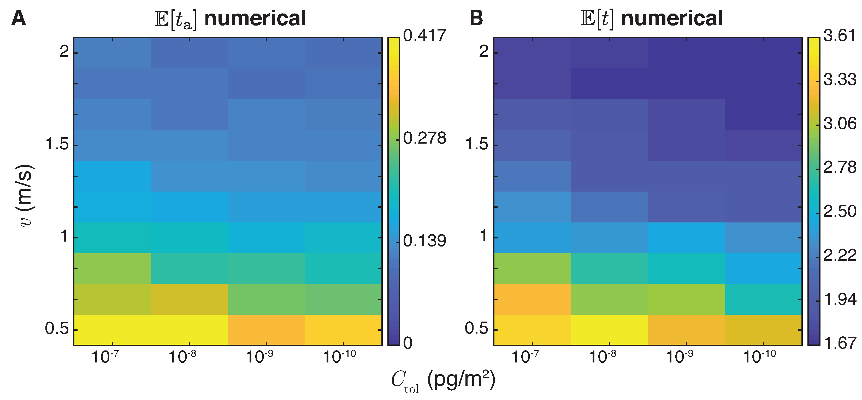
5.3. The Interplay of Calling Time and Pheromone Amount on Male Fitness

In this section, we consider the full mating problem with a stationary female generating the dynamically evolving plume c ( x , t ) presented in Equation (21). The N independent males seeking the female follow the plume according to Equation (20) and are characterized by a detection threshold C tol and a speed v; low C tol and large v represent high-quality males. We study the mating process for a wide range of calling times and released pheromone amounts.
In our simulations, the female is located at the origin and the N = 10000 non-interacting male moths are initialized 500 m downwind of her within a 100-m line perpendicular to the direction of the wind flow as shown in Figure 11B. We assume mating occurs once the male is within r cap = 5 m from the female. Once this distance is reached, the moth arrival time is recorded and the moth is removed from the simulation. Given the relatively large value of r cap , we do not adaptively change the time step Δ t at the boundary of the female-generated plume (as in the simplified model) but keep it fixed. To represent male phenotypic variability, each male is assigned a C tol value uniformly sampled in logarithmic space between 10 10 and 10 6 pg/m2 and a flight speed v uniformly sampled between 0.5 and 2 m/s.
To simulate different female calling strategies, calling times t call were varied from 1 to 8 h. Within each strategy, the emitted pheromone per puff was kept fixed at m i = m p and the puffs were emitted throughout the simulation at the rate of 1 puff per second. The m p range we used across strategies was varied between 1 and 10 pg, corresponding to overall emitted pheromone of roughly 2 ng (1 pg emitted over a 30 min call) and 300 ng (10 pg emitted over an 8 h call), exceeding the range of typical values presented in Section 2.1. Each simulation represents one night of calling. Note that, since male moths are independent, concurrently simulating the arrival of N moths is equivalent to N simulations to study the arrival of a single moth. Finally, whereas moth quality in Section 3 was represented by { R , D } , here, moth-quality indicators are { C tol , v } .
In Figure 12A, we show how the mating probability (the fraction of the N males that reach the female for all { C tol , v } values), depends on the calling time t call and emitted pheromone m p . Simulations are run over the maximum calling time t sim = 8 h when the female call ends. We then tally the total number of males that arrived from the onset of the simulation up to time t call where t call = 1 , , 8 h and compute all relevant statistics associated to t call , such as mating probability, mean speed, and mean chemosensitivity threshold. The results shown in Figure 12A thus represent cumulative subsamples of the maximum t call = 8 h call. As can be seen, the mating likelihood is much more sensitive to t call than to m p , as it increases only by approximately 10% over a tenfold increase in m p . This is in agreement with experimental observations where doubling the effective titer on a moth trap does not substantially affect the number of males that are captured (Johnson et al. [37]).
Figure 12B shows the mean speed of successful males, regardless of C tol . This panel reveals that, by tuning t call , females may preferentially select for males with different speeds: calling for a relatively short time each night (0.5 h) selects for faster males on average, while calling for full night (8 h) gives slower males the opportunity to mate (Figure 12B). Similarly, Figure 12C displays the mean detection threshold of successful males, regardless of v. This panel shows that modulating pheromone titer m p is an avenue for females to select for males with lower C tol that are able to sense smaller pheromone concentrations. If we assume that lower C tol is a proxy for longer antennae in moths, our findings are consistent with experimental observations where doubling the effective titer on a moth trap leads to capture of males with smaller antennae (Johnson et al. [37]).
In Figure 13A we show the mean first arrival times in { C tol , v } phase space for a fixed pheromone titer m p = 1 pg and calling time t call = 8 h. As can be seen, the fastest and most chemosensitive males display the shortest mean first arrival times; vice versa, the slowest and least sensitive males display the longest mean first arrival times. Similar trends are seen in Figure 13B, where instead, we plot the mean arrival and mating time. These findings are in qualitative agreement with the simplified male random flight model where moths with the largest diffusivity D and largest ratio R = r mate / r 0 are the first to reach the female and display the lowest mean arrival times.
Finally, to compare our Plume Navigation Model to existing models, we used MothPy [75] to quantify the fraction of successful males and minimum arrival times as a function of female calling strategies (pheromone puff release rate and molecular amount) and male quality parameters (speed and pheromone detection threshold). The main trends regarding the relationship between female calling and male quality with reproductive success are similar to those obtained via our Plume Navigation Model as discussed in the previous three paragraphs; details of the MothPy simulations can be found in Appendix C.

6. Discussion

In this work, we studied different sexual selection methods used by female moths to attract males with high-quality traits: faster flight speed/diffusivity and better ability to sense small concentrations of pheromone, i.e., chemosensitivity. Specifically, we considered four experimentally observed calling strategies where the female varies calling times and amounts of emitted pheromone over a one-week period in an attempt to optimize both mating success and quality of the first male to mate. Since male moth navigation and pheromone dynamics typically occur at fixed altitude, we only considered two-dimensional representations.
We developed an initial simplified agent-based model (the Male Random Flight Model) where the female-generated pheromone plume is assumed to be static and circular and male moths are assumed to be random walkers before reaching the plume, which allowed us to find analytical estimates for the mean first arrival time. We considered a cohort of N independent males, with diffusion constant D, who can sense the female-generated plume at a distance r mate that started at a distance r 0 > r mate from the female. For a single calling period of fixed duration, the mean first arrival is found to scale as E [ t a ] ( r 0 r mate ) 2 / ( D ln N ) . We identified r mate and D with male quality: large values of r mate indicate moths that sense the female at larger distances, and large values of D indicate moths that can more readily explore the environment. An interesting avenue for future research would be to extend these results to a variety of random walk models such as those analyzed in Petrovskii et al. [77] and in Bläßle and Tyson [78]. We also considered multiple calling periods distributed over seven nights according to an increase, decrease, hat, or constant pattern such that the total possible calling time, which is a measure of effort on the female’s part, remains constant across strategies. We find that the optimal calling strategy that minimizes expenditure while maximizing male quality and overall mating likelihood is the increase strategy, as has also been shown by experimental studies.
Our more complex agent-based model (the Plume Navigation Model) allowed us to include realistic female-generated plumes that evolve dynamically due to advection by wind and atmospheric dispersion over timescales of several hours. Male navigation is modeled in a more detailed manner: prior to sensing the plume, males are assumed to perform Brownian motion; once the pheromone is detected, they surge upwind toward the female. If the plume is lost, the moth will engage in casting behavior to relocate the plume. At the end of the casting phase, if the pheromone remains undetected, the moth will return to performing Brownian motion, else it will surge toward the female. We used the pheromone detection threshold of male moths, C tol , and their diffusive velocity v as proxies for male quality. Finally, we allowed male moths to search for the female plume over realistic periods of up to eight hours per night.
Where possible, we used experimental studies to inform parameter values. Ideally, a female reproduces at the beginning of adulthood with a high-quality male; however this may not always be possible and the female may need to adjust her calling strategy to attract males of lesser quality before the mating period ends. Our models confirm that, if a female initially releases limited quantities of pheromone m p per puff and the calling time t call is brief, only the more motile and chemosensitive males may reach her. Mating likelihoods for moths of lesser quality improve once the amount of released pheromone or calling time increases. We found that the mean first capture and mating times and the mean arrival times can differ by several orders of magnitude, indicating that pheromone-based signaling may help balance the goal of selecting a high-quality male versus the need to mate within a finite time.
We find that overall mating likelihood is more sensitive to t call than to m p but that modulating m p allows the female to select for higher quality males with lower pheromone detection thresholds C tol . If we associate more chemosensitive males with lower C tol levels to males with longer antennae, these findings are consistent with experimental observations where doubling the effective titer on a moth trap does not change the overall abundance of captured moths, but the antennae of males captured by single-female traps were observed to be longer than the antennae of males captured by double-female traps (Johnson et al. [37]). Simulations using MothPy performed over a 20-s timeframe when males are in close proximity to the female also confirm these findings, as shown in Appendix C.
Antenna structure is an evolutionary aspect of moth anatomy. While some species display large, branching antennae to maximize surface area, sensilla count, and pheromone detection (Symonds et al. [64], Wang et al. [16]), phylogeny shows that a majority of moths have simple non-branching antennae to minimize aerodynamic drag during flight (Symonds et al. [64]). In this case, sensilla and scales are carefully arranged so that chemical detection, pheromone retention, and flight capabilities are concurrently optimized (Wang et al. [16]). Greater power and strength allow moths to sustain large antennae and elevated speeds, so that moth body and antenna sizes are often correlated (Johnson et al. [37]). Our results indicate that maintaining the same mating probability when pheromone detection thresholds decrease (so that the male is more chemosensitive) requires the male flight speed to decrease.
Our models include several simplifying assumptions about moth behavior and interactions. For example, we consider the behavior of many independent males and a single calling female. These models could be expanded to study multiple females simultaneously emitting pheromones and their effects on male selection. Would female–female competition alter the optimal female strategies? There is also evidence that, in some species of moths, female calling attracts conspecific females as well as males (Su et al. [79]). This may lead to spatial clusters of females, which in turn produce larger aggregate plumes capable of attracting more males and males with higher C tol . This is another aspect of female–female behavioral interaction that may alter optimal female strategies. While our models assume that females mate only once and that the first male to reach the female mates with her, additional male–male competitive behaviors (e.g., multiple mating and spermatophore displacement) could be incorporated (Xu and Wang [34]). For species that engage in multiple mating, these behaviors may substantially change the selection pressures and female strategies as the last male to mate, rather than the first, would be considered the successful male. Additionally, while our models were built with a general moth in mind, species-specific parameter values could be used in cases where sufficient experimental data is available.
When studying the Male Random Flight Model, we made the simplifying assumption for mathematical convenience that the plume is a static circle of radius r mate . We thus focus on the “foraging” part of the mating process where the male searches for this static circular plume. This simplifies the mathematical analysis carried out in Section 3 but does ignores the physical fact that the plume is dynamic and is affected by the environment. An extension to our work could be to consider a dynamic trap radius that increases over time r mate ( t ) that coarsely captures the plume’s spread. Although our results are focused on the random movement of individual moths and female calling strategies, it may also be insightful to compare the mean results of many stochastic simulations with the solution to a continuum model describing the chemotaxis-diffusion of male moths and reaction-convection-diffusion of the female pheromone plume. The construction of such a continuum model would require detailed consideration of the distinct modes of male movement (random, surging, casting, and mating) and whether the males undergo position or velocity jumps (Othmer et al. [80]).
There are many aspects of moth life dynamics that may also play a role in the mating process. We studied the mating process over seven nights of calling—a typical moth lifespan. However, other life dynamics such as death rates may be important considerations in future work. Ecologically, moths play a fundamental role near the bottom of the food chain, acting as prey for bats, birds, and other small mammals. Tcheslavskaia et al. [81] estimated that the mortality of female gypsy moths due to predation ranges between 0 to 35% per night, with an average of 14.2 ± 2.5% fatalities per night.
Another possibility is to study hybrid mating. Here, multiple moth strains could be introduced, each responding to a specific pheromone blend, for which the chemical components are expressed in tightly controlled ratios that define blend-specific diffusion and decay rates. These blends allow only moths of the same strain to recognize one another. Although males will initially follow the blend from their own strain, when plumes overlap they may eventually relax their specificity and begin following plumes from other strains, leading to hybrid mating (Kárpáti et al. [82]).
While moths are efficient pollinators (Walton et al. [83]), some species are considered major agricultural pests, and environmentally safe pest control procedures are wanting. For example, mating disruption is a method of releasing formulated synthetic copies of female pheromone that drive males to traps and curb reproduction (Cardé and Minks [84], Barclay and Judd [85], Gordon et al. [86], Lucchi et al. [87]). There is an opportunity for computational simulations, such as those presented in this work, to provide additional information that experiments cannot, as comprehensive field studies are difficult and existing data is sparse. To improve mating disruption methods, minimizing the amount of synthetic pheromone released from automatic devices can reduce costs, both economic- and health-related. Our computational Plume Navigation Model provides information on the effects of female calling strategies which can help inform the timing and length of synthetic pheromone release in mating disruption.

Supplementary Materials

The computer code used to generate the results for this article is available through GitHub at https://github.com/tstepien/moth-mating [v1.0.0]. The code is platform independent and written in MATLAB, which requires a license, and Python.

Author Contributions

Conceptualization, M.R.D. and A.E.L.; methodology, T.L.S., C.Z., J.B.H., R.M.C.R., M.R.D., and A.E.L.; software, T.L.S., C.Z., J.B.H., and A.E.L.; validation, T.L.S., C.Z., J.B.H., M.R.D., and A.E.L.; formal analysis, T.L.S., C.Z., J.B.H., M.R.D., and A.E.L.; writing—original draft preparation, T.L.S., C.Z., J.B.H., R.M.C.R., M.R.D., and A.E.L.; writing—review and editing, T.L.S., C.Z., J.B.H., R.M.C.R., M.R.D., and A.E.L.; visualization, T.L.S., C.Z., J.B.H., and A.E.L.; supervision, M.R.D. and A.E.L.; project administration, T.L.S., M.R.D., and A.E.L.; funding acquisition, M.R.D. and A.E.L. All authors have read and agreed to the published version of the manuscript.

Funding

This material is based upon work supported by the National Science Foundation under grant numbers DMS 1641020 (AMS MRC program), DMS 1562078 (C.Z.), DMS 1815216 (A.E.L.), and DMS 1814090 (M.R.D.); by the Army Research Office under grant numbers W911NF-18-1-0345 and W911NF-16-1-0165 (M.R.D.); and by a Natural Sciences and Engineering Research Council of Canada (NSERC) Postdoctoral Fellowship Award (C.Z.). This work was conducted in part using the resources of the Advanced Computing Center for Research and Education (ACCRE) at Vanderbilt University, Nashville, TN.

Acknowledgments

We wish to acknowledge the American Mathematical Society’s Mathematical Research Community (MRC) in Agent-Based Modeling in Biological and Social Systems, which brought our collaboration together and supported our work.

Conflicts of Interest

The authors declare no conflict of interest.

Appendix A. Derivation of Arrival Time to Circular Plumes

In this appendix, we evaluate the arrival time distribution for a two-dimensional random walker to reach a trapping disk of radius r mate , i.e., Ω = { ( x , y ) x 2 + y 2 r mate 2 } . In Cartesian coordinates, the probability density function g ( x , y , t ) for a walker to occupy position x = ( x , y ) solves the parabolic exterior problem:
g t = D 2 g , x 2 + y 2 > r mate 2 , t > 0 ,
g = 0 , x 2 + y 2 = r mate 2 , t > 0 ,
g = δ ( x x 0 ) δ ( y ) , x 2 + y 2 > r mate 2 , t = 0 .
Without loss of generality, in Equation (A1b) we set the initial location of the moth to be at ( x 0 , 0 ) , so that its distance from the female is r 0 = x 0 . To solve Equation (A1), it is convenient to first transform to dimensionless variables and a polar coordinate system. Accordingly, we write
x = r mate r cos θ , y = r mate r sin θ , t = r mate 2 D τ , R = r mate r 0 , g ( x , y , t ) = p ( r , θ , τ ) ,
so that the problem for p ( r , θ , τ ) satisfies
p τ = p r r + 1 r p r + 1 r 2 p θ θ , r > 1 , θ [ 0 , 2 π ) , τ > 0 ,
p = 0 , r = 1 , θ [ 0 , 2 π ) , τ > 0 ,
p = R δ ( r R 1 ) δ ( θ ) , r > 1 , θ [ 0 , 2 π ) , τ = 0 .
The solution to Equation (A2) is now determined with the goal of developing closed form expressions for the following three quantities:
Probability   moth   still   free   at   time τ : P ( τ ) = θ = 0 2 π r = 1 p ( r , θ , τ ) r d r d θ , Probability   moth   trapped   by   time τ : C ( τ ) = 1 P ( τ ) , Arrival   time   distribution   of   moths   to   trap : S ( τ ) = P ( τ ) .
The solution begins by defining the Laplace transform:
p ^ ( r , θ ; s ) = τ = 0 p ( r , θ , τ ) e s τ d τ , s C .
The quantity p ^ ( r , θ ; s ) satisfies the associated elliptic equation:
p ^ r r + 1 r p ^ r + 1 r 2 p ^ θ θ c 2 p ^ = R δ ( r R 1 ) δ ( θ ) , r > 1 , θ [ 0 , 2 π ) ,
p ^ ( 1 , θ ) = 0 , θ [ 0 , 2 π ) ,
where c 2 = s . In practice we are only interested in the radial component of the solution which describes the arrival time distribution. For completeness, we describe the full solution obtained by seeking a separable solution of Equation (A4) that is continuous, periodic, even in θ , bounded as r , and satisfies the boundary condition p ^ = 0 on r = 1 . This series is
p ^ ( r , θ ) = n = 0 A n I n ( c r ) I n ( c ) K n ( c ) K n ( c r ) cos ( n θ ) , r < R 1 , n = 0 A n I n ( c R 1 ) K n ( c R 1 ) I n ( c ) K n ( c ) K n ( c r ) cos ( n θ ) , r R 1 ,
where A n are constants to be found from incorporation of the Dirac source term. The functions I n ( z ) and K n ( z ) are modified Bessel functions of the first and second kinds, respectively. Multiplying Equation (A4) by cos ( m θ ) and integrating over ( r , θ ) ( R 1 ε , R 1 + ε ) × [ 0 , 2 π ) , we find in the limit as ε 0 that
lim ε 0 r = R 1 ε R 1 + ε θ = 0 2 π cos ( m θ ) r r p ^ r d r d θ = 1 .
The orthogonality of { cos m θ } m = 0 over [ 0 , 2 π ) yields the jump condition
A n c R θ = 0 2 π cos 2 ( n θ ) d θ I n ( c R 1 ) K n ( c R 1 ) I n ( c ) K n ( c ) K n ( c R 1 ) I n ( c R 1 ) + I n ( c ) K n ( c ) K n ( c R 1 ) = 1 .
The jump condition (A7) can be simplified with the Wronskian identity
K n ( z ) I n ( z ) I n ( z ) K n ( z ) = 1 z ,
to find that
A n = K n ( c R 1 ) θ = 0 2 π cos 2 ( n θ ) d θ 1 = K 0 ( c R 1 ) 2 π , n = 0 , K n ( c R 1 ) π , n 1 .
The Laplace transform of the flux over the disk is then given by
p ^ r | r = 1 = n = 0 A n K n ( c ) cos ( n θ ) = 1 2 π K 0 ( c R 1 ) K 0 ( c ) + 1 π n = 1 K n ( c R 1 ) K n ( c ) cos n θ .
Returning to the variable to s = c , we now apply the inverse Laplace transform of Equation (A10) and evaluate the contour integrals:
1 2 π i Γ K n ( s R 1 ) K n ( s ) e s τ d s , n = 0 , 1 , 2 , ,
where the integral is evaluated over the complex curve Γ = { γ + i y | y ( , ) } . The parameter γ = R e ( Γ ) is chosen such that singularities of the integrand lie to the left of Γ . Since the integrand has no poles and its only singularity is a branch cut on the negative real axis, we deform the contour to a hairpin along R e ( s ) < 0 and introduce the substitution s = w 2 . The integral becomes
1 π i ω = 0 K n ( i ω R 1 ) K n ( i ω ) K n ( i ω R 1 ) K n ( i ω ) ω e ω 2 τ d ω = 2 π ω = 0 J n ( ω ) Y n ( ω R 1 ) J n ( ω R 1 ) Y n ( ω ) Y n 2 ( ω ) + J n 2 ( ω ) ω e ω 2 τ d ω ,
where we have used the identity (NIST DLMF ([88] § 10.27))
K n ( i z ) = π 2 Y n ( z ) + i J n ( z ) ,
to write the integrand in terms of the Bessel functions of the first and second kinds, J n ( z ) and Y n ( z ) , respectively.
The expression for the flux J ( τ , θ ) = p r | r = 1 is now
J ( τ , θ ) = 1 π 2 ω = 0 J 0 ( ω ) Y 0 ( ω R 1 ) J 0 ( ω R 1 ) Y 0 ( ω ) Y 0 2 ( ω ) + J 0 2 ( ω ) ω e ω 2 τ d ω + 2 π 2 n = 1 cos ( n θ ) ω = 0 J n ( ω ) Y n ( ω R 1 ) J n ( ω R 1 ) Y n ( ω ) Y n 2 ( ω ) + J n 2 ( ω ) ω e ω 2 τ d ω .
The total flux to the trapping region is given by
S ( τ ) = θ = 0 2 π J ( τ , θ ) d θ = 2 π ω = 0 J 0 ( ω ) Y 0 ( ω R 1 ) J 0 ( ω R 1 ) Y 0 ( ω ) Y 0 2 ( ω ) + J 0 2 ( ω ) ω e ω 2 τ d ω .
This gives the distribution of arrival times to the inner disk. For a fixed time τ = τ * , the distribution of arrival angles θ is then given by J ( τ * , θ ) .
The free probability P ( τ ) (2) that a moth has not yet reached the circular trapping region by time t satisfies S ( τ ) = P ( τ ) and therefore
P ( τ ) = τ S ( η ) d η = 1 0 τ S ( η ) d η .
The captured fraction is then given by the complement C ( τ ) = 1 P ( τ ) . The survival probability is given by
P ( τ ) = t S ( η ) d η = 2 π ω = 0 J 0 ( ω ) Y 0 ( ω R 1 ) J 0 ( ω R 1 ) Y 0 ( ω ) Y 0 2 ( ω ) + J 0 2 ( ω ) 1 ω e ω 2 τ d ω .
where S ( η ) is given in (A15). The integrals (A15) and (A17) are evaluated numerically in MATLAB. The results in dimensionless time τ are rescaled to physical time t through the relationship
τ = D r mate 2 t .

Appendix B. Asymptotic of the Survival Probability at Short Times

To obtain the limiting distribution of first arrival times, we estimate the short time asymptotic for survival probability P ( t ) derived in (A17). The first step is to apply the Laplace transform to the relationship S ( t ) = P ( t ) , which yields
S ^ ( s ) = 1 s P ^ ( s ) .
By combining (A10) and (A18), we obtain
S ^ ( s ) = 0 2 π p ^ r | r = 1 d θ = K 0 ( s R 1 ) K 0 ( s ) , P ^ ( s ) = 1 s K 0 ( s R 1 ) s K 0 ( s ) .
Our goal is to obtain the limiting behavior of P ( t ) as t 0 . This corresponds to the limiting behavior of P ^ ( s ) as s . By applying the large argument expression K 0 ( z ) π 2 z e z as z , we have
P ^ ( s ) 1 s R s e ( 1 R ) s R 1 + O ( s 3 2 ) , s ,
P ( t ) = 1 2 D t r 0 ( 1 R ) π R e r 0 2 ( 1 R ) 2 4 D t 1 + O ( t 3 2 ) , τ 0 .

Appendix C. MothPy Simulations

We used MothPy [75] to run simulations to compare to the results of our Plume Navigation Model (Section 5). We initialized a single stationary female moth at position ( x , y ) = ( 25 , 500 ) cm with 200 male moths uniformly distributed within the rectangle { ( x , y ) x [ 393 , 450 ] cm , y [ 490 , 499 ] cm } . The male moth navigational strategy we chose to simulate is called “Strategy A” in Benelli et al. [33] and is the same as that implemented in Liberzon et al. [28]: upon detecting the pheromone plume, male moths surge upwind, and upon losing the plume, they cast. The wind and plume models used are from the software package PomPy (Graham [76]), which implements the models in Farrell et al. [46] and as described in Equations (21) and (22). Contrary to our Plume Navigation Model implementation, in MothPy [75], the pheromone puff release is modeled as a stochastic Poisson process and the wind velocity includes random white noise. Finally, MothPy [75] focuses on very short time scales, of the order of tens of seconds, whereas our Plume Navigation Model unfolds over several hours. We use the default parameters as given in version 0.0.1 of MothPy [75] but vary MothPy’s male moth quality and female calling indicators through a parameter sweep of four variables as follows:
  • female pheromone puff release rate:
    f r = { 50 , 66.66 , 83.33 , 100 , 116.66 , 133.33 , 150 , 166.66 , 183.33 , 200 } s 1
  • female pheromone puff molecular amount:
    m p = { 0.1 , 0.68 , 1.26 , 1.84 , 2.42 , 3.00 , 3.58 , 4.16 , 4.74 , 5.32 , 6.48 , 8.80 , 13.44 , 22.72 , 41.28 } pg
  • male ground flight speed:
    v = { 50 , 140 , 230 , 320 , 410 , 500 , 590 } cm / s
  • male pheromone detection threshold:
    C tol = { 120 , 500 , 880 , 1260 , 1640 , 2020 , 2400 } pg / cm 2
Each of the 7350 simulations is run for 20 s, and a male moth is considered to have reached the female when located within a radius of r cap = 15 cm from her. We show the percentage of successful mating in Figure A1 and the first arrival time of male moths in Figure A2.
Although run over a different timescale than our Plume Navigation Model simulations, these MothPy simulations confirm the trends discussed in the main text. Specifically, increasing female effort, here represented by pheromone release rate f r and titer amount m p , increases the mating likelihood of males traveling at speed v and characterized by pheromone detection threshold C tol while at the same time decreasing the mean first arrival time. This is also observed for our long-term Plume Navigation Model simulations. Also note that the probability of successful mating for males with relatively low speed v is is more sensitive to changes in the female’s calling effort ( m p and f r ) as can be seen from the broader color range in the bottom rows of panels in Figure A1 (e.g., for v = 140 , 230 , 320 cm/s) as opposed to the top rows (e.g., for v = 410 , 500 , 590 cm/s), another feature observed in our Plume Navigation Model simulations and discussed in the main text.
Figure A1. Successful mating percentage using MothPy [75] as described in Appendix C. Velocities v are measured in cm/s; female pheromone amounts m p are measured in pg; pheromone puff release rates f r are measured is s 1 ; and pheromone detection thresholds C tol are measured in pg/cm 2 .
Applsci 10 06543 g0a1
Figure A2. First male arrival time to the female, normalized by the total simulation time t sim = 20 s using MothPy [75] as described in Appendix C. White regions correspond to no male moths reaching the female within t sim , velocities v are measured in cm/s; female pheromone amounts m p are measured in pg; pheromone puff release rates f r are measured is s 1 ; and pheromone detection thresholds C tol are measured in pg/cm 2 .
Applsci 10 06543 g0a2

References

  1. Lees, D.; Zilli, A. Moths: A Complete Guide to Biology and Behavior; Smithsonian Books: Washington, DC, USA, 2019. [Google Scholar]
  2. Naka, H. Female Sex Pheromones and Mating Behavior in Diurnal Moths: Implications for Conservation Biology. In Chemical Ecology of Insects: Applications and Associations with Plants and Microbes, 1st ed.; Tabata, J., Ed.; CRC Press: Boca Raton, FL, USA, 2018; pp. 170–196. [Google Scholar] [CrossRef]
  3. i Monteys, V.S.; Quero, C.; Santa-Cruz, M.; Rosell, G.; Guerrero, A. Sexual communication in day-flying Lepidoptera with special reference to castniids or ‘butterfly-moths’. Bull. Entomol. Res. 2016, 106, 421–431. [Google Scholar] [CrossRef] [PubMed] [Green Version]
  4. Conner, W.E.; Eisner, T.; Vander Meer, R.K.; Guerrero, A.; Ghiringelli, D.; Meinwald, J. Sex attractant of an arctiid moth (Utetheisa Ornatrix): A Pulsed Chemical Signal. Behav. Ecol. Sociobiol. 1980, 7, 55–63. [Google Scholar] [CrossRef]
  5. Stengl, M. Pheromone transduction in moths. Front. Cell. Neurosci. 2010, 4, 133. [Google Scholar] [CrossRef] [Green Version]
  6. Futrelle, R. How molecules get to their detectors: The physics of diffusion of insect pheromones. Trends Neurosci. 1984, 7, 116–120. [Google Scholar] [CrossRef]
  7. Groot, A.T. Circadian rhythms of sexual activities in moths: A review. Front. Ecol. Evol. 2014, 2, 43. [Google Scholar] [CrossRef] [Green Version]
  8. Badeke, E.; Haverkamp, A.; Hansson, B.S.; Sachse, S. A challenge for a male noctuid moth? Discerning the female sex pheromone against the background of plant volatiles. Front. Physiol. 2016, 7, 143. [Google Scholar] [CrossRef] [PubMed]
  9. Leary, G.P.; Allen, J.E.; Bunger, P.L.; Luginbill, J.B.; Linn, C.E.; Macallister, I.E.; Kavanaugh, M.P.; Wanner, K.W. Single mutation to a sex pheromone receptor provides adaptive specificity between closely related moth species. Proc. Natl. Acad. Sci. USA 2012, 109, 14081–14086. [Google Scholar] [CrossRef] [PubMed] [Green Version]
  10. Greenfield, M.D. Moth sex pheromones: An evolutionary perspective. Fla. Entomol. 1981, 64, 4–14. [Google Scholar] [CrossRef]
  11. Koshio, C.; Muraji, M.; Tatsuta, H.; Kudo, S.I. Sexual selection in a moth: Effect of symmetry on male mating success in the wild. Behav. Ecol. 2007, 18, 571–578. [Google Scholar] [CrossRef] [Green Version]
  12. Niven, J.E.; Laughlin, S.B. Energy limitation as a selective pressure on the evolution of sensory systems. J. Exp. Biol. 2008, 211, 1792–1804. [Google Scholar] [CrossRef] [Green Version]
  13. Sane, S.P. Induced airflow in flying insects: I. A theoretical model of the induced flow. J. Exp. Biol. 2006, 209, 32–42. [Google Scholar] [CrossRef] [PubMed] [Green Version]
  14. Stockl, A.; Heinze, S.; Charalabidis, A.; el Jundi, B.; Warrant, E.; Kelber, A. Differential investment in visual and olfactory brain areas reflects behavioural choices in hawk moths. Sci. Rep. 2016, 6, 26041. [Google Scholar] [CrossRef] [PubMed] [Green Version]
  15. Vogel, S. How much air passes through a silkmoth’s antenna? J. Insect. Physiol. 1983, 29, 597–599, 601–602. [Google Scholar] [CrossRef]
  16. Wang, Q.; Shang, Y.; Hilton, D.S.; Inthavong, K.; Zhang, D.; Elgar, M.A. Antennal scales improve signal detection efficiency in moths. Proc. R. Soc. B 2018, 285, 20172832. [Google Scholar] [CrossRef] [PubMed] [Green Version]
  17. Umbers, K.D.L.; Symonds, M.R.E.; Kokko, H. The Mothematics of female pheromone signaling: Strategies for aging virgins. Am. Nat. 2015, 185, 417–432. [Google Scholar] [CrossRef]
  18. Harari, A.R.; Zahavi, T.; Thiéry, D. Fitness cost of pheromone production in signaling female moths. Evolution 2011, 65, 1572–1582. [Google Scholar] [CrossRef]
  19. Haupt, S.S.H.; Sakurai, T.; Namiki, S.; Kazawa, T.; Kanzaki, R. Olfactory Information Processing in Moths. In The Neurobiology of Olfaction; Menini, A., Ed.; CRC Press/Taylor & Francis: Boca Raton, FL, USA, 2010; Chapter 3; pp. 71–112. [Google Scholar] [CrossRef]
  20. Martinez, D.; Chaffiol, A.; Voges, N.; Gu, Y.; Anton, S.; Rospars, J.P.; Lucas, P. Multiphasic on/off pheromone signalling in moths as neural correlates of a search strategy. PLoS ONE 2013, 8, e61220. [Google Scholar] [CrossRef] [PubMed] [Green Version]
  21. Bau, J.; Cardé, R.T. Modeling optimal strategies for finding a resource-linked, windborne odor plume: Theories, robotics, and biomimetic lessons from flying insects. Integr. Comp. Biol. 2015, 55, 461–477. [Google Scholar] [CrossRef] [Green Version]
  22. Grünbaum, D.; Willis, M.A. Spatial memory-based behaviors for locating sources of odor plumes. Mov. Ecol. 2015, 3, 11. [Google Scholar] [CrossRef] [Green Version]
  23. Baker, K.L.; Dickinson, M.; Findley, T.M.; Gire, D.H.; Louis, M.; Suver, M.P.; Verhagen, J.V.; Nagel, K.I.; Smear, M.C. Algorithms for olfactory search across species. J. Neurosci. 2018, 38, 9383–9389. [Google Scholar] [CrossRef] [Green Version]
  24. Loveless, J.; Webb, B. A neuromechanical model of larval chemotaxis. Integr. Comp. Biol. 2018, 58, 906–914. [Google Scholar] [CrossRef] [PubMed] [Green Version]
  25. Edwards, S.; Rutkowski, A.J.; Quinn, R.D.; Willis, M.A. Moth-inspired plume tracking strategies in three-dimensions. In Proceedings of the 2005 IEEE International Conference on Robotics and Automation, Barcelona, Spain, 18–22 April 2005; pp. 1669–1674. [Google Scholar]
  26. Ando, N.; Emoto, S.; Kanzaki, R. Insect-controlled robot: A mobile robot platform to evaluate the odor-tracking capability of an insect. J. Vis. Exp. 2016, 118, e54802. [Google Scholar] [CrossRef]
  27. Huang, Y.; Yen, J.; Kanso, E. Detection and tracking of chemical trails in bio-inspired sensory systems. Eur. J. Comput. Mech. 2017, 26, 98–114. [Google Scholar] [CrossRef]
  28. Liberzon, A.; Harrington, K.; Daniel, N.; Gurka, R.; Harari, A.; Zilman, G. Moth-inspired navigation algorithm in a turbulent odor plume from a pulsating source. PLoS ONE 2018, 6, e0198422. [Google Scholar] [CrossRef] [Green Version]
  29. Zhu, H.; Liu, H.; Ataei, A.; Munk, Y.; Daniel, T.; Paschalidis, I.C. Learning from animals: How to navigate complex terrains. PLoS Comput. Biol. 2020, 16, e1007452. [Google Scholar] [CrossRef] [PubMed]
  30. Kennedy, J.S. Zigzagging and casting as a programmed response to wind-borne odour: A review. Physiol. Entomol. 1983, 8, 109–120. [Google Scholar] [CrossRef]
  31. Mafra-Neto, A.; Cardé, R.T. Fine-scale structure of pheromone plumes modulates upwind orientation of flying moths. Nature 1994, 369, 142–144. [Google Scholar] [CrossRef]
  32. Cardé, R.T.; Willis, M.A. Navigational strategies used by insects to find distant, wind-borne sources of odor. J. Chem. Ecol. 2008, 34, 854–866. [Google Scholar] [CrossRef]
  33. Benelli, N.; Gurka, R.; Golov, Y.; Harari, A.; Zilman, G.; Liberzon, A. Open source computational simulation for a moth-inspired navigation algorithm. bioRxiv 2019, 744912. [Google Scholar] [CrossRef]
  34. Xu, J.; Wang, Q. Mechanisms of last male precedence in a moth: Sperm displacement at ejaculation and storage sites. Behav. Ecol. 2010, 21, 714–721. [Google Scholar] [CrossRef]
  35. Gao, K.; van Wijk, M.; Clement, Z.; Egas, M.; Groot, A.T. A life-history perspective on sexual selection in a polygamous species. BMC Evol. Biol. 2020, 20, 1–10. [Google Scholar] [CrossRef]
  36. Goubault, M.; Burlaud, R. Do males choose their mates in the lekking moth Achroia Grisella? Influence Female Body Mass Male Reprod. Status Male Mate Choice. Insect Sci. 2018, 25, 861–868. [Google Scholar] [CrossRef] [PubMed]
  37. Johnson, T.L.; Symonds, M.R.E.; Elgar, M.A. Sexual selection on receptor organ traits: Younger females attract males with longer antennae. Sci. Nat. 2017, 104, 44. [Google Scholar] [CrossRef] [PubMed]
  38. Murlis, J.; Elkinton, J.S.; Cardé, R.T. Odor plumes and how insects use them. Annu. Rev. Entomol. 1992, 37, 505–532. [Google Scholar] [CrossRef]
  39. Mankin, R.W.; Vick, K.W.; Mayer, M.S.; Coffelt, J.A.; Callahan, P.S. Models for dispersal of vapors in open and confined spaces: Applications to sex pheromone trapping in a warehouse. J. Chem. Ecol. 1980, 6, 929–950. [Google Scholar] [CrossRef]
  40. Kou, R.; Chow, Y.S. Calling behavior of the cotton bollworm, Heliothis Armigera (Lepidoptera: Noctuidae). Ann. Entomol. Soc. Am. 1987, 80, 490–493. [Google Scholar] [CrossRef]
  41. Mazor, M.; Dunkelblum, E. Circadian rhythms of sexual behavior and pheromone titers of two closely related moth species Autographa Gamma Cornutiplusia Circumflexa. J. Chem. Ecol. 2005, 31, 2153–2163. [Google Scholar] [CrossRef] [PubMed]
  42. Ming, Q.L.; Yan, Y.H.; Wang, C.Z. Mechanisms of premating isolation between Helicoverpa Armigera (Hübner) Helicoverpa Assulta (Guenée) (Lepidoptera: Noctuidae). J. Insect Physiol. 2007, 53, 170–178. [Google Scholar] [CrossRef]
  43. Giebultowicz, J.M.; Raina, A.K.; Uebel, E.C. Mated-like behaviour in senescent virgin females of gypsy moth, Lymantria Dispar. J. Insect Physiol. 1990, 36, 495–498. [Google Scholar] [CrossRef]
  44. Tang, J.D.; Charlton, R.E.; Cardé, R.T.; Yin, C.M. Diel periodicity and influence of age and mating on sex pheromone titer in gypsy moth, Lymantria Dispar (L.). J. Chem. Ecol. 1992, 18, 749–760. [Google Scholar] [CrossRef]
  45. Foster, S.P.; Howard, A.J.; Ayers, R.H. Age-related changes in reproductive characters of four species of tortricid moths. N. Z. J. Zool. 1995, 22, 271–280. [Google Scholar] [CrossRef] [Green Version]
  46. Farrell, J.A.; Murlis, J.; Long, X.; Li, W.; Cardé, R.T. Filament-based atmospheric dispersion model to achieve short time-scale structure of odor plumes. Environ. Fluid Mech. 2002, 2, 143–169. [Google Scholar] [CrossRef]
  47. Girling, R.D.; Higbee, B.S.; Cardé, R.T. The plume also rises: Trajectories of pheromone plumes issuing from point sources in an orchard canopy at night. J. Chem. Ecol. 2013, 39, 1150–1160. [Google Scholar] [CrossRef] [PubMed]
  48. Cardé, R.T.; Cardé, A.M.; Girling, R.D. Observations on the flight paths of the day-flying moth Virbia Lamae Periods Mate Locat. Do Males Have A Strategy Contacting Pheromone Plume? J. Anim. Ecol. 2012, 81, 268–276. [Google Scholar] [CrossRef]
  49. Elkinton, J.S.; Schal, C.; Onot, T.; Cardé, R.T. Pheromone puff trajectory and upwind flight of male gypsy moths in a forest. Physiol. Entomol. 1987, 12, 399–406. [Google Scholar] [CrossRef]
  50. Willis, M.A.; Ford, E.A.; Avondet, J.L. Odor tracking flight of male Manduca sexta moths along plumes of different cross-sectional area. J. Comp. Physiol. A 2013, 199, 1015–1036. [Google Scholar] [CrossRef]
  51. Belanger, J.H.; Arbas, E.A. Behavioral strategies underlying pheromone-modulated flight in moths: Lessons from simulation studies. J. Comp. Physiol. A 1998, 183, 345–360. [Google Scholar] [CrossRef]
  52. Kuenen, L.P.S.; Cardé, R.T. Effects of moth size on velocity and steering during upwind flight toward a sex pheromone source by Lymantria dispar (Lepidoptera: Lymantriidae). J. Insect Behav. 1993, 6, 177–193. [Google Scholar] [CrossRef]
  53. Gaydecki, P. Automated moth flight analysis in the vicinity of artificial light. Bull. Entomol. Res. 2019, 109, 127–140. [Google Scholar] [CrossRef] [Green Version]
  54. Watanabe, M. Adult movements and resident ratios of the black-veined white, Aporia crataeyi, in a hilly region. Jpn. J Ecol. 1978, 28, 101–109. [Google Scholar]
  55. Kareiva, P.M. Local movement in herbivorous insects: Applying a passive diffusion model to mark-recapture field experiments. Oecologia 1983, 57, 322–327. [Google Scholar] [CrossRef] [PubMed]
  56. de Bruyne, M.; Baker, T.C. Odor detection in insects: Volatile codes. J. Chem. Ecol. 2008, 34, 882–897. [Google Scholar] [CrossRef] [PubMed]
  57. Baker, T.C.; Vogt, R.G. Measured behavioral latency in response to sex-pheromone loss in the large silk moth Antheraea Polyphemus. J. Exp. Biol. 1988, 137, 29–38. [Google Scholar] [PubMed]
  58. Angioy, A.M.; Desogus, A.; Barbarossa, I.T.; Anderson, P.; Hansson, B.S. Extreme sensitivity in an olfactory system. Chem. Senses 2003, 28, 279–284. [Google Scholar] [CrossRef] [PubMed] [Green Version]
  59. Tabuchi, M.; Sakurai, T.; Mitsuno, H.; Namiki, S.; Minegishi, R.; Shiotsuki, T.; Uchino, K.; Sezutsu, H.; Tamura, T.; Haupt, S.S.; et al. Pheromone responsiveness threshold depends on temporal integration by antennal lobe projection neurons. Proc. Natl. Acad. Sci. USA 2013, 110, 15455–15460. [Google Scholar] [CrossRef] [Green Version]
  60. Nowinszky, L.; Mészáros, Z.; Puskás, J. The hourly distribution of moth species caught by a light trap. Appl. Ecol. Environ. Res. 2007, 5, 103–107. [Google Scholar] [CrossRef]
  61. Sabelis, M.W.; Schippers, P. Variable wind directions and anemotactic strategies of searching for an odour plume. Oecologia 1984, 63, 225–228. [Google Scholar] [CrossRef] [Green Version]
  62. Dusenbery, D.B. Optimal search direction for an animal flying or swimming in a wind or current. J. Chem. Ecol. 1989, 15, 2511–2519. [Google Scholar] [CrossRef]
  63. Dusenbery, D.B. Upwind searching for an odor plume is sometimes optimal. J. Chem. Ecol. 1990, 16, 1971–1976. [Google Scholar] [CrossRef]
  64. Symonds, M.R.E.; Johnson, T.L.; Elgar, M.A. Pheromone production, male abundance, body size, and the evolution of elaborate antennae in moths. Ecol. Evol. 2012, 2, 227–246. [Google Scholar] [CrossRef] [Green Version]
  65. Chou, T.; D’Orsogna, M. First passage problems in biology. In First-Passage Phenomena and Their Application; Metzler, R., Oshanin, G., Redner, S., Eds.; World Scientific: Singapore, 2014; pp. 306–345. [Google Scholar] [CrossRef]
  66. Wendel, J.G. Hitting spheres with Brownian motion. Ann. Probab. 1980, 8, 164–169. [Google Scholar] [CrossRef]
  67. Carslaw, H.S.; Jaeger, J.C. Some two-dimensional problems in conduction of heat with circular symmetry. Proc. Lond. Math. Soc. 1940, s2-46, 361–388. [Google Scholar] [CrossRef]
  68. Lawley, S.D. Distribution of extreme first passage times of diffusion. J. Math. Biol. 2020, 80, 2301–2325. [Google Scholar] [CrossRef] [PubMed] [Green Version]
  69. Cardé, R.T. Odour plumes and odour-mediated flight in insects. In Ciba Foundation Symposium 200—Olfaction in Mosquito-Host Interactions; John Wiley & Sons, Ltd.: Hoboken, NJ, USA, 2007; pp. 54–70. [Google Scholar] [CrossRef]
  70. Arbas, E.A.; Willis, M.A.; Kanzaki, R. Organization of goal-oriented locomotion: Pheromone-modulated flight behavior of moths. In Proceedings of the Workshop on “Locomotion Control in Legged Invertebrates” on Biological Neural Networks in Invertebrate Neuroethology and Robotics; Academic Press Professional, Inc.: San Diego, CA, USA, 1993; pp. 159–198. [Google Scholar]
  71. Baker, T.C.; Vickers, N.J. Pheromone-mediated flight in moths. In Insect Pheromone Research: New Directions; Cardé, R.T., Minks, A.K., Eds.; Springer: Boston, MA, USA, 1997; pp. 248–264. [Google Scholar] [CrossRef]
  72. Willis, M.A.; Arbas, E.A. Active behavior and reflexive responses: Another perspective on odor-modulated locomotion. In Insect Pheromone Research: New Directions; Cardé, R.T., Minks, A.K., Eds.; Springer: Boston, MA, USA, 1997; pp. 304–319. [Google Scholar] [CrossRef]
  73. Witzgall, P. Modulation of pheromone-mediated flight in male moths. In Insect Pheromone Research: New Directions; Cardé, R.T., Minks, A.K., Eds.; Springer: Boston, MA, USA, 1997; pp. 265–274. [Google Scholar] [CrossRef]
  74. Kaissling, K.E. Pheromone-controlled anemotaxis in moths. In Orientation and Communication in Arthropods; Lehrer, M., Ed.; Birkhäuser: Basel, Switzerland, 1997; pp. 343–374. [Google Scholar] [CrossRef]
  75. Benelli, N.; Liberzon, A. Alexliberzonlab/Mothpy: First Release of Mothpy—The Moth-Inspired Navigator Flying in Pompy Simulator (Version 0.0.1). Zenodo, 7 May 2019. [Google Scholar] [CrossRef]
  76. Graham, M. InsectRobotics/pompy: Initial release (Version v0.1.1). Zenodo, 9 November 2018. [Google Scholar] [CrossRef]
  77. Petrovskii, S.; Petrovskaya, N.; Bearup, D. Multiscale approach to pest insect monitoring: Random walks, pattern formation, synchronization, and networks. Phys. Life Rev. 2014, 11, 467–525. [Google Scholar] [CrossRef]
  78. Bläßle, A.; Tyson, R. First capture success in two dimensions: The search for prey by a random walk predator in a comprehensive space of random walks. Ecol. Complex. 2016, 28, 24–35. [Google Scholar] [CrossRef]
  79. Su, J.W.; Wang, H.T.; Ge, F. Female moths of cotton bollworm (Lepidoptera: Noctuidae) captured by waterbasin traps baited with synthetic female sex pheromone. Insect Sci. 2006, 13, 293–299. [Google Scholar] [CrossRef]
  80. Othmer, H.G.; Dunbar, S.R.; Alt, W. Models of Dispersal in Biological Systems. J. Math. Biol. 1988, 26, 263–298. [Google Scholar] [CrossRef]
  81. Tcheslavskaia, K.; Brewster, C.C.; Sharov, A.A. Mating success of gypsy moth (Lepidoptera: Lymantriidae) females in southern Wisconsin. Gt. Lakes Entomol. 2002, 35, 1–7. [Google Scholar]
  82. Kárpáti, Z.; Tasin, M.; Cardé, R.T.; Dekker, T. Early quality assessment lessens pheromone specificity in a moth. Proc. Natl. Acad. Sci. USA 2013, 110, 7377–7382. [Google Scholar] [CrossRef] [Green Version]
  83. Walton, R.E.; Sayer, C.D.; Bennion, H.; Axmacher, J.C. Nocturnal pollinators strongly contribute to pollen transport of wild flowers in an agricultural landscape. Biol. Lett. 2020, 16, 20190877. [Google Scholar] [CrossRef]
  84. Cardé, R.T.; Minks, A.K. Control of moth pests by mating disruption: Successes and constraints. Annu. Rev. Entomol. 1995, 40, 559–585. [Google Scholar] [CrossRef]
  85. Barclay, H.J.; Judd, G.J.R. Models for mating disruption by means of pheromone for insect pest control. Res. Popul. Ecol. 1995, 37, 239–247. [Google Scholar] [CrossRef]
  86. Gordon, D.; Zahavi, T.; Anshelevich, L.; Harel, M.; Ovadia, S.; Dunkelblum, E.; Harari, A.R. Mating disruption of Lobesia botrana (Lepidoptera: Tortricidae): Effect of pheromone formulations and concentrations. J. Econ. Entomol. 2009, 98, 135–142. [Google Scholar] [CrossRef] [PubMed]
  87. Lucchi, A.; Sambado, P.; Royo, A.B.J.; Bagnoli, B.; Benelli, G. Lobesia Botrana Males Mainly Fly Dusk: Video Camera-Assisted Pheromone Traps and Implications for Mating Disruption. J. Pest Sci. 2018, 91, 1327–1334. [Google Scholar] [CrossRef]
  88. Olver, F.W.J.; Daalhuis, A.B.O.; Lozier, D.W.; Schneider, B.I.; Boisvert, R.F.; Clark, C.W.; Miller, B.R.; Saunders, B.V.; Cohl, H.S.; McClain, M.A. (Eds.) NIST Digital Library of Mathematical Functions. Release 1.0.26 of 2020-03-15. Available online: http://dlmf.nist.gov/ (accessed on 15 March 2012).
Figure 1. Schematic of four female moth calling strategies, expressed as female calling effort over a typical seven night call. Calling effort is quantified as the time females spent calling males and/or the pheromone titer.
Applsci 10 06543 g001
Figure 2. (A) Typical profiles for P ( t ) , C ( t ) = 1 P ( t ) , and S ( t ) as derived from Equation (5), for D = 1 m/s2, r mate = 1 m, and r 0 = 5 m. The arrival time distribution S ( t ) is plotted on an axis with a smaller scale for clarity (red axis, right). (B) Example numerical simulation for 6 independent male moths (various colors; D = 1 m/s2), with r mate = 1 m (solid circle) and r 0 = 5 m (dotted circle).
Applsci 10 06543 g002
Figure 3. The probability for a male moth to reach a stationary, circular female-generated plume after t sim = 100 s in the Male Random Flight Model. (A) Capture and mating probability C ( t ) as a function of R = r mate / r 0 , calculated from Equation (5b) for male diffusivities D = 10 1 , 10 2 , 10 3 , and 10 4 . Numerical results obtained by simulating N = 5000 independent moths as described in Section 4.1 are overlaid. (B) Capture and mating probability C ( t ) plotted via contours in { R , D } space.
Applsci 10 06543 g003
Figure 4. Male arrival time distributions evaluated in { R , D } phase space, where R = r mate / r 0 . (A) Mean first arrival times E [ t a ] calculated from Equation (13a) for N = 1000 moths. (B) Mean first arrival times E [ t a ] calculated from numerical simulations with N = 1000 arrivals and t call = 1800 s (Section 4.1). (C) Mean arrival times E [ t ] calculated from numerical simulations. Mean first arrival times E [ t a ] are the lowest for large diffusivities D and for R 1 , as can be expected. Note the nine orders of magnitude variation for E [ t a ] across the { R , D } ranges considered. The mean arrival time E [ t ] is generally much larger than E [ t a ] and only spans three orders of magnitude in the same { R , D } space.
Applsci 10 06543 g004
Figure 5. Effectiveness of each of the four female calling strategies described in Section 2.1 and Figure 1. Capture and mating probability C ( t ) for four representative moths with { R , D } = { 0.75 , 10 1.5 m2/s} (blue curve), { 0.75 , 10 3.5 m2/s} (red curve), { 0.25 , 10 1.5 m2/s} (yellow curve), and { 0.25 , 10 3.5 m2/s} (purple curve). Calling times t call ( k ) for 1 k 7 nights are specified in Section 4.3. Male moths of the highest quality display similar capture and mating probability across female strategies, with C ( t ) 1 in all cases. For intermediate quality moths C ( t ) depends on the chosen female strategy.
Applsci 10 06543 g005
Figure 6. Effectiveness (mating probability/time spend calling) of the four female calling strategies. Each dot corresponds to a night. The increase strategy is the most effective for small calling times, while all strategies have similar effectiveness for large calling times.
Applsci 10 06543 g006
Figure 7. Night-by-night and total mating probabilities for the increase calling strategy. Note the different likelihood scales for each panel. On the first night, the mating likelihood M 1 is highest for high-quality moths (large { R , D } ), and lower for intermediate and low-quality moths (medium and low { R , D } ). The latter reaches the female with relatively large likelihoods on the second and successive nights, as can be seen for M with > 1 . The last panel displays the total capture and mating likelihood at the end of the one-week mating period.
Applsci 10 06543 g007
Figure 8. Night-by-night and total mating probabilities under decrease calling. Note the different likelihood scales for each panel. Similar to Figure 7, intermediate-quality moths (medium { R , D } ) display relatively large mating likelihoods M on the second and successive nights.
Applsci 10 06543 g008
Figure 9. Night-by-night and total mating probabilities under constant calling. Note the different likelihood scales for each panel. Similar to Figure 7, intermediate-quality moths (medium { R , D } ) display relatively large mating likelihoods M on the second and successive nights.
Applsci 10 06543 g009
Figure 10. Night-by-night and total mating probabilities for the hat calling strategy. Note the different likelihood scales for each panel. Similar to Figure 7, intermediate-quality moths (medium { R , D } ) display relatively large mating likelihoods M on the second and successive nights.
Applsci 10 06543 g010
Figure 11. (A) Schematic of the agent-based Plume Navigation Model as described in Section 5. A stationary female at the origin releases pheromone puffs while male moths fly upwind toward her. Note the capture radius r cap and the presence of an advecting wind. (B) Representative female pheromone plume and male flight trajectories in our Plume Navigation Model simulations as described in Section 5.
Applsci 10 06543 g011
Figure 12. Simulation results from the agent-based Plume Navigation Model described in Section 5 for N = 10,000 moths. The range of the male quality trait C tol is 10 10 to 10 6 pg/m2; for v, it is 0.5 to 2 m/s. (A) Contour plot of mating probability as a function of female calling effort in { t call , m p } phase space, regardless of male quality: The panel tallies moths with all levels of C tol and v that reach the female. (B) Contour plot of the mean speed E [ v ] of males upon reaching the female in { t call , m p } phase space and for any level of male C tol . (C) Contour plot of the mean detection threshold E [ C tol ] of males upon reaching the female in { t call , m p } phase space for any level of male v. Male arrival likelihood is highly dependent on t call : modulating t call allows the female to select for male speed v, and modulating m p allows the female to select for C tol .
Applsci 10 06543 g012
Figure 13. Simulation results from the agent-based Plume Navigation Model described in Section 5 for N = 10,000 moths attempting to reach a female calling for t call = 8 h via the continued release of m p = 1 pg per second. (A) Contour plot of mean first arrival time E [ t a ] of males in { C tol , v } phase space. (B) Contour plot of the mean arrival time of males in { C tol , v } phase space. Both mean first arrival times and mean arrival times are measured in hours.
Applsci 10 06543 g013
Table 1. Summary of variables used.
SymbolRepresentationValue/Units
x Position of mothm
t a First arrival and mating times
Male Random Flight Model
Δ t max Largest simulation time step 10 2 s
Δ t min Smallest simulation time step 10 5 s
t sim Total simulation time100 s
NNumber of male moths1000 to 5000
r mate Mating radius0 to 1 m
r 0 = ( x 0 2 + y 0 2 ) 1 / 2 Initial position of male moth1 m
r mate Mating radius0 to 1 m
R = r 0 / r mate Male initial position to mating radius ratiodimensionless
DMale moth diffusion constant 10 1 to 10 4 m2/s
Plume Navigation Model
Δ t Time step1 s
NNumber of male moths10,000
x p Center of wind-advected plumem
vSpeed of male moths0.5 to 2 m/s
C tol Pheromone detection threshold 10 10 to 10 6 pg/m2
ϵ Casting and surging margin of error π / 6
t cast Maximum time spent casting10 s
m p Pheromone amount per puff1 to 10 pg
f r Puff release rate1 puff/s
σ 0 Puff growth parameter0.1 m/s
UWind velocity5 m/s
r cap Capture distance5 m

