Cloud Computing Based on Computational Characteristics for Disaster Monitoring

Abstract

Resources related to remote-sensing data, computing, and models are scattered globally. The use of remote-sensing images for disaster-monitoring applications is data-intensive and involves complex algorithms. These characteristics make the timely and rapid processing of disaster-monitoring applications challenging and inefficient. Cloud computing provides a dynamically scalable resource over the Internet. The rapid development of cloud computing has led to an increase in the computational performance of data-intensive computing, providing powerful throughput by distributing computation across many distributed computers. However, the use of current cloud computing models in scientific applications using remote-sensing image data has been limited to a single image-processing algorithm rather than a well-established model and method. This poses problems for the development of complex disaster-monitoring applications on cloud platform architectures. For example, distributed computing strategies and remote-sensing image-processing algorithms are highly coupled and not reusable. The aims of this paper are to identify computational characteristics of various disaster-monitoring algorithms and classify them according to different computational characteristics; explore a reusable processing model based on the MapReduce programming model for disaster-monitoring applications; and then establish a programming model for each type of algorithm. This approach provides a simpler programming method for programmers to implement disaster-monitoring applications. Finally, some examples are given to explain the proposed method and test its performance.

1. Introduction

In the field of Earth sciences, the rapid development of modern remote-sensing technology has led to a continuous improvement in the ability of satellites and sensors to acquire data, and the amount of acquired remote-sensing image data has steadily increased [1,2]. However, in the face of different surface information diversity and global needs, multi-dimensional remote-sensing applications [3,4,5] are complex. In particular, many applications, such as earthquakes [6], flood monitoring [7], and monitoring of other disasters [8,9,10], require real-time or near real-time processing capabilities. Therefore, effective processing of disaster-monitoring applications put forward requirements for increased computing power. For decades, high-performance data-intensive computing methods for cluster computing, distributed computing, and data centers [11,12,13,14] have been widely used in disaster-monitoring applications. However, as the size of computers increases, the maintenance of cluster systems has become difficult and costly [15].

Subsequently, a new model of computing—cloud computing—has been developed. Cloud computing is a service related to information technology, software, and the Internet. Cloud computing brings together many computing resources and implements automated management through software. The advantages of cloud computing are high flexibility, scalability, and high performance. The present time can be considered to be the Internet era; as part of this, cloud computing, based on the Internet as its computing platform, enhances the application of large-scale disaster monitoring.

As a result of this development, an increasing amount of research has been conducted on cloud computing-based remote-sensing image processing and application systems. These studies [16,17,18] show that the cloud computing architecture provides an excellent solution for improving the speed of remote-sensing image processing and network sharing of remote-sensing data using its inherent data parallel technology. However, determining a means of fully using the distributed parallel organization of the cloud computing architecture remains a challenge, and it is difficult to implement cloud computing for remote-sensing processing. This limits the development and widespread application of cloud computing in disaster-monitoring applications. In addition, algorithms for disaster monitoring are highly coupled to distributed parallel strategies for cloud computing. In this case, the parallel strategy and code of the cloud computing algorithm for disaster-monitoring applications is usually not reusable. As a result, a key question in disaster-monitoring applications relates to the choice of programming model so that the algorithm is described clearly, more convenient to develop, and more efficient to operate. Regarding the above issues, this paper attempts to explore general programming models of cloud computing for disaster-monitoring applications. The proposed models will provide a simple and effective way to implement and write code for disaster-monitoring applications in cloud architectures.

With the aim of processing disaster-monitoring applications based on a variety of scientific models, this study developed a general cloud computing model. First, this study analyzed the characteristics of current disaster-monitoring algorithms, and then classified these algorithms based on their computational features. Various disaster-monitoring models were then analyzed, and multiple sets of computing models for various scientific models were designed. In this paper, the cloud computing description of the disaster-monitoring application model is provided. Based on the mature programming model MapReduce, a cloud computing model suitable for distributed processing of disaster-monitoring models was studied. This computing mode provides a high level of abstraction. Scientists in disaster-monitoring applications only need to be concerned with model processing and the algorithm itself, without having to worry about the complex architecture of cloud computing and the details of distributed parallel implementation. This paper presents a corresponding cloud computing model of disaster monitoring using distributed pre-implementation. In addition, we attempted to analyze and solve the above problems, and constructed a prototype system that was tested using three applications as case studies.

The remainder of this paper is organized as follows. Section 2 discusses related work. Section 3 presents the design and the implementation of our distributed computing models for disaster-monitoring applications on cloud computing architectures. Section 4 validates our work with experiments and provides a discussion of performance. Finally, conclusions and discussions of future work are presented in Section 5.

2. Related Work

Remote sensing is widely used in meteorology, land, ocean, agriculture, geology, and military fields. Remote-sensing monitoring is a technology that monitors and identifies environmental quality conditions by collecting electromagnetic wave information from the environment, such as via aviation or satellite. It can quickly and comprehensively acquire large-area synchronous and dynamic environmental information. Therefore, it is being used widely. Using remote-sensing technology, people effectively and dynamically acquire disaster information in large-scale disaster-stricken areas in real time. With the development of remote-sensing sensors, data obtained by different sensors can be used to calculate various parameters or indicators that directly or indirectly reflect disaster conditions. Numerous means exist of building disaster-monitoring models.

Disaster-monitoring models are based on remote-sensing data as a data source, with a variety of auxiliary data as the driving data. The complex diversity of disaster-monitoring models is reflected in three aspects: data source, the model’s function, and implementation algorithm. There are three main reasons for this complex diversity: (1) Currently, due to the rapid development of Earth observation technology, geoscience data acquisition methods are characterized by multi-sensor, multi-spatial resolution, multi-time resolution, and multi-temporal features. The data source types of the model are diverse, and different disaster-monitoring models often have different data requirements. For the collaborative processing of geoscience data from multiple sources and with different types, a new processing model is required for implementation. (2) Ground object information contains characteristics relating to time, space, spectrum, and geoscience parameters, and the disaster-monitoring model often treats these features in a targeted manner. (3) When targeting different levels and disciplines of users, the same type of disaster-monitoring model is implemented using different algorithms. Although the functions are similar, the algorithms are different.

Macroscopically, disaster-monitoring models are often not isolated but aggregate multiple processing services to accomplish a task. Although the disaster-monitoring model has certain flexibility in aggregation, it nonetheless operated under certain rules. A disaster-monitoring model often follows several steps: data acquisition, preprocessing, information extraction, application analysis, and data product visualization. Partial and overall relationships and conditional dependencies between services exist in each step.

2.1. Computing Technology of Remote-Sensing Scientific Processing

Remote-sensing scientific processing is a discipline in geoscience computing, and its development has undergone a similar process to that of geoscience computing. Geoscience computing is seen as an application of computational science to solve various types of problems in geography and geosciences [15]. Geoscience computing technology has produced new technologies and research with the development of computational science.

At present, geoscience computing is usually a complex scientific computing issue. The objects processed are often large-scale Earth observation data, and the calculation process involves a large and complex calculation model. Massive amounts of Earth observation data and complex model calculations make disaster-monitoring model calculations both computationally and data-intensive. Therefore, the application of high-performance geoscience computing is divided into three categories: computing intensive, data-intensive, and network intensive [19].

There are usually three situations in geoscientific computing applications. One is to build a complete data repository for stored multi-year Earth observation data, thereby using this long-term sequence database to study the application of changes in the state of the Earth system. The second is to study environmental monitoring on a global scale. This process requires analysis based on a large amount of data, both of which have requirements for the peak speed of calculation and the scale of problem solving. The third is disaster mitigation applications that deal with large-scale bursts of massive data, and require fast processing in real time or near real time. This process requires high computational efficiency. In summary, the computing problem has become the main bottleneck restricting the application of geoscience computing.

Internet and network technologies are constantly evolving, and this greatly facilitates the effective management, sharing, and calculation of model resources for remote-sensing applications. The emergence of new computing technologies has helped solve many of the problems in geography and Earth science, for example, Earth system simulation, global change monitoring, and disaster prediction. The simulation implementation of these phenomena relies on new computing techniques to be truly realized.

Distributed computing has been widely used for the processing of remote-sensing data, using a variety of distributed computing platforms such as clusters [20,21], grids [22,23] and clouds [24,25,26]. Distributed computing makes full use of idle distributed computing resources to provide online services in a unified manner. Grid and cluster computing are mainly focused on intensive resource sharing and applications. Cloud computing, the latest geoscience computing method, has evolved from parallel computing, distributed computing, and grid computing.

Cloud computing is characterized by transparency, openness, scalability, and adaptability, providing the possibility to dynamically share and integrate various disaster-monitoring models. These Web service architectures facilitate the efficient sharing, reuse, and integration of distributed model resources.

Extensive efforts have been applied to model services and remote-sensing data processing methods. These distributed computing methods improve the computational efficiency of disaster-monitoring models. However, most of the current computational studies have been developed for a specific algorithm, and no reusable computing model exists.

2.2. Cloud Computing for Remote-Sensing Data Analysis

The object of cloud computing is computing on a distributed cluster and providing the results to the client under time requirements. The advantages of cloud computing are support for distributed computing and distributed storage, as well as support for heterogeneity and ease of programming.

With the emergence and development of cloud computing technology, an increasing number of scientists are using cloud computing to process and analyze large-scale remote-sensing images and geoscience data, and have proposed many ideas relating to geoscience data processing using cloud architecture. Numerous studies of analysis and processing have been conducted. Most research experiments have used Microsoft Azure, Amazon’s EC2, open source platforms such as Hadoop and Openstack, or other mature cloud platforms. These platforms provide cloud services to support spatial information modeling, providing the interface of SaaS (software-as-a-Service), PaaS (Platform-as-a-Service), or IaaS (Infrastructure-as-a-Service) to climate researchers who may be unfamiliar with the underlying architecture.

The purpose of cloud computing is to serve the user more easily. Its programming model is also simplified to ensure that the execution and scheduling of complex parallel tasks in the background are transparent to users and programmers. Users can easily write programs to achieve their application goals, thus making it easier to take advantage of cloud computing services using the programming model of cloud computing.

The MapReduce programming model designed by Google is a very popular cloud computing model due to its simple programming requirements. Several mature cloud platforms, such as Hadoop and Microsoft Azure, are currently based on the MapReduce programming framework. As a result, distributed data research in many disciplines commonly uses MapReduce [27,28,29]. Data locality is a key factor in task scheduling performance in MapReduce, and has been addressed in the literature by increasing the number of local processing tasks [30]. All internal processes are transparent for developers, enabling ease of programming. The message passing interface (MPI) is also commonly used in parallel computing. For MPI, the data needs to be passed on as a message for computation; in MapReduce, the calculation function is moved to the data to minimize, if not eliminate, data movement issues. Recent studies have proposed a novel partitioner [31], a simultaneous scheduling of Map and Reduce tasks [32], and a distributed heuristic scheduling algorithm [33] to improve data locality and increase the performance of MapReduce applications.

The large amount of remote-sensing data received from satellites poses a substantial challenge for remote-sensing application scientists to effectively manage and analyze big data. To perform query analysis on remote-sensing data, scientists first decrypt the standard format of the original satellite data and localize the distributed preprocessing steps on the equal split of datasets in Hadoop [17,34]. They then use cloud computing technology to efficiently query the data. F. Hu et al. proposed ClimateSpark, a distributed computing framework in memory, which uses a block data structure to efficiently query different spatiotemporal data [16]. Z. Li et al. used Hive to query terabytes of climate data, in which query was processed as a MapReduce task, which showed good flexibility and performance [35]. To perform additional high-performance query analysis, scientists have researched and devised methods based on spatial coding, such as Hibert curves, to index image data and use it to divide large spatial data in Hadoop with the aim of improving query performance [36,37].

Remote-sensing images are increasingly used in the development of Earth observation satellites to investigate human activities, monitor environmental changes, and update existing geospatial data. The complex performance of remote-sensing observation, analysis, and application algorithms allows the effective investigation of global issues such as climate change, natural disasters, and other environmental issues. However, algorithms require high-performance computing systems for implementation. Scientists have used cloud computing technology for remote-sensing and GIS applications to quickly respond to events, such as marine leak detection and localization [24], real-time feature extraction and detection of rivers, roads, and major highways [38], large-scale underwater image segmentation [39], image denoising processing [40], and accurate clustering of remote-sensing images [41].

The implementation of cloud computing programming for remote-sensing image processing based on cloud computing architecture is closely related to the distributed storage of data. To achieve optimal throughput, it is recommended to combine the knowledge of cloud computing architecture with the characteristics of remote-sensing image algorithms to carefully design and optimize distributed parallel processes. However, the optimization of cloud computing programs is difficult for developers in the field of remote sensing. The existing cloud computing parallel processing system satisfies the application requirements of most current cloud computing-based remote-sensing image-processing algorithms. However, the following issues should be addressed. First, there are various data formats and multi-source heterogeneity in remote-sensing image data. This issue has been addressed in previous studies [34]. Secondly, cloud computing programming for remote-sensing images is tightly coupled with image-processing algorithms, and often can only be used for a specific algorithm, i.e., parallel strategies are not reusable. Therefore, there is a need to develop a new parallel processing model and environment for remote-sensing image processing.

3. Cloud Computing Model for Disaster Monitoring

In the current section, we classify disaster-monitoring algorithms based on computational characteristics. Based on the classification of the model summarized in the previous section, we study the distributed computing model for disaster monitoring. This paper provides programming support for easy parallelization of the disaster-monitoring algorithms with remote-sensing images. Accordingly, the difficulty of algorithm development can be reduced, and the software development cycle shortened.

3.1. Computational Characteristics and Classification of Disaster-Monitoring Models

According to the classification of the disaster-monitoring models mentioned in the previous section, this section provides a detailed analysis and description of computational features for each type of algorithm.

(1)

Numerical Calculation

This type of task is the simplest. Typical examples are contrast changes, gradation transformations, and vegetation index calculations. The computing model of this task is expressed as: $\mathrm{F}\left(\mathrm{x},\mathrm{y}\right)=\mathrm{G}\left[\mathrm{f}\left(\mathrm{x},\mathrm{y}\right)\right]$, where x and y represent the spatial position of the pixel, i.e., the row and column number, and $\mathrm{f}\left(\mathrm{x},\mathrm{y}\right)$ represents the input data. For disaster-monitoring applications, the numerical calculation model could be the enhancement of the gray value of a pixel, in which $\mathrm{f}\left(\mathrm{x},\mathrm{y}\right)$ represents the value of the pixel. It may also be a fusion of multi-source images, i.e., multi-phase or multi-channel data calculation, in which $\mathrm{f}\left(\mathrm{x},\mathrm{y}\right)$ represents the multiple values of the multi-source images at this position. G represents the mathematical equation for numerical calculation. F represents the calculated result value with the same spatial position as input f.

This type of calculation can be distributed in parallel at the pixel level. In this task, the input data is the pixel value of an image, and the output data is the result of the processing calculation at that point. The spatial positions of the input and output do not change.

(2)

Iterative Calculation

The iterative method is a typical method in numerical calculation. It is used to solve the roots of the equations, solve the equations, find the eigenvalues of the matrix, and so on. The iterative calculation is usually divided into three steps. The first is to determine the iterative variant and constants. In the iterative process, the constants are invariable from the beginning to the end. Furthermore, values that change continuously and are recursively derived from the old values are called iteration variables. Then, the calculation is performed according to an iterative relational representation, which is an equation that introduces a new value based on the old value of the variable. Finally, after each calculation, a condition is needed to determine whether to end the iteration.

For this kind of task, this paper defines the computing model as: $\mathrm{F}\left(\mathrm{i}+1\right)=\mathrm{G}\left[\mathrm{F}\left(\mathrm{i}\right),\mathrm{C}\right]$, where C is an iterative constant and $\mathrm{F}\left(\mathrm{i}\right)$ is the result of the i-th iteration.$\mathrm{F}\left(\mathrm{i}+1\right)$ represents the result of the (i + 1)-th iteration, and G represents the iterative relation. It shows that the new value of the iteration variable is determined by the old value and the constant. Since the iterative computation is a special numerical calculation, the iterative computationally distributed parallelism is also at the pixel level.

(3)

Statistical Analysis

This type of task consists of counting the data characteristics of each band or each type of spectrum, and deriving the multivariate statistics between each band or each time series. The results obtained from statistical analysis can be used for image classification and change monitoring. In addition, statistical analysis of global feature information after feature extraction is also a widely used method. Therefore, the calculation model of this task is expressed as: $\mathrm{F}\left(\mathrm{i}\right)=\mathrm{G}\left[\mathrm{s}\left(\mathrm{x},\mathrm{y}\right)\right]$, where x and y represent the spatial position of the pixel, and $\mathrm{s}\left(\mathrm{x},\mathrm{y}\right)$ represents the region to be counted. G represents the function of statistical analysis. $\mathrm{F}\left(\mathrm{i}\right)$ represents the statistical value of the output.

This type of calculation can be distributed in parallel between each area to be statistically determined. It is also possible to partition the areas to be statistically counted; each block is first statistically analyzed separately and then the overall statistics are derived. In this task, the input data is the pixel value of an area image, and the output data is a statistical analysis result corresponding to this area. The statistical results often do not have spatial characteristics.

(4)

Neighborhood Operation

This kind of task is a kind of computation with outstanding spatial correlation. Each pixel in the output image is determined not only by the corresponding input pixels, but also by other pixels in the neighborhood window of the input pixel. In computer vision and image processing, a neighborhood operation is a commonly used class of computations on image data. The neighborhood is usually a regular shape that is much smaller than the image size. Some of the more typical neighborhood calculations are convolution and filtering. The calculation model of this task is expressed as: $\mathrm{F}\left(\mathrm{x},\mathrm{y}\right)=\mathrm{G}\left[\mathrm{s}\left(\mathrm{x},\mathrm{y}\right)\right]$, where x and y represent the spatial location of the pixel and $\mathrm{s}\left(\mathrm{x},\mathrm{y}\right)$ represents a neighborhood or region of the image data around the input point $\left(\mathrm{x},\mathrm{y}\right)$. G is organized as a function of spatial (and possibly temporal) variables in $\left(\mathrm{x},\mathrm{y}\right)$. $\mathrm{F}\left(\mathrm{x},\mathrm{y}\right)$ represents the output data.

The result of applying a neighborhood operation on image data is another image with the same dimension as the original data. In general, the neighborhood $\mathrm{s}\left(\mathrm{x},\mathrm{y}\right)$ has a fixed size, and is a square (or a cube, depending on the dimensionality of the image data) centered on the point $\left(\mathrm{x},\mathrm{y}\right)$ [42]. In the simplest case, the neighborhood $\mathrm{s}\left(\mathrm{x},\mathrm{y}\right)$ may be only a single point. This type of operation is often referred to as a pixel-level operation, which is produced by the above-mentioned three types of calculations.

This type of calculation is only performed using distributed parallelism between each neighborhood window. In this task, each pixel in the output image is related to the data in the neighborhood window at that pixel location in the input image.

(5)

Frequency Domain Operation

The frequency domain refers to the analysis of mathematical functions or signals with respect to frequency, rather than time [40]. A given function or signal can be transformed between the time domain and the frequency domain by transform. It is more conducive to finding relevant information from seemingly complex data. After analyzing this information, detailed features in the image can be extracted. The frequency domain calculation is usually divided into three steps. First, a time domain function $\mathrm{f}\left(\mathrm{t}\right)$ is transformed into the frequency domain function $\mathrm{F}\left(\mathrm{s}\right)$, denoted $\mathrm{F}\left(\mathrm{s}\right)=\mathrm{G}\left[\mathrm{f}\left(\mathrm{t}\right)\right]$. The frequency domain data is processed by the filter or the time-frequency window function. It is expressed as $\mathrm{W}\left(\mathrm{s}\right)$ and finally converted into time domain data $\mathrm{f}\left(\mathrm{t}\right)={\mathrm{G}}^{-1}\left[\mathrm{F}\left(\mathrm{s}\right)\right]$.

Image analysis usually uses Laplace transform, Z-transform, Wavelet transform, and Fourier transform to filter the frequency domain. These transforms can be interpreted as capturing a form of frequency, and hence the transform domain is referred to as a frequency domain. This type of calculation is only performed for distributed parallelism between each neighborhood window.

3.2. Application of MapReduce for Disaster-Monitoring Model

The MapReduce programming model designed by Google provides a simple and easy-to-use computing model for users, which facilitates collaborative computing of services. It is a linear scalable programming model for large-scale data processing and simplified distributed computing. It handles complex cluster processing problems such as reliability, scalability, and availability. All internal processing processes are transparent to developers, thus realizing parallel programmability. Therefore, developers do not need to pay attention to the underlying details of the system, and only need to focus on the application itself, which is more convenient for parallel processing of massive amounts of data. This computing model greatly simplifies the parallel processing of mass data on distributed cluster.

The MapReduce distributed computing framework is based on parallel processing of data partitioning and task decomposition, which makes it easier to process large-scale data sets in parallel in a distributed cluster. The idea of MapReduce is to decompose the tasks to be executed. The Map operation acts on each element in the independent element group as required. This operation is independent, and then a new element group is saved to store the intermediate result just generated. Because the sets of elements are independent, the mapping operations are essentially highly parallel. The Reduce operation properly merges elements within an element group. Although it is possible that the parallelism of the protocol operation is not as strong as that of the mapping operation, large-scale operations may still be relatively independent. Due to the weak parallelism of the Reduce operation, the master node schedules the Reduce operations on the same node as much as possible, or on the node closest to the operational data. This is a coarse-grained and strong data parallel in Map operations, and is very useful for applications with high-performance parallelism requirements.

For the different classifications of disaster-monitoring models presented in the previous section, in the following we present their cloud computing models.

(1)

Numerical Calculation

This algorithm is mainly for processing in the disaster-monitoring model with pure numerical calculation and no spatial information processing and transformation. In Section 4.1, $\mathrm{F}\left(\mathrm{x},\mathrm{y}\right)=\mathrm{G}\left[\mathrm{f}\left(\mathrm{x},\mathrm{y}\right)\right]$ is used to represent the calculation model of numerical calculation. According to its characteristic analysis, numerical calculation does not need to be statistically calculated under normal circumstances. It is not necessary to have Reduce. Each block of data is processed independently.

Using the MapReduce model, for specific disaster-monitoring model applications, the specific cloud computing model is as Algorithm 1.

Algorithm 1: The cloud computing model for Numerical Calculation

Input: the serialized remote sensing data. Output: Intermediate results for the next job input. 1: function Mapper(key1, value1) 2: deserialize values1 into metadata and f(x, y); 3: for all item∈f(x, y) do 4:  F(x,y) = G[item]; 5: end for 6: key2 = key1; value2 = serialize(metadata, F(x,y)); 7: output(key2, value2); 8:end function

(2)

Iterative Calculation

This is mainly used for iterative calculations of equations, matrix eigenvalues, etc. $\mathrm{F}\left(\mathrm{i}+1\right)=\mathrm{G}\left[\mathrm{F}\left(\mathrm{i}\right),\mathrm{C}\right]$ is a computing model of iterative calculation. According to the analysis of the characteristics of the iterative calculation, the iterative computational processing is performed on the MapReduce operation until the condition is met.

For specific disaster-monitoring model applications, the specific cloud computing model is as Algorithm 2.

Algorithm 2: The cloud computing model for Iterative Calculation

Input: the serialized remote sensing data. Output: Intermediate results for the next job input. 1: function Mapper(key1, value1) 2: deserialize values1 into metadata and pixels; 3: for all item∈pixels do 4:  F(i+1) = G[F(i), C]; 5: end for 6: key2 = f(key1);value2 = serialize(metadata, F(i+1)); 7: output(key2, value2); 8: end function 9: function Reducer(key3, value3) 10: deserialize values3 into metadata and F(i); 11: for all item∈F(i) do 12:  // aggregation algorithm; 13:  F(i+1) = R[F(i+1)]; 14: end for 15: key4 = key3; value4 = serialize(metadata, F(i+1)); 16: output(key4, value4); 17: end function 18: function IterativeCalculation () 19: while(true) 20: { 21:  Mapper(); 22:  Reducer(); 23:  if F(i+1) meets condition then break; 24:  end if 25: } 26: end function

(3)

Statistical Analysis

Used mainly for the statistical information application of remote-sensing parameters, $\mathrm{F}\left(\mathrm{i}\right)=\mathrm{G}\left[\mathrm{s}\left(\mathrm{x},\mathrm{y}\right)\right]$ is used to represent the computing model of statistical analysis. According to its characteristic analysis, statistical analysis is performed in the Reduce operation. If necessary, a statistical analysis can be performed internally on each data block in the Map, and then statistical analysis between the data blocks is performed in the Reduce operation.

Based on MapReduce, the cloud computing model for such disaster-monitoring model applications is expressed as Algorithm 3.

Algorithm 3: The cloud computing model for Statistical Analysis

Input: the serialized remote sensing data. Output: Intermediate results for the next job input. 1: function Mapper(key1, value1) 2: deserialize values1 into metadata and s(x, y); 3: for all item∈s(x, y) do 4:  F(i) = G[item]; 5: end for 7: key2 = f(key1); value2 = serialize(metadata, F(i)); 8: output(key2, value2); 9: end function   10: function Reducer(key3, value3) 11: deserialize values3 into metadata and F(i); 12: for all item∈F(i) do 13:  // aggregation algorithm; 14:  F(j) = G[item]; 15: end for 16: key4 = key3; value4 = serialize(metadata, F(j)); 17: output(key4,value4); 18: end function

(4)

Neighborhood Operation

This algorithm is used mainly for neighborhood calculations where the data has spatial dependence. The processing of each point in the image needs to depend on all the data in the surrounding neighborhood window, and the spatial information needs to be adjusted accordingly after processing. The computing model of neighborhood calculation is represented by $\mathrm{F}\left(\mathrm{x},\mathrm{y}\right)=\mathrm{G}\left[\mathrm{s}\left(\mathrm{x},\mathrm{y}\right)\right]$.

According to the analysis of the characteristics of the neighborhood calculation, in the Map operation the neighborhood operation is first performed internally for each data block. If it is still necessary to continue processing between the data blocks, i.e., after the internal processing of the data block, it is necessary to perform global information processing, which needs to be done in the Reduce operation; otherwise, Reduce processing is not required.

MapReduce’s cloud computing model for this type of disaster-monitoring model is expressed as Algorithm 4.

Algorithm 4: The cloud computing model for Neighborhood Operation

Input: the serialized remote sensing data. Output: Intermediate results for the next job input. 1: function Mapper(key1, value1) 2: deserialize values1 into metadata and s(x,y); 3: for all item∈s(x,y) do 4:  F(x,y) = G[item]; 5: end for 6: recalculation(metadata)→newMetas; 7: key2 = f(key1); value2 = serialize(newMetas, F(i)); 8: output(key2, value2); 9: end function   10: //Optional 11: function Reducer(key3, value3) 12: //Similarly, use the Reducer to do an aggregation processing 13: deserialize values3 into metadata and pixels; 14: for all item∈pixels do 15:  //aggregation algorithm; 16:  F(i) = G[item]; 17: end for 18: recalculation(metadata)→newMetas; 19: key4 = f(key3); value4 = serialize(newMetas, newPixels); 20: output(key4, value4); 21: end function

(5)

Frequency Domain Operation

This type of algorithm is mainly used for algorithms that perform frequency domain analysis or processing on images. The whole calculation process is divided into three steps. First, the time domain data is transformed into the frequency domain data as $\mathrm{F}\left(\mathrm{s}\right)=\mathrm{G}\left[\mathrm{f}\left(\mathrm{t}\right)\right]$, and then the frequency domain data is processed by the filter or the time-frequency window function $\mathrm{W}\left(\mathrm{s}\right)$, and finally it is inversely transformed into time domain data as $\mathrm{f}\left(\mathrm{t}\right)={\mathrm{G}}^{-1}\left[\mathrm{F}\left(\mathrm{s}\right)\right]$.

According to the analysis of its characteristics, since the frequency domain calculation is usually for a whole image, each image data needs to be input as one data block and transferred in parallel between the image data.

MapReduce’s cloud computing model for this type of disaster-monitoring model is expressed as Algorithm 5.

Algorithm 5: The cloud computing model for Frequency Domain Operation

Input: the serialized remote sensing data. Output: Intermediate results for the next job input. 1: function Mapper(key1, value1) 2: deserialize values1 into metadata and f(t); 3: for all item∈f(t) do 4:  F(s) = G[item]; 5:  W(s); 6:  f(t) = G−1[F(s)]; 7: end for 8: key2 = key1; value2 = serialize(metadata, f(t)); 9: output(key2, value2); 10: end function

4. Experiments and Performance Evaluation

4.1. Description of Computing Models for Use Cases in Cloud Environments

Generally, disaster-monitoring processing with remote-sensing data process starts with data acquisition, passes through remote-sensing image preprocessing, information extraction, and global monitoring applications, and ends with product visualization [34]. The remote-sensing data processing model based on MapReduce can appear complicated, but this complexity is usually because there are many MapReduce jobs, not the complexity of the individual Map or Reduce operations themselves. In other words, in practice we are willing to add more jobs, which does not increase the complexity of the job. These operations are performed as MapReduce jobs by the operation engine working in the Hadoop environment. Therefore, by designing a simpler Map and Reducing functions, the job would be easier to maintain and decompose.

In the process of transforming remote-sensing data into information, many processing modules are reused. According to the requirements of the disaster-monitoring application, data processing can be combined by multiple processing modules, which provides the possibility for rapid social customization of disaster-monitoring applications.

To write an effective distributed parallel program for remote-sensing image-processing algorithms, several necessary steps should be followed: determine the algorithm type; analyze which algorithms can use distributed computing with Map jobs and which need aggregation jobs using Reduce jobs; determine the key/value pairs mapping of the input and output; and finally generate the corresponding distributed computing model.

Taking a vegetation drought monitoring model as an example, when writing its MapReduce code, we first determine that it can consist of several steps. Vegetable drought monitoring could be performed by first extracting band data of the image, computing the index, detecting drought conditions, and finally clustering the segments. Analyzing the computational characteristics of these algorithms (see Figure 1), we can see that Map functions carry out distributed index calculations and detect drought conditions, and Reduce functions merge the distributed data and provide visualization. For example, when writing cloud computing code for calculating anomaly water index (AWI) values, the appropriate cloud computing template for calculation is first selected. As shown in Figure 1, AWI calculations are characterized by purely numerical calculations. The calculation of each pixel does not depend on pixels in other spectral bands, so we choose the “numerical calculation” computing model here for processing and determining the key/value pairs of the algorithm as shown in Algorithm 6. Therefore, the key to MapReduce computing in parallel lies in how the algorithm is mapped to simple Map and Reduce phases. Finally, the distributed parallel program is compiled and run.

Algorithm 6: The cloud computing model for anomaly water index (AWI)

Input: the serialized remote sensing data. Output: Intermediate results for the next job input. /* key1 = Filename; value1 = NDWI(x,y) */ 1: function Mapper(key1, value1) 2: deserialize values1 into metadata and f(x, y); 3: for all item∈f(x, y) do 4:  AWI(x,y) = NDWI(x,y) – AvgNDWI(x,y); 5: end for 6: key2 = key1; value2 = serialize(metadata, AWI(x,y)); 7: output(key2, value2); 8: end function

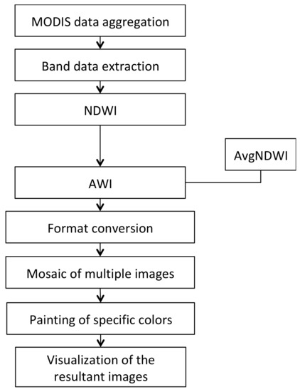
Figure 1. Flow chart of vegetation drought monitoring model.

In this section, based on the method proposed in this paper, five typical disaster-monitoring models—aerosol optical thickness inversion (AOT) model, dust storm monitoring model, and vegetation drought monitoring model, Moderate-resolution Imaging Spectroradiometer (MODIS) flood-monitoring model and synthetic aperture radar (SAR) flood-monitoring model—are implemented in this paper as use cases, as shown in Table 1. The algorithms involved in these five disaster-monitoring models are also shown in Table 1. These represent the five types of computing model, which are simple arithmetic, iterative equation, and multi-step complex calculations. Table 2 shows the computational types corresponding to these algorithms.

Table 1. Definition, algorithms, and features of five typical disaster-monitoring models mentioned in this paper.

Typical Disaster-Monitoring Models	Model Description	Algorithm Involved	Computational Complexity
Vegetation drought monitoring model	It was established based on the anomaly water index (AWI model) [43].	Band data extraction NDWI AWI AvgNDWI Mosaic Colorization Visualization Format conversion	Simple, O(n)
MODIS flood-monitoring model	Water information extracted from optical images of MODIS data using NDVI (normalized difference vegetation index) [44].	Mosaic Image segmentation Geometric correction Calibration correction NDVI Colorization Visualization Format conversion	Simple, O(n)
SAR Flood monitoring model	A neural network method for synthetic aperture radar (SAR) image segmentation and classification has been developed [45] to study flood extent extraction.	Mosaic Image segmentation Geometric correction Calibration correction Neural network classification Colorization Visualization Format conversion	Moderately complex, O(n2)
Aerosol optical thickness (AOT) inversion model	It implemented the collaborative inversion by using SYNTAM [46] algorithm.	Geometric correction Calibration correction Mosaic Colorization Visualization Image segmentation AOT	Complex, O(rn2), r is the number of iterations
Dust storm monitoring model	Extract dust information and the results will be used as mask for dust classify with brightness temperature differences.	Geometric correction Calibration correction Dust extract Bright temperature Dust intensity Dust classify Mosaic Colorization Visualization	Moderately complex, O(n2)

Table 2. The computational types of the algorithms included in the five typical disaster-monitoring models.

Number	Algorithm Type	Algorithm Name
1	Numerical calculation	NDWI, AWI, AvgNDWI, NDVI, Calibration correction, Dust extraction, Brightness temperature, Dust intensity, Colorization, Band data extraction
2	Iterative calculation	AOT
3	Statistical analysis	AvgNDWI, Dust classification, Image segmentation
4	Neighborhood operation	Mosaic, Colorization, Visualization, Format conversion, Geometric correction, Image segmentation, Neural network classification
5	Frequency domain operation	FFT

4.2. Performance Evaluation

The general model of cloud computing proposed in this paper provides an algorithm model for remote-sensing data processing on cloud computing platforms. These computing models offer excellent programmability. Three typical models were chosen for these comparative experiments. The performance comparative experiments were implemented on a desktop computer with a 4-core CPU Intel Core i5 and a cloud computing platform using 10 Hadoop nodes with Intel Xeon. Our Hadoop system consisted of 10 nodes linked by a Gigabit ethernet network, including 1 NameNode and 10 DataNodes, wherein the master node was the NameNode in addition to being a DataNode. In addition, the configuration of each node was the same, and the details are as follows: CPU characteristics were an Intel(R) Xeon(R) CPU L5640 (24 cores), 2.27 GHz; memory was 32 GB.

Real-time data processing is highlighted as one of the key features for disaster tasks processing. Using the MapReduce model not only achieve the efficiency of distributed parallel computing, but also avoid the complex process of distributed deployment. On the one hand, real-time disaster-monitoring has high requirements in the performance of data processing, and on the other hand, it also places high requirements on the programmability of the model. The MapReduce implementations offer excellent programmability. This paper adopted SLOC (source lines of code) as a quantitative indicator of programmability. Three typical disaster-monitoring models were experimented and implemented using Java language, and Table 3 shows that programming without the MapReduce model requires hundreds or thousands of lines of additional code.

Table 3. SLOC of three typical disaster-monitoring models.

Models	Programs (with MR)	Programs (without MR)
Vegetable drought monitoring model	156	782
Dust storm monitoring model	324	2754
AOT inversion model	219	2373

To compare the experimental performance, speedup was selected as the performance comparison index. The speedup defined in Equation (1) refers to the ratio of the total running time in the cloud platform to the total running time in the stand-alone environment (configured as a 4-core CPU). Total running time includes I/O time, calculation time, and system overhead.

Speedup = The total running time in the cloud platform/The total running time in the stand-alone environment

(1)

In Figure 2, it shows the speedup of the three kinds of models with the number of computing nodes ranging from 1 to 10. It can be seen that in a cloud computing environment, these models all have good performance, particularly as the number of data nodes increases. Figure 3 shows the experimental results obtained when the amount of remote-sensing data increased from 0.5 GB to about 700 GB. According to the performance curves, the vegetable drought monitoring model implemented on Hadoop exhibited excellent scalability in terms of the data volume. When implemented on a 4-core processor, the runtime metric of this model does not perform very well with increasing data amount. Although the processing power of stand-alone computing cannot be compared with the processing power of cloud computing, it could be concluded from the results, the model with MapReduce shows its excellent scalability with the increasing of data quantity.

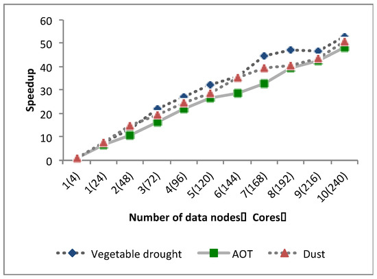
Figure 2. Speed of various models on Hadoop (1 to 10 nodes) with increasing numbers of nodes.

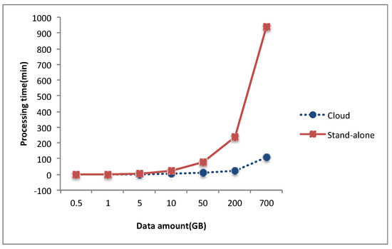
Figure 3. Runtime required to obtain the vegetable drought monitoring products versus stand-alone (4 cores) with increasing data volumes.

In addition, we also performed another performance comparison experiment using these three models. These experiments were achieved by increasing the amount of data by 2, 4, and 6 GB. Figure 4 shows the processing time of the different disaster-monitoring models due to increasing the amount of image data on the cloud computing environment.

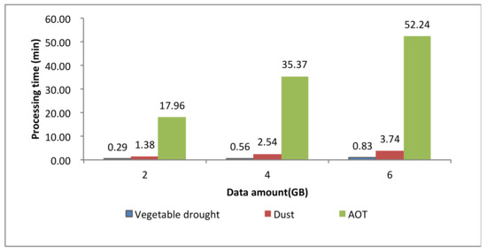
Figure 4. Processing times of various models on Hadoop with 10 nodes as the amount of data increases from 2 to 6 GB.

According to the experimental results in Figure 4, as the amount of data increased from 2 to 6 GB, the throughput of the different models was stable and slightly improved. The processing of disaster-monitoring models using cloud computing achieved excellent throughput and considerable scalability. Benefiting from the elastic resources provided by the cloud, by expanding the cluster size, the system can maintain performance levels under increased data volumes. Each disaster-monitoring model has the option to work with resources that are appropriate for its computing needs.

Each of the three models of the experiment achieved excellent performance improvements in the cloud environment, although algorithms such as iterative calculations did not reach the desired performance. The main reason may be the high computational complexity of these algorithms, i.e., the calculation amount of each task on a single machine is too large to make full use of the substantial computing power of the cloud computing architecture. Overall, most of the algorithms proposed in this paper implemented using cloud computing models achieved promising performance improvements. From the results, it can be concluded that the various algorithms implemented using the proposed cloud computing model show excellent scalability. In addition, the increase in throughput was clearly apparent, and the more data-intensive the computing, the more obvious the increase in throughput.

Therefore, the cloud computing model proposed in this paper can be used in typical disaster-monitoring applications and has good performance in terms of processing time and throughput. We conclude that the proposed cloud computing models for remote-sensing image models demonstrated their programmability and are suitable for most data-intensive disaster-monitoring algorithms.

5. Conclusions

As a new form of Internet technology service for disaster-monitoring applications, cloud computing is a highly effective method for processing data-intensive computing. Based on computational feature analysis, this paper analyzed and classified disaster-monitoring algorithms, and selected the MapReduce model to process the disaster-monitoring algorithm in the current general cloud computing model. The approach taken in this paper provides users with a simple and fast high-level abstraction of cloud computing description method, and allows users to implement the distributed design of disaster-monitoring application models and solve problems encountered in modeling, such as difficulties in programming development and code reuse.

This study implemented typical disaster-monitoring application examples based on the prototype system. This approach can be conveniently adopted by users, simplify the description and development process of disaster-monitoring applications, and verify the correctness and ease of use of the proposed method. Experiments have shown that implementing disaster-monitoring applications with MapReduce and running them into the cloud is a good solution in terms of performance and programmability. In the future, more disaster-monitoring models will be tested to verify that cloud computing is the best choice, especially for real-time processing requirements.

References

- Ma, J.; Sun, W.; Yang, G.; Zhang, D. Hydrological Analysis using Satellite Remote Sensing Big Data and CREST Model. IEEE Access 2018, 6, 9006–9016. [Google Scholar] [CrossRef]
- Jeansoulin, R. Review of Forty Years of Technological Changes in Geomatics toward the Big Data Paradigm. Int. J.Geo Inf. 2016, 5, 155. [Google Scholar] [CrossRef]
- Zhan, Q.; Yu, L. Segmentation of LiDAR Point Cloud Based on Similarity Measures in Multi- dimension Euclidean Space. Adv. Intell. Soft Comput. 2012, 141, 349–357. [Google Scholar]
- Zhang, L.; Zhang, L.; Tao, D.; Huang, X. A modified stochastic neighbor embedding for multi-feature dimension reduction of remote sensing images. ISPRS J. Photogramm. Remote Sens. 2013, 83, 30–39. [Google Scholar] [CrossRef]
- Yang, J.; Ma, Z.; Dang, J.; Wei, L.; Wang, Y. Improved fast-ica for change detection of multi temporal remote sensing images. In Proceedings of the 2018 IEEE 16th Intl Conf on Dependable, Autonomic and Secure Computing, 16th Intl Conf on Pervasive Intelligence and Computing, 4th Intl Conf on Big Data Intelligence and Computing and Cyber Science and Technology Congress(DASC/PiCom/DataCom/CyberSciTech), Athens, Greece, 12–15 August 2018; Volume 1, pp. 357–361. [Google Scholar]
- Zhang, W.; Lin, J.; Peng, J.; Lu, Q. Estimating Wenchuan Earthquake induced landslides based on remote sensing. Int. J. Remote Sens. 2010, 31, 3495–3508. [Google Scholar] [CrossRef]
- Tong, X.; Luo, X.; Liu, S.; Xie, H.; Chao, W.; Liu, S.; Jiang, Y. An approach for flood monitoring by the combined use of Landsat 8 optical imagery and COSMO-SkyMed radar imagery. ISPRS J. Photogramm. Remote Sens. 2018, 136, 144–153. [Google Scholar] [CrossRef]
- TralliT, D.M.; Blom, R.G.; Zlotnicki, V.; Donnellan, A.; Evan, D.L. Satellite remote sensing of earthquake, volcano, flood, landslide and coastal inundation hazards. ISPRS J. Photogramm. Remote Sens. 2005, 59, 185–198. [Google Scholar] [CrossRef]
- Ozelkan, E.; Chen, G.; Üstündaǧ, B. Multiscale object-based drought monitoring and comparison in rainfed and irrigated agriculture from Landsat 8 OLI imagery. Int. J. Appl. Earth Obs. Geoinf. 2016, 44, 159–170. [Google Scholar] [CrossRef]
- Ajaj, Q.; Pradhan, B.; Noori, A.; Jebur, M. Spatial monitoring of desertification extent in western Iraq using landsat images and gis. Land Degrad. Dev. 2017, 28, 2418–2431. [Google Scholar] [CrossRef]
- Cheng, T.; Li, D.; Wang, Q. On parallelizing universal Kriging interpolation based on OpenMP, Ninth International Symposium on Distributed Computing and Applications to Business. In Proceedings of the 2010 Ninth International Symposium on Distributed Computing and Applications to Business, Engineering and Science, Hong Kong, China, 10–12 August 2010. [Google Scholar]
- Maulik, U.; Sarkar, A. Efficient parallel algorithm for pixel classification in remote sensing imagery. Geoinformatica 2012, 16, 391–407. [Google Scholar] [CrossRef]
- Van Den Bergh, F.; Wessels, K.J.; Miteff, S.; Van Zyl, T.L.; Gazendam, A.D.; Bachoo, A. HiTempo: A platform for time-series analysis of remote-sensing satellite data in a high-performance computing environment. Int. J. Remote Sens. 2012, 33, 4720–4740. [Google Scholar] [CrossRef]
- Plaza, A.; Du, Q.; Chang, Y.; King, R.L. Foreword to the Special Issue on High Performance Computing in Earth Observation and Remote Sensing. IEEE J. Sel. Top. Appl. Earth Obs. Remote Sens. 2011, 4, 503–507. [Google Scholar] [CrossRef]
- Xue, Y.; Wan, W.; Ai, J. High Performance Geocomputation Developments. World SciTech R D 2008, 30, 314–319. [Google Scholar]
- Wang, P.; Wang, J.; Chen, Y.; Ni, G. Rapid processing of remote sensing images based on cloud computing. Future Gener. Comput. Syst. 2013, 29, 1963–1968. [Google Scholar] [CrossRef]
- Hu, F.; Yang, C.; Schnase, J.L.; Duffy, D.Q.; Xu, M.; Bowen, M.K.; Song, W. ClimateSpark: An in-memory distributed computing framework for big climate data analytics. Comput. Geosci. 2018, 115, 154–166. [Google Scholar] [CrossRef]
- Roy, S.; Gupta, S.; Omkar, S. Case study on: Scalability of preprocessing procedure of remote sensing in Hadoop. Comput. Sci. 2017, 108C, 1672–1681. [Google Scholar] [CrossRef]
- Zhao, Y.; Gao, J. Research on the Technological Architecture for Implementation of the Compute-intensive Spatial Information Services. Geospat. Inf. 2010, 5, 11–14. [Google Scholar]
- Xia, L.; Zhao, L.B.; Zhang, X.P.; Zhou, X.M. Study on the quality control methods of cluster-based remote sensing image processing. Int. Arch. Photogramm. Remote Sens. Spatial Inf. Sci. 2013, XL-2/W1, 31–34. [Google Scholar] [CrossRef]
- Li, G.; Liu, D. Key Technologies Research on Building a Cluster-based Parallel Computing System for Remote Sensing. LNCS 2005, 3516, 484–490. [Google Scholar]
- Kussul, N.N.; Shelestov, A.Y.; Skakun, S.V.; Li, G.; Kussul, O.M. The Wide Area Grid Testbed for Flood Monitoring Using Earth Observation Data. IEEE J. Sel. Top. Appl. Earth Obs. Remote Sens. 2012, 5, 1746–1751. [Google Scholar] [CrossRef]
- Zeng, Y.; Li, G.; Guo, L.; Huang, H. An On-Demand Approach to Build Reusable, Fast-Responding Spatial Data Services. IEEE J. Sel. Top. Appl. Earth Obs. Remote Sens. 2012, 5, 1665–1677. [Google Scholar] [CrossRef]
- Fustes, D.; Cantorna, D.; Dafonte, C.; Arcay, B.; Iglesias, A.; Manteiga, M. A cloud-integrated web platform for marine monitoring using GIS and remote sensing: Application to oil spill detection through SAR images. Future Gener. Comput. Syst. 2014, 34, 155–160. [Google Scholar] [CrossRef]
- Perez, J.F.; Swain, N.R.; Dolder, H.G.; Christensen, S.D.; Snow, A.D.; Nelson, E.J.; Jones, N.L. From global to local: Providing actionable flood forecast information in a cloud-based computing environment. J. Am. Water Resour. Assoc. 2016, 52, 965–978. [Google Scholar] [CrossRef]
- Wang, L.; Ma, Y.; Yan, J.; Chang, V.; Zomaya, A.Y. PipsCloud: High performance cloud computing for remote sensing big data management and processing. Future Gener. Comput. Syst. 2018, 78, 353–368. [Google Scholar] [CrossRef]
- Lu, W.; Wang, Y.; Jiang, J.; Liu, J.; Shen, Y.; Wei, B. Hybrid storage architecture and efficient MapReduce processing for unstructured data. Parallel Comput. 2017, 69, 63–77. [Google Scholar] [CrossRef]
- Luo, C.; He, F.; Ghezzi, C. Inferring software behavioral models with MapReduce. Sci. Comput. Program. 2017, 145, 13–36. [Google Scholar] [CrossRef]
- Zeng, X.; Garg, S.K.; Wen, Z.; Strazdins, P.; Zomaya, A.Y.; Ranjan, R. Cost efficient scheduling of MapReduce applications on public clouds. J. Comput. Sci. 2018, 26, 375–388. [Google Scholar] [CrossRef]
- Wang, W.; Ying, L. Data locality in MapReduce: A network perspective. Perform. Eval. 2016, 96, 1–11. [Google Scholar] [CrossRef]
- Lua, W.; Chen, L.; Wang, L.; Yuan, H.; Xing, W.; Yang, Y. NPIY: A novel partitioner for improving mapreduce performance. J. Vis. Lang. Comput. 2018, 46, 1–11. [Google Scholar] [CrossRef]
- Selvitopi, O.; Demirci, G.V.; Turk, A.; Aykanat, C. Locality-aware and load-balanced static task scheduling for MapReduce. Future Gener. Comput. Syst. 2019, 90, 49–61. [Google Scholar] [CrossRef]
- Gouasmi, T.; Louati, W.; Kacem, A.H. Exact and heuristic MapReduce scheduling algorithms for cloud federation. Comput. Electr. Eng. 2018, 69, 274–286. [Google Scholar] [CrossRef]
- Zou, Q.; Li, Q.; Yu, W. MapReduce functions to remote sensing distributed data processing—Global vegetation drought monitoring as example. Softw. Pract. Exp. 2018, 48, 1352–1367. [Google Scholar] [CrossRef]
- Li, Z.; Huang, Q.; Carbone, G.J.; Hu, F. A high performance query analytical framework for supporting data-intensive climate studies. Comput. Environ. Urban Syst. 2017, 62, 210–221. [Google Scholar] [CrossRef]
- Yao, X.; Mokbel, M.F.; Alarabi, L.; Eldawy, A.; Yang, J.; Yun, W.; Zhu, D. Spatial coding-based approach for partitioning big spatial data in Hadoop. Comput. Geosci. 2017, 106, 60–67. [Google Scholar] [CrossRef]
- Jing, W.; Tian, D. An improved distributed storage and query for remote sensing data. Procedia Comput. Sci. 2018, 129, 238–247. [Google Scholar] [CrossRef]
- Mazhar, M.; Rathore, U.; Ahmad, A.; Paul, A.; Wu, J. Real-time continuous feature extraction in large size satellite images. J. Syst. Archit. 2016, 64, 122–132. [Google Scholar]
- Li, X.; Song, J.; Zhang, F.; Ouyang, X.; Khan, S.U. MapReduce-based fast fuzzy c-means algorithm for large-scale underwater image segmentation. Future Gener. Comput. Syst. 2016, 65, 90–101. [Google Scholar] [CrossRef]
- Sharma, N.; Bagga, S.; Girdhar, A. Novel approach for denoising using hadoop image processing interface. Procedia Comput. Sci. 2018, 132, 1327–1350. [Google Scholar] [CrossRef]
- Xia, H.; Karimi, H.A.; Meng, L. Parallel implementation of Kaufman’s initialization for clustering large remote sensing images on clouds. Comput. Environ. Urban Syst. 2017, 61, 153–162. [Google Scholar] [CrossRef]
- Wiki Site. Available online: https://en.wikipedia.org/wiki/Neighborhood_operation (accessed on 1 January 2020).
- Bai, L.; Yan, Q.; Zhang, L. Sensitivity analysis of response of MODIS derived drought indices to drought in North China. Arid Land Geogr. 2012, 35, 708–716. [Google Scholar]
- Sai, W.; Qiuwen, Z. Method and model of water body extraction based on remote sensing data of MODIS. Comput. Digit. Eng. 2005, 33, 1–4. [Google Scholar]
- Skakun, S. A neural network approach to flood mapping using satellite imagery. Comput. Inform. 2010, 29, 1013–1024. [Google Scholar]
- Tang, J.; Xue, Y.; Yu, T.; Guan, Y. Aerosol optical thickness determination by exploiting the synergy of TERRA and AQUA MODIS. Remote Sens. Environ. 2005, 94, 327–334. [Google Scholar] [CrossRef]
© 2020 by the authors. Licensee MDPI, Basel, Switzerland. This article is an open access article distributed under the terms and conditions of the Creative Commons Attribution (CC BY) license (http://creativecommons.org/licenses/by/4.0/).