A Systematic Error Compensation Strategy Based on an Optimized Recurrent Neural Network for Collaborative Robot Dynamics

Featured Application

This research is mainly related to the simulation and control of the collaborative robot. It helps to build a more precise simulation model, design the advanced control algorithm, and achieve human-robot collaborative application with higher accuracy and more safely.

Abstract

Robot dynamics and its parameter identification are of great significance to the realization of optimal control and human–machine interaction. The objective of this research is to address the shortcomings of establishing and identifying the self-developed six-degree-of-freedom (6-DoF) collaborative robot dynamics, which leads to a large error in the predicted torque of the proposed robot. A long short-term memory (LSTM) in an optimized recurrent neural network (RNN) is proposed to compensate the dynamic model of the proposed 6-DoF collaborative robot based on the consideration of gravity, Coriolis force, inertial force, and friction force. The analysis and experimental findings provide promising results. The compensated collaborative robot dynamic model based on LSTM in an optimized RNN displays a good prediction on the actual torque, and the root-mean-square (RMS) error between predicted and actual torques are reduced by 61.8% to 78.9% compared to the traditional dynamic model. Results of the experimental applications demonstrate the validity of the proposed systematic error compensation strategy.

1. Introduction

An accurate robot dynamic model can be used as the basis for building simulation models, verifying advanced control algorithms, and performing in-depth analysis of control systems [1]. With the rising requirements of dynamic performance and the concept of collaborative robots, conventional model-free control methods, such as the proportion integral differential (PID) control, not only exhibit low trajectory tracking accuracy and poor anti-disturbance capabilities, but also present difficulty in implementing human–robot interaction tasks, such as collision detection and compliance control [2].

For dynamic models of multi-axis serial chain robots, gravity, Coriolis force, inertial force and friction are generally considered. However, the reducer flexibility, inertia force of motor rotors, etc. are rarely taken into consideration. In addition, a precise dynamic model of the robot manipulator relies heavily on an accurate friction model [3]. Accurate friction models cause some error between the calculated torque and the actual torque, which hinders the good realization of collision detection, lead-through programming, and compliance control. Many researchers have proposed different error compensation policies [4,5]. Machine learning methods, such as back propagation (BP) neural network [6] and radial basis function (RBF) network [7,8], are also used to fix or compensate errors. C Li et al. [9] present a novel dynamic modeling method by using a recurrent neural network (RNN) with an incomplete state system variables observation. The RNN family are also used for robotic manipulator model learning tasks [10] and approximating robot dynamical models [11,12]. However, studies with many kinds of complex characteristics combined are limited.

As for parameter identification, there is the disassembly measurement calculation method [13], the disassembly experiment measurement method [14], the non-disassembly experiment measurement method [15], and theoretical identification [16], etc. The disassembly method cannot, or has difficulty in, calculating the characteristics of robot joints [17]. The inertial tensor matrix obtained by the theoretical identification method may not necessarily be positive or definite under any form or situation. It is impossible to exist in practice, and its control is unstable [18].

To this end, an optimized RNN is proposed to compensate the error of the collaborative robot dynamic model, and the pipeline is as follows. First, the dynamic equations are established, and then the non-disassembly experimental measurement combined with the least square method is used to identify the parameters. Next, in order to tackle unmodeled characteristics or the inaccurate modeling of collaborative robots, an optimized RNN is put forward. With this method, the errors of the dynamic model are reduced, and accuracy of torque prediction is improved. In the final experiment, a motor current is used to evaluate the joint torque instead of mounting expensive and inconvenient torque sensors to fulfill the verification of the compensation method.

This paper is organized as follows: Section 2 presents the dynamic model of the self-developed six-degree-of-freedom (6-DOF) collaborative robot; Section 3 shows the excitation trajectory generation; Section 4 presents the error compensation by an optimized recurrent neural network; Section 5 shows the results of the experiment using a self-developed 6-DOF collaborative robot; Section 6 concludes the paper.

2. Dynamic Model of Collaborative Robot

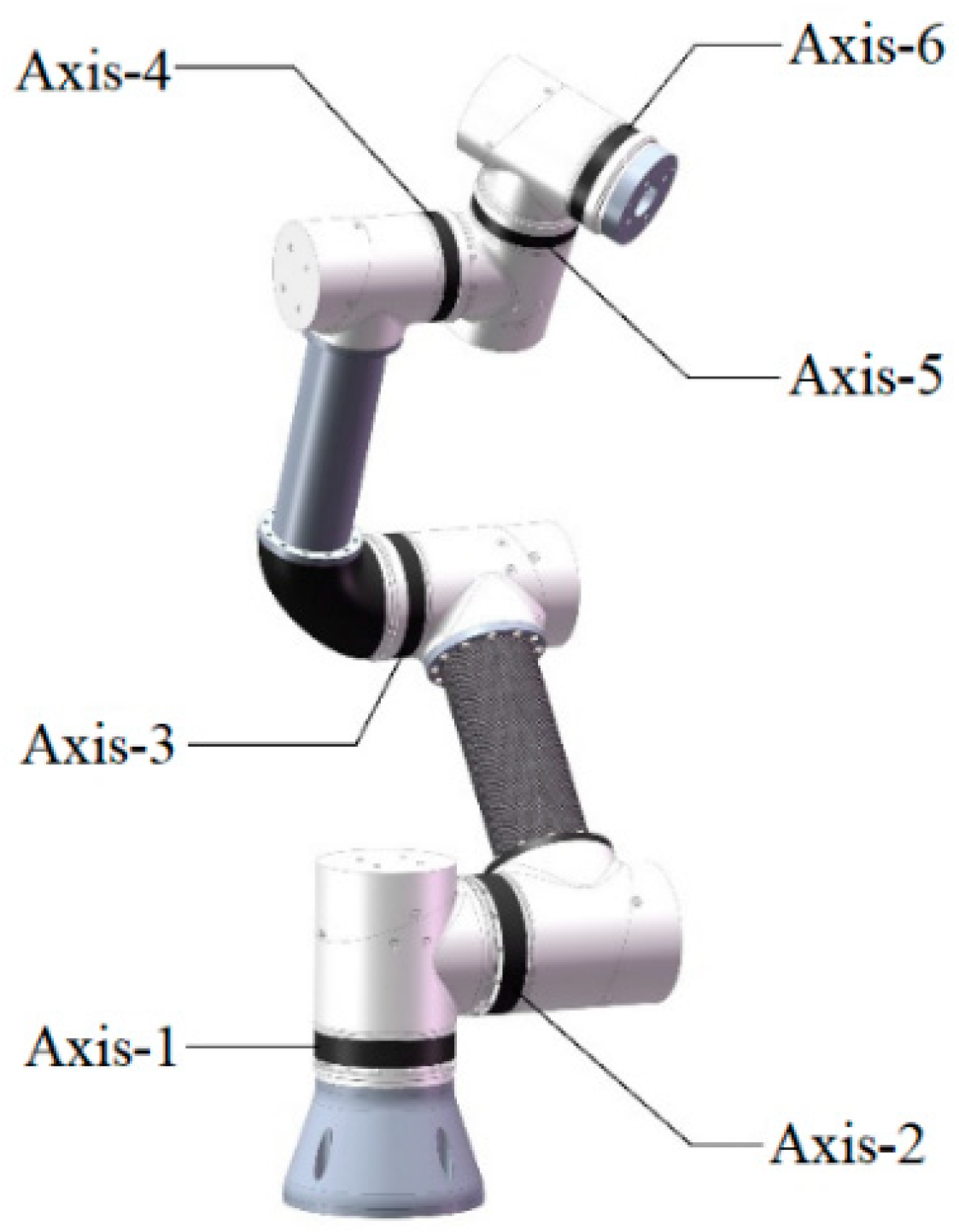
The 3D model and Denavit-Hartenberg (D-H) diagram of the proposed collaborative robot are presented in Figure 1 and Figure 2, respectively. Note that the 2nd, 3rd, and 4th joint of the collaborative robot are parallel to each other, which proves the existence of a closed-form solution for inverse kinematics. Considering gravity, Coriolis force, inertial force and friction, the dynamic equation is derived by the Euler–Lagrangian method, and the driving torques of robot joint can be expressed as:

$$\mathbf{\tau }=M\left(q\right) \ddot{q} + H\left(q,\dot{q}\right)+G\left(q\right)+{\mathbf{\tau }}_{\mathit{f}}$$

(1)

where $q$, $\dot{q}$ and $\ddot{q}$ are the joint position vector, joint velocity vector and the joint acceleration vector, respectively; M(q) is the inertial matrix of the manipulator; $H\left(q,\dot{q}\right)$ is the centrifugal force and Coriolis force matrix; G(q) is the gravity matrix; ${\mathbf{\tau }}_{\mathit{f}}$ is the friction force vector.

The friction mainly caused by the joint reducer and bearing is not negligible [18], which leads to a relatively large error in the calculated torque, especially when the velocity changes its direction; that is, near the zero-point of speed. Therefore, the Stribeck friction model is introduced, and the equation is simplified as below:

$${\mathbf{\tau }}_{\mathit{f}}=D\dot{q}+\mu \mathrm{sgn}\left(\dot{q}\right)$$

(2)

where D is the viscous friction coefficient vector and μ is the Coulomb friction coefficient.

According to Equations (1) and (2), Equation (3) can be obtained:

$$\mathbf{\tau }=M\left(q\right) \ddot{q}+H\left(q,\dot{q}\right)+G\left(q\right)+D\dot{q}+\mu \mathrm{sgn}\left(\dot{q}\right)$$

(3)

Equation (1) can be written in the following linear form:

$${\mathbf{\tau }}_{\mathit{r}}=\Phi \left(q,\dot{q},\ddot{q}\right)\mathbf{\theta }+{\mathbf{\tau }}_{\mathit{f}}$$

(4)

where $\Phi \left(q,\dot{q},\ddot{q}\right)$ is the observation matrix, which is only related to the joint position, velocity, acceleration, and the structure of the robot. θ is the basic inertial parameter vector, including mass, centroid and moment of inertia.

Due to the structure and installation of the collaborative robot, some elements in θ are redundant to the dynamic model and do not contribute to the joint torque when the collaborative robot is working, and so cannot be identified through experiment. Additionally, some elements are linearly related, and cannot be identified individually. Therefore, the parameters must be reorganized in order to obtain a minimum set of identification parameters, also known as the minimum inertial parameter set. Equation (3) should therefore be rewritten as:

$${\mathbf{\tau }}_{\mathit{r}}=\Phi \left(q,\dot{q},\ddot{q}\right){\mathbf{\theta }}_{\mathit{r}}+{\mathbf{\tau }}_{\mathit{f}}$$

(5)

where ${\mathbf{\tau }}_{\mathit{r}}$ is the reconstructed observation matrix, ${\mathbf{\theta }}_{\mathit{r}}$ is the minimum inertia parameter set vector.

Regarding the accuracy of the dynamic model and the compensation method for collaborative robots, the root-mean-square (RMS) error of the predicted torque (calculated torque) relative to the actual measured torque is used in order to evaluate this. Smaller RMS errors mean better dynamic models and compensation methods, otherwise they need to be improved.

3. Excitation Trajectory Generation

The measurement method of the non-disassembly experiment needs to drive the robot to obtain the required data. Considering the calculation accuracy and the experimental feasibility, the collaborative robot trajectory, especially the excitation trajectory, must fulfill various conditions, such as maximum moving range, speed, and the acceleration of each joint.

A six-axis robot has a highly complex dynamics calculation, and thus needs to be simplified. The identification of the dynamic parameters for each joint can be done individually, that is, when identifying the dynamic parameters of the last three joints, the other three joints can be locked. As a result, the difficulty of identification is greatly reduced and more targeted. The analysis, calculation, and experimental procedure of the first three joints is the same as the last three joints and can be done separately. Limited to this research process, this paper only focuses upon the dynamic parameters of the typical last three joints of the collaborative robot.

In the experiment, the first five terms of the Fourier series, namely Formula (6), are used as the excitation trajectory. Because it is a periodic function, it is convenient to repeat this experiment as many times as needed.

$$q_i\left(t\right)=q_{i,0}+{\displaystyle \sum }_k^5\left(a_{i,k}\sin \left(k{\omega }_{f}t\right)+b_{i,k}\cos \left(k{\omega }_{f}t\right)\right)$$

(6)

where $q_i\left(t\right)$ is the ith joint trajectory function of time t, ${\omega }_f$ is the fundamental frequency, $q_{i,0}$ is a constant offset. Each trajectory contains 11 parameters, namely $q_{i,0}$, $a_{i,k}$, $b_{i,k}$, and ${\omega }_f$ = 1 (i = 1, 2, 3, 4, 5).

The quality of the excitation trajectory is closely related to the ability of the observation matrix to suppress noise and morbidity, which directly affects the accuracy of the identification parameters. Here, the objective function is defined as the condition number of the observation matrix W:

$$J=\mathrm{Cond}\left(\mathit{W}\right)$$

(7)

where $\mathrm{Cond}\left(\mathit{W}\right)={\sigma }_{\mathit{max}}\left(\mathit{W}\right)/{\sigma }_{\mathit{min}}\left(\mathit{W}\right)$, ${\sigma }_{max}\left(\mathit{W}\right)$ and ${\sigma }_{min}\left(\mathit{W}\right)$ are the maximum and minimum singular value of W, respectively.

The smaller the value of the objective function, the lower the sensitivity of the identification parameters to the measurement error is, and the higher the accuracy of parameters identification achieved by the experiment can be. Meanwhile, it is also necessary to consider the limitations of the actual robot performance. If the moving range, velocity, acceleration, and the status of start and stop points are taken as constraints, the optimization problem of the excitation trajectory can be described as:

$$\{\begin{array}{c}\min \left(J\right)\\ q_{min}\le \left|q_i\right(t\left)\right|\le q_{max}& \forall i,t\left(a\right)\\ {\dot{q}}_{min}\le \left|{\dot{q}}_l\right(t\left)\right|\le {\dot{q}}_{max}& \forall i,t\left(b\right)\\ {\ddot{q}}_{min}\le \left|{\dot{q}}_l\right(t\left)\right|\le {\ddot{q}}_{max}& \forall i,t\left(c\right)\\ q_i\left(t_0\right)=q_i\left(t_M\right)=0& \forall i,t\left(d\right)\\ {\dot{q}}_l\left(t_0\right)={\dot{q}}_l\left(t_M\right)=0& \forall i,t\left(e\right)\\ {\ddot{q}}_l\left(t_0\right)={\ddot{q}}_l\left(t_M\right)=0& \forall i,t\left(f\right)\end{array}$$

(8)

where $q_{min}$, ${\dot{q}}_{min}$, ${\ddot{q}}_{min}$, $q_{max}$, ${\dot{q}}_{max}$, ${\ddot{q}}_{max}$ are the boundary values of angle, speed and acceleration of each joint, respectively. $t_0$, $t_M$ are the start and end times of each period, respectively. Since the excitation trajectories are Fourier series, both periodicity and continuity are ensured, and the constraints at the end time $t_M$ can also be omitted from the actual optimization calculation.

Equation (8) is a nonlinear, multi-constrained optimization problem, which can be optimized using NSGA and other target optimization algorithms [19]. The optimized excitation trajectory is shown in Figure 3. As evident in Figure 3, the shift of the 4th, the 5th, and the 6th joint smoothly change with time. The start and end points of the curves are all zero, and the amplitude is relatively large, but does not exceed the limitation. This optimized trajectory will be used for the experiments in Section 5.

When it comes to the test set, a different excitation trajectory can be generated by adding a new constraint based on Equation (6). To apply a new constraint $q_i\left(t=3.8\right)=0$, the test set trajectory is shown in Figure 4.

As detailed in Figure 4, the curve of the test set data is smooth and continuous, and there is enough difference compared to the training set shown in Figure 3. The generalization ability of the network can be tested while making full use of the collaborative robot performance. The zero-point set at t = 3.8 s can be used to check the zero-point error during the experiment, and could help to monitor the working state of the collaborative robot.

In the subsequent experiment stage, the robot will follow the trajectory presented in Figure 3 and Figure 4. When the robot is moving, a controller collects the actual position, velocity, and acceleration. These data generate the training set $F_{tr}$ and the test set $F_{te}$. Each of the data sets contain calculated torque (predicted torque), actual torque, and the actual position of every joint at each moment. The predicted torque is calculated using Equation (5).

4. Error Compensation by RNN

RNN is a set of neural networks used to process sequence data, and the long short-term memory (LSTM) unit network is used to solve the problems of long-term dependency and gradient explosion/disappearance in the early-time RNN. LSTM has made great progress in the preservation of historical information and in the prediction of future information [20]. This study will further explore the application of LSTM in collaborative robot dynamics.

The kinematic and dynamic data of collaborative robots represent continuous series in time. Some errors, such as the memory effect of friction and the time-varying characteristics of motor parameters caused by temperature changing, are very suitable to be compensated by LSTM networks. In this study, LSTM cell units with cell state and gate structure are used to achieve a better compensation effect.

The detail of an LSTM cell unit is shown in Figure 5, which adds a cell state vector C and related gate structure. It can better solve the problem of gradient explosion and gradient disappearance in ordinary RNN cells by controlling forgetting and memory. The forward calculation process is:

$$\{\begin{array}{c}{f}_t=\sigma \left(W_f·\left[h_{t-1},x_t\right]+b_f\right)\\ i_t=\sigma \left(W_i·\left[h_{t-1},x_t\right]+b_i\right)\\ {\tilde{C}}_t=\tanh \left(W_C·\left[h_{t-1},x_t\right]+b_C\right)\\ C_t=f_t\ast C_{t-1}+i_t\ast {\tilde{C}}_t\\ o_t=\sigma \left(W_o\left[h_{t-1},x_t\right]+b_o\right)\\ h_t=o_t\ast \tanh \left(C_t\right)\end{array}$$

(9)

The training method of an LSTM network is Back Propagation Through Time (BPTT), which is similar to BP algorithm, including the steps of forward calculation, reverse calculation, computing gradient, and updating parameters.

There are many types of gradient-based optimization algorithms. In this paper, the Adaptive Momentum Estimation (Adam) algorithm is adopted [21]. This algorithm is an effective gradient-based stochastic optimization method, which can calculate adaptive learning rates for different parameters, and takes up less storage resources. Compared with other stochastic optimization methods, the Adam algorithm performs better in most practical applications [22].

A pipeline of LSTM network-based collaborative robot dynamic compensation is depicted in Figure 6. As detailed in Figure 6, this pipeline includes LSTM network, data set generation, and network training methods. The input and output layers of the LSTM network are fully connected networks, and the hidden layer consists of LSTM cell units. The main steps are:

(1)

Collect raw data (position, velocity, acceleration, torque);

(2)

Raw data are used by the dynamic model to predict the torque, i.e., the uncompensated predicted torque;

(3)

The original data of both training set and test set are normalized, including uncompensated predicted torque, actual torque and actual position;

(4)

The training set feeds into the fully connected input layer;

(5)

Iterative calculation in the hidden layer;

(6)

Output layer gives the predicted torque after LSTM compensation, i.e., the compensated predicted torque;

(7)

The loss is RMS error of the compensated predicted torque relative to the actual measured torque;

(8)

Optimize the network parameters by Adam optimizer;

(9)

Apply the updated weight;

(10)

The test set calculates the compensated predicted torque through the network and evaluates the compensation effect.

The LSTM network is implemented based on Tensorflow 1.15.0, an open source machine learning platform. According to experience and actual conditions, hyper-parameters of the network are listed in

Table 1. Hyper-Parameters of LSTM Network.

Parameters	Value
Time step	100
Batch size	50
Input size	9
Output size	3
Cell size	64
Total Layer	3
Learning rate	0.05

.

The input vector includes calculated torque, actual torque and the actual position of the 4th, 5th, and 6th joint at each moment. The output vector includes the predicted moments of the next moment of the 4th, 5th, and 6th joint. The cell size of the network is selected according to the amount of system characteristics and data. The loss function is the RMS error of the predicted torque relative to the actual torque at each moment, namely:

$$\mathrm{Loss}=\sqrt{\frac{1}{N}{{\displaystyle \sum }}_{i=1}^N{({\widehat{\tau }}^{\left(i\right)}-{\tau }^i)}^2}$$

(10)

where N is the number of samples in the data set, namely the number of sampling points for the continuous movement of the robot; ${\widehat{\tau }}^{\left(i\right)}$ is the predicted torque value; ${\tau }^{\left(i\right)}$ is the actual torque.

5. Experimental Procedures

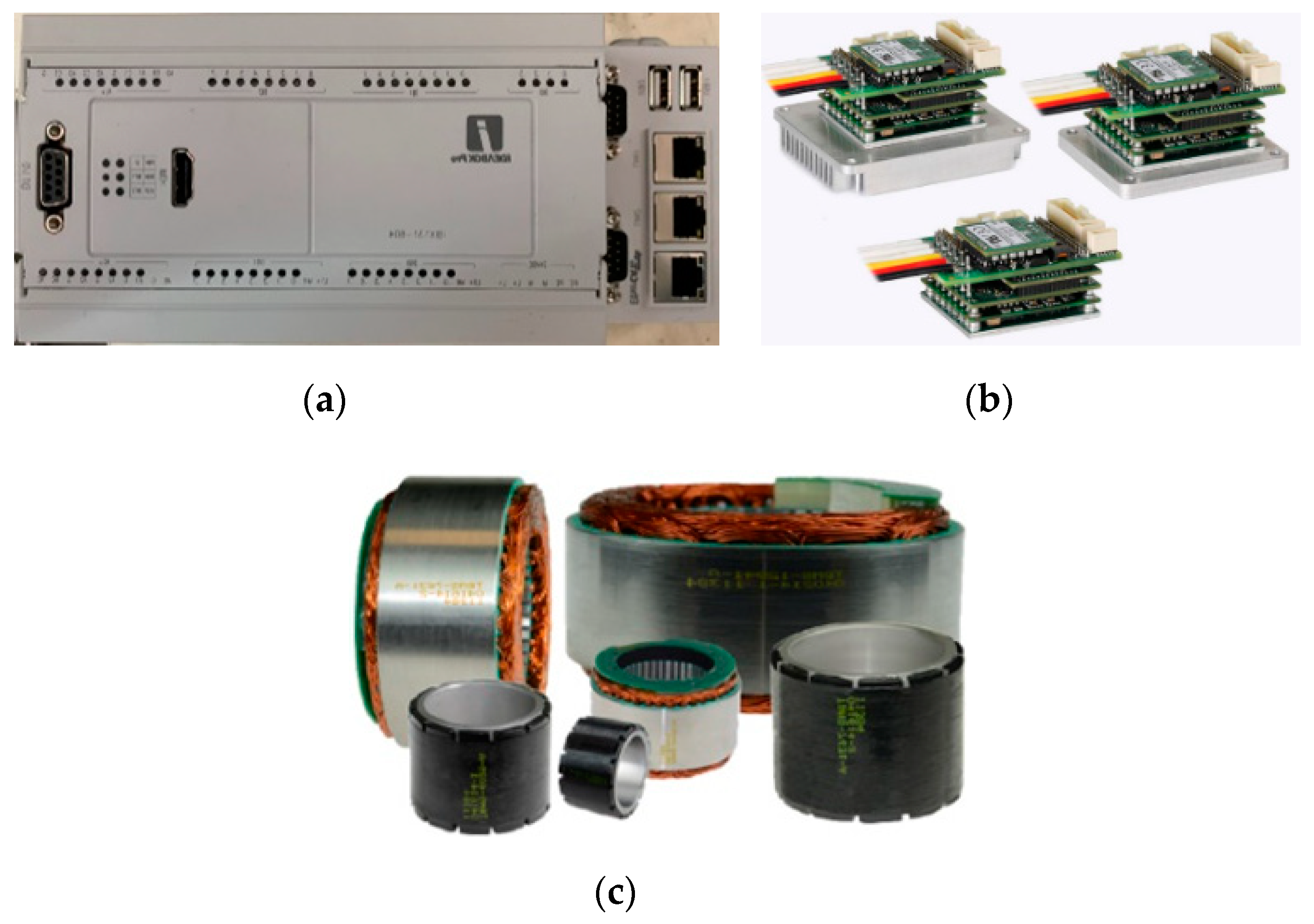
Experimental analyses have been carried out with a self-developed 6-DOF collaborative robot under actual testing conditions. Figure 7 reveals the prototype of the proposed collaborative robot, and some of the key parts are compared in Figure 8. As evident in Figure 7 and Figure 8, the collaborative robot joints are mainly composed of a harmonic drive, a frameless motor, and a motor driver. The robot controller is Softlink(R) iDEABOX Pro and the motor driver is Elmo(R) Twitter, which both support EtherCAT to allow high speed low latency communication with each other.

Only the typical 4th, 5th, and 6th joint of the collaborative robot are tested and analyzed in this experiment. Since the last three linkages are light and short, gravity and inertia are relatively small. Accordingly, the unmodeled or inaccurately modeled factors such as friction and inertia of the motor rotor will lead to greater relative errors. Therefore, the proposed error compensation technology provides great practical application value.

Servo drivers are set to the cyclic synchronous position mode. Servo drivers and the robot controller are communicated through EtherCAT, and the controller sends serial points of the excitation trajectories in Figure 3 and Figure 4 to the driver at a fixed frequency of 100 Hz, in order to ensure continuous and smooth movement. While the robot is moving, the controller also communicates with the driver to collect data such as position, velocity and current. Note that only the dynamics of the last three joints are studied, and the position commands of the 1st joint to the 3rd joint are always kept at zero.

Because the control method does not affect the intrinsic characteristics of the robot, the control algorithm adopted in this experiment is the common three-loop structure for servo motor. The three loops include the current loop, the velocity loop and the position loop from inner layer to outer layer, respectively. All three control loops are PID controller with feedforward signals. The overall control scheme with EtherCAT index indicator of each motor is shown in Figure 9.

The data are collected by driving the collaborative robot moving as the excitation trajectory. The training set $F_{tr}$ and the test set $F_{te}$ are obtained from the excitation trajectory, and are presented in Figure 3 and Figure 4, respectively.

The excitation trajectory above and the experimental data are used as the training data for LSTM network. RMS errors of the theoretically calculated torque and the actual torque are used as the loss function. As the LSTM network training epoch increases, the loss gradually decreases, as shown in Figure 10.

Figure 11 presents the actual motor current of axis 4, 5 and 6, and to avoid unexpected noise, the raw data are processed by Kalman filter. Figure 12 and Figure 13 compare the actual torque, predicted torque, and error of axis 5 before and after compensation under the excitation trajectory of the test set, respectively. RMS errors of the predicted torque relative to the actual torque before and after the compensation of each joint are listed in

Table 2. RMS Error of Calculated Torque between Real Value.

Joint	Uncompensated/N·m	Compensated/N·m
4	3.61	1.21
5	4.84	1.02
6	6.10	2.33

. As can be seen from the figures and table, compared to the uncompensated model, the RMS errors of the predicted torque via theoretical calculation and the actual torque of the 4th to the 6th joints are reduced by 66.5%, 78.9% and 61.8%, respectively. Experimental procedures show promising results, in that the errors of the dynamic model after LSTM network compensation displays a significant decrease in torque prediction compared with the uncompensated model.

6. Conclusions

The proposed self-developed 6-DOF collaborative robot in this paper is provided with a light structure, small inertia force, and gravity. However, the unmodeled or inaccurately modeled factors, such as friction force and rotor inertia force, could result in the modeling inaccuracy of a traditional dynamic model, and a large error in the calculation of predicted torque relying on the general dynamic equation. In order to solve the error compensation of the dynamic model of the proposed collaborative robot, a systematic error compensation method based on an optimized LSTM network in an optimized RNN is used to compensate the error of the predicted torque relative to the actual torque.

Experimental results show that the RMS errors of predicted torque relative to actual torque of the 4th, 5th, and 6th joints have decreased by 66.5% to 78.9% compared with the uncompensated model, and thus the effect is remarkable. Therefore, it is suggested that the proposed error compensation technology based on LSTM network is feasible and effective, and provides a good foundation for future dynamic control research.