Deep Learning Models Compression for Agricultural Plants

Abstract

Deep learning has been successfully showing promising results in plant disease detection, fruit counting, yield estimation, and gaining an increasing interest in agriculture. Deep learning models are generally based on several millions of parameters that generate exceptionally large weight matrices. The latter requires large memory and computational power for training, testing, and deploying. Unfortunately, these requirements make it difficult to deploy on low-cost devices with limited resources that are present at the fieldwork. In addition, the lack or the bad quality of connectivity in farms does not allow remote computation. An approach that has been used to save memory and speed up the processing is to compress the models. In this work, we tackle the challenges related to the resource limitation by compressing some state-of-the-art models very often used in image classification. For this we apply model pruning and quantization to LeNet5, VGG16, and AlexNet. Original and compressed models were applied to the benchmark of plant seedling classification (V2 Plant Seedlings Dataset) and Flavia database. Results reveal that it is possible to compress the size of these models by a factor of 38 and to reduce the FLOPs of VGG16 by a factor of 99 without considerable loss of accuracy.

1. Introduction

Deep learning (DL) is playing a crucial role in precision agriculture to improve the yield of the farm [1,2,3]. However, applying deep learning in agriculture involves the acquisition and processing of a large amount of data related to crop. These data are essentially collected, based on wireless sensors (aboveground or underground), drones, satellites, robots, etc. Due to the huge amount of parameters, DL models are usually inefficient on low-cost devices with limited resources [4]. As a result, they are usually deployed on remote servers. Remote processing raises two issues: the latency of the network, and the bandwidth saving. Farm automation solutions such as automatic harvesting [5], fruit counting [6], etc., require a very short response time that is not easily provided by remote computation. The closer the processing unit is in the farm, the smaller is the latency. Apart from latency, most weakly industrialized economies experience low Internet penetration rates, especially in rural areas where agricultural activities are mainly performed. Many rural areas that do have connectivity have low bandwidths that only allow limited data traffic [7,8]. This can also increase the response time since DL models process a huge amount of data. A recent approach to overcome those limitations is infield deployment that can provide more efficient real-time reaction, critical for crop monitoring. Infield deployment generally relies on edge computing [9] that allows incoming data to be analyzed close to the source with a minimal footprint.

Edge computing adapts well to limited computing performance and it is suitable for infield inference, which enables real-time reaction and facilitates the sending of refined data or results over narrowband networks. Since devices used in agricultural field are resource-limited, using infield DL models is considered to be a significant challenge.

Few works [10,11] on DL in agriculture take into account the limitation of resources. Authors designed a model compression technique based on separable convolution and singular value decomposition. They applied their technique on very deep convolutional neural networks (CNNs) for plant image segmentation, with the aim of deploying the new model infield.

In contrast to the works of [10,11], which focus on segmentation (background/flower), this paper focuses on classification, which is a more common task in the application of DL in agriculture. This work proposes a combination of two methods namely pruning and quantization, which are applicable to any type of neural network and allows to obtain higher compression ratio. Three DL models (LeNet5, VGG16, and AlexNet) are compressed and applied on two datasets used in agriculture: V2 Plant Seedlings Dataset [12] and Flavia database [13].

The rest of the paper is organized as follows: Section 2 briefly presents common DL models as well as the constraints of deploying such models on low-cost and limited-resource devices. Section 3 describes of up-to-date techniques in model compression. The proposed model approach and experimental setup are discussed, respectively, in Section 4 and Section 5. The evaluation on plant disease datasets is done in Section 6, and Section 7 concludes the present work.

2. Deep Learning Models

Several DL models have been proposed in the literature. This section presents common models that usually serve as a basis to other models, and the constraints of deploying DL models on low resource devices.

2.1. State-of-the-Art Models

The first major success of CNNs in the task of pattern recognition dates back to LeNet (LeNet5) [14]. It was designed for handwritten and machine-printed character recognition. According to current trends, LeNet5 is a very simple model. The network architecture encompasses two sets of convolutional and average pooling layers. Those layers are followed by a flattening layer, then two fully connected layers and finally a softmax classifier.

AlexNet [15] follows the ideas of LeNet5, incorporating several new concepts and more depth. It consists of eight layers: five convolutional layers and three fully connected (FC) layers. The great success of AlexNet is due to several advantages such as the ReLU activation function, the dropout, the data augmentation, as well as the use of GPUs to speed up computation.

Later VGGNet [16] based on AlexNet has been developed as an enhancement that replaces large convolutional filters of size 11 × 11 and 5 × 5, respectively, in the first and second convolutional layer in AlexNet with multiple small filters of size 3 × 3. With a given receptive field (the effective area size of input image on which output depends), several smaller filters stacked together are better than one larger filter because several nonlinear layers increase the depth of the network, allowing it to learn more complex features at a lower cost.

Another important model is ResNet [17]. The fundamental breakthrough of ResNet was to enable the training of extremely deep neural networks with more than 150 layers with no loss in gradient. Before training with residual layers, very deep neural networks were difficult to train because of vanishing gradients problem. ResNet introduced the concept of jump connection (residual connection) which allows the model to learn an identity function that ensures that upper layers will work at least as well as lower layers.

In the trend of developing DL models, Google has proposed Inception GoogleNet or Inception [18]. It is essentially a CNN that has 27 layers depth. In CNNs, much of the work consists of choosing the right layer to apply with the most common options (filters sizes, types of pooling, etc.). It is sufficient to find the optimal local construction and repeat it spatially. GoogleNet uses all these layers in parallel and then combines their results.

These models are very often reused for different tasks in agriculture. Table 1 shows some important works that use state-of-the-art models in agriculture.

Table 1. Some work using state-of-the-art models in agriculture.

Tasks	Models Used	Reference
Plant recognition	AlexNet	[21,22]
Plant disease detection	AlexNet and Inception	[23]
Tomato fruit counting	Inception-ResNet	[6]
Plant species classification	VGG16	[24]
Mixed crops semantic segmentation	VGG16	[25]
Obstacles detection in the farm	VGG16 and AlexNet	[26]
Fruit detection	Faster R-CNN and VGG16	[27,28]
Mango fruit detection and yield estimation	Faster R-CNN	[29]
Plant disease recognition	CaffeNet	[30]

2.2. Deep Learning Models Constraints

Typically, these deep learning models are trained and deployed on GPUs because of their computing power requirements. Infield training and/or deployment of such models in low-cost equipment are therefore subject to some main constraints: the memory, the computing power, and the energy.

Memory: The most obvious bottleneck for DL is the working memory, but also the storage space, especially when working with low resource devices. Models commonly require storage space in the order of hundreds of MB due to their complex representation, far above 32 MB offered by IMote 2.0 or 64 MB proposed by Arduino Yun [19]. From a practical point of view, this inflates sensor apps dramatically and usually dwarfs application logic [20]. Concerning the runtime requirements, the required working memory at peak time will often preclude a particular platform from using a model even if this platform has the necessary storage space to hold the model representation. It is not uncommon for a single model layer to require tens or hundreds of MBs and this might be 90% more than the average layer consumption within the model. In such cases, manual customization of the model is necessary before it runs completely up to the final layer.

Computing power: Models such as VGGNet, even when carefully implemented on embedded platforms, have proven to take a couple of minutes for a single image due to the paging required to overcome a large memory footprint [20]. Likewise, despite their high computing power, devices such as smartphones present challenges in running deep models with latency tailored to user interaction. This typically leads to the use of models that offload their computation to the cloud, or at least to a GPU. Computational requirements are also strongly dependent on the architecture of the model, with some layers such as convolutional layers being much more related to computation than feed-forward layers (which are more related to memory). As a result, simple architecture changes can have a significant impact on the running time.

Energy: Related to computation, the power consumption of deep models due to the excessive running time for a single inference can be very expensive for equipment used in continuous monitoring. In addition, the access to a power source in remote areas such as farms is not always guaranteed. That is why equipment are usually battery powered. The limited energy of battery therefore requires the minimization of the power consumption of deep learning models.

To overcome present challenges and to allow the deployment of DL models on resource limited equipment require the compression of models.

3. Related Works on Models Compression

The idea of compressing models has originated from the observation that many of the parameters used in deep neural networks (DNNs) are redundant [31] and thus may be removed without loss of performance. In addition, using a very deep model (in terms of number of layers) is not always necessary, and it may be possible to eliminate some of the hidden layers without considerably decreasing the accuracy [32]. As a consequence of the compression, the complexity will be reduced [9], which makes the application suitable for low resources.

3.1. Parameter Pruning

In many neural networks, a large number of parameters do not contribute significantly to the network’s predictions [33]. Pruning is a simple but efficient method to introduce sparsity in deep neural networks. The idea of parameters pruning consists of reducing the size of the model by removing the unnecessary connection from the neural network. Pruning contributes to decrease the computation cost along with the storage and memory, while keeping an acceptable performance. Several heuristics have been studied to select and delete irrelevant connections.

3.1.1. Pruning Schedule

Pruning schedule is divided into two categories: one shot pruning and iterative pruning. One shot pruning aims to achieve the desired compression ratio in a single step. More aggressive than iterative pruning, redundant connections are pruned once with respect to the saliency criterion and the sparse pruned network is retrained. The main advantage is that it does not require additional hyper-parameters or pruning schedule. The authors of [34] propose a data-dependent selective pruning of redundant connections prior to training. For this purpose, the importance of the connections is evaluated by measuring its effect on the loss function.

In contrast to one shoot pruning, iterative pruning consists of gradually removing connections until obtaining the targeted compression ratio. As the configuration of the model changed, it has to be retrained to readapt the parameters after pruning iterations to recover the accuracy drop [35].

3.1.2. Salience Criteria

Brain Damage [36] and Optimal Brain Surgeon [37] used the second-order Taylor expansion to calculate the parameters’ importance. It consists of removing parameters with the least increase of error approximated by second order derivatives. However, in very deep networks, computing the Hessian or Hessian inverse over all the parameters can be too expensive. A simpler method consists of using the magnitude of weight value.

Let us consider $\mathit{W}$ the set of weight tensors and $w_{ij} ϵ \mathit{W}$, the magnitude-based connections pruning supposes removing all connections whose weight absolute value is lower than a certain threshold $T$, as given in Equation (1).

$$w_{ij}=\{\begin{array}{c}0 if w_{ij}<T\\ w_{ij} otherwise\end{array}$$

(1)

An intuitive constraint for non-zero connections selection consists of weights regulation. Using the $L_1$ and $L_2$ norms, Song Han [33] reduced the number of parameters of AlexNet and VGG-16 by factors of 9 and 13, respectively. Some other methods learn pruning criteria using reinforcement learning (RL) [38,39]. RL based pruning focuses on learning the proper pruning criteria for different layers via the differential sampler.

3.1.3. Granulation

Depending on the structure, pruning can be classified in two main categories: unstructured pruning and structured pruning. The unstructured pruning approach, also called fine-grained, removes individual weights unconstrained from the local structure. However, pruning can remove entire structures (kernel, filter, etc.). Figure 1 illustrates the different level of granularity neural network pruning.

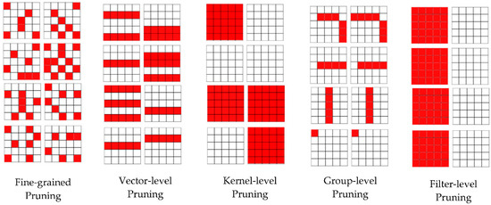
Figure 1. Neural network pruning granularity.

Fine-grained pruning methods remove network parameters independently to the data structure. Any unimportant parameters in the convolutional kernels can be pruned. This consists of using salience criteria to rank individual weights then remove the less important. Recently the authors of [33] proposed a deep compression framework to compress deep neural networks in three steps: pruning, quantization, and Huffman encoding. By using this method, AlexNet could be compressed by a factor of 35 without drops in accuracy. The work uses a polynomial decay function to control the step sparsity level. High sparsity levels can be achieved, so the model can be compressed to require less memory space and bandwidth. However, a poor pruning can lead to a drop in accuracy. In addition, these approaches result in unstructured parsimony of the model. Without specialized parallelization techniques and hardware that can perform computations on sparse tensors, this does not accelerate the computation. Another strategy is to remove entire data structures, such as kernels or filters.

Vector-level pruning methods prune 1D vectors in the convolutional kernels, and kernel-level pruning methods prune 2D kernels in the filters. Like fine-grained pruning, vector-level pruning and kernel-level convert dense connectivity into sparse connectivity, but in a structured way [40].

Group-level pruning tries to eliminate network parameters according to the same sparse pattern on the filters [41]. In this way, convolutional computation can be efficiently implemented with reduced matrix multiplication. In [42], the authors propose a group-wise convolutional kernel pruning approach inspired by optimal brain damage [36]. The authors of [35] used group Lasso to learn a sparse structure of neural networks.

Filter-level pruning reduces convolutional layers size by removing unimportant filters. This leads to a simplification of the network architecture. Layer filters are removed, and also the size of the output features-map is reduced and directly impacts on the convolutional layers’ speedup. Pruning filters with low absolute weights sum is similar to pruning low magnitude weights. Filter-level pruning maintains dense tensors which leads to a lower compression ratio but is more efficient for accelerating the model with less convolution operation. The authors of [43] proposed ThiNet, a filter-level pruning framework to simultaneously accelerate and compress convolutional neural networks. They used the next layer’s feature map to guide the filter pruning in the current layer.

Unstructured sparsity produces very high compression rates but allows very low accuracy. Structured sparsity is more beneficial for direct savings of computational resources on embedded systems, in parallel computing environments and efficient inference acceleration. As proposed by [33], pruning can be combined with quantization to achieve maximal compression ratio.

3.2. Quantization

Quantization reduces the model to lower representation allowing the reduction of computational time and low memory footprint. The quantization techniques can be grouped into two main categories: Scalar and Vector Quantization, and Fixed-Point Quantization.

Scalar and vector quantization techniques are mainly used in data compression. This technique makes use of a codebook and a set of quantization codes to represent the original data. Since the size of the codebook is much smaller than the original data, the original data could be effectively compressed by quantization. Inspired by this, scalar or vector quantization approaches consist of representing the parameters or weights applied to a deep lattice for compression. In [44] the authors applied k-means clustering to weights or perform product quantization and obtained a very good balance between model size and recognition accuracy. They achieved a factor of 16–24 network compression with only 1% loss of accuracy on the ImageNet classification task.

The Fixed-Point Quantization decreases computational complexity by decreasing the number of bits used in float representation. The precision of the result is also decreased, but in a controlled fashion. Quantization may be done during training (prequantization) or after (postquantization). In prequantization, a floating-point model is trained directly using fixed-point representation training techniques. An alternative approach to prequantization consists of training the floating-point model, and then using quantization training techniques at the fine-tuning step. Postquantization consists of converting a pretrained floating-point model to a fixed-point representation, and inferences are drawn using a fixed-point computation. The model is used without any retraining or fine-tuning step.

Quantization techniques achieve high compression ratios and accuracies but also require appropriate software approach or sophisticated hardware to support inference.

3.3. Low-Rank Factorization

Convolution operations comprise the bulk of calculations in CNNs. It follows that any reduction or simplification of convolutional layers would improve the speed of inference because convolution operations are heavy. The inputs to convolutional layers in a typical CNN are four-dimensional tensors. The key observation is that there could be a significant amount of redundancy in these tensors. Ideas based on tensor decomposition seem to be a particularly promising way to remove redundancy. As for the fully connected layer, it can be seen as a 2D matrix and the low rank can also help. In convolutional layers, reducing the convolution operations by decomposing the weight tensor into low-rank tensors approximation improves the model speedup.

3.4. Separable Convolution

MobileNet [45] and Xception [46] use separable convolutions to reduce model parameters. Separable convolution lowers the number of multiplications and additions in the convolution operation, with a direct consequence of reducing the model weight matrix and speeding up the training and testing of large CNNs. The spatial separable convolution decomposes the filter into two smaller filters and the depth wise separable convolutions separate the filters into filters of depth 1 followed by a 1 × 1 convolution.

3.5. Knowledge Distillation

The basic idea of knowledge distillation is to form a smaller “student” model to reproduce the results of a larger “teacher” model. The cross-entropy loss of the “teacher” model is added to the loss value of the “student” model. In this method, the student also learns the “obscure knowledge” [23] of the associated close categories of the teacher model in addition to learning labels from the input data.

3.6. Model Compression Metric

Two metrics are generally used to evaluate the compression of a model: the compression ratio and the speed up. The compression ratio is the ratio of memory required to inference before and after compression. It can be evaluated by the compression factor ($CF$) given in Equation (2) or the gain (R) in memory footprint given in Equation (3).

$$CF=\frac{FBC}{FAC}$$

(2)

$$R=1-\frac{1}{CF}$$

(3)

where FBC is the footprint before compression and FAC is the footprint after compression.

The speed up measures the model acceleration before and after compression in terms of inference time. It is usually expressed in terms of Floating-Point Operations (FLOPs). The FLOPs evaluate the number of multiplication and addition used to complete a process, which is a common practice to evaluate the computational time. Improvements in FLOPs result in decreasing inference time of the networks because of removing unnecessary operations. However, time consumed by inference depends on the implementation of convolution operator, parallelization algorithm, hardware, scheduling, memory transfer rate, etc.

4. Proposed Compression Approach

The compression approach used in this paper is composed of two main steps: model pruning and quantization. The flowchart of the compression approach is provided in Figure 2.

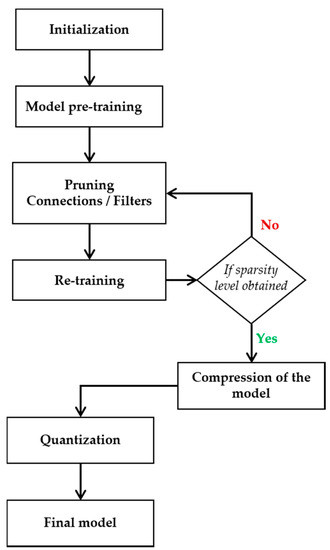
Figure 2. Flowchart of model pruning and quantization.

4.1. Initialization

As proposed in [44], we implement the removal of the weights using a mask tensor ($\mathit{M}$) initialized at 1 at the early stage of the training, and of the same size as the weight tensor ($\mathit{W}$).

4.2. Pretraining

The first training phase performs a normal Stochastic Gradient Descent (SGD). The L2-normalization allows to reduce the magnitude of the weights and also rank them in order of importance.

4.3. Pruning

The connections are pruned iteratively by defining a step sparsity level at each stage. A polynomial decay function is used to determine the step sparsity level. It is defined in Equation (4).

$$SSL=S+\left(S_r-S\right)\left(1- \frac{k-r}{r-n}\right)$$

(4)

where $S$ is the targeted sparsity level; $S_r$ the initial sparsity level, $r$ the initial iteration, $n$ the last iteration, and k the current iteration. The step sparsity level is used to determine the threshold value of important connections.

To determine the threshold, the weights of each layer are ranked according to their magnitude. The threshold value is the value at the position step sparsity level multiplied by the number of weights. Let us consider $m_{ij}$ an element of the mask tensors $\mathit{M}$, when the absolute value of the weight associated to $m_{ij}$ is below the threshold $T$, $m_{ij}$ takes the value 0 as defined by Equation (5). The dot product given in Equation (6) forces the pruned weights to be set to zero.

$$m_{ij}=\{\begin{array}{c}0 if \left|w_{ij}\right|<T\\ 1 otherwise\end{array}$$

(5)

$$\mathit{W}=\mathit{W}.\mathit{M}$$

(6)

Unlike the connections pruning, in filters pruning, the salience criteria is the value of the sum of the absolute values of the filter weights. All the values in the mask corresponding to the weight of each filter are set to 0 if the sum of the absolute values of its filter weights is less than the threshold as defined in Equation (7). Then the dot product given in Equation (6) forces the pruned weights to be set to zero.

$$\mathit{M}= 0 if {\displaystyle \sum }_{filters}\left|\mathit{W}\right|< T$$

(7)

4.4. Retraining

The retraining of the model allows to correct the damage caused by the removal of connections. After each backpropagation the weights of pruned connections are reset to zero by the dot product in Equation (6).

4.5. Compression of the Model

At this step we can either compress the size of the weights or extract the reduced architecture of the model. Since the weights are zeroed in an unstructured fashion, they cannot be removed from the layer weight tensor. Compressing the model file allows us to observe the variation in size. We use Gzip for file compression.

After retraining, connections with null masks can be directly removed from the model architecture.

Convolutional layers: each filter is removed if its mask consists of zero values. Channels corresponding to the pruned filters are deleted in the next layers entry.

Batch-normalization layers: In the normalization layers the channels corresponding to the pruned filters are also deleted.

Soft-Max layer: removal of filters at the last convolution layer also requires removal of the corresponding connections in the soft-Max layer.

4.6. Quantization

We adopt quantization only at post-training. We apply fixed-point weights quantization. The matrix of weights is compressed from 32- to 16-bit floating point values.

5. Datasets and Experimentation Setup

5.1. Datasets

We conducted a set of experiments using two datasets of plant, namely plant seedlings dataset (V2) and Flavia database. The plant seedlings database [12] is a public image database for benchmark of plant seedling classification. The dataset contains 5537 images of 5184 × 3456 pixels of crop plants and weeds all in the seedling stage. The database includes 12 species of Danish agricultural plants and weeds with 253–762 images per species. Images of the different plants were collected with a DSLR camera at different stages separated by 2–3 days. Here we randomly selected 80% of images for training and 20% of images for evaluation. The second dataset (Flavia dataset) consists of 1907 leaf images of 1600*1200 pixels of 32 different plant species with 50–77 images per species [13]. Each image contains a single trimmed and isolated leaf. The images were collected on the campus of the Nanjing University and the Sun Yat-Sen arboretum using scanners or digital cameras on a plain background. The provided database contains RGB color images with a white background. We also randomly selected 80% of images for training and 20% of images for evaluation.

5.2. Experimentation Setup

We performed both parameters pruning and quantization on the LeNet5, AlexNet, and VGG-16. For each model, we modified only the last layer with respect to the number of classes in the dataset. For training we used the Stochastic Gradient Descent with a learning rate of ${10}^{-2}$. For these three experiments, we used softmax output layer with categorical cross-entropy loss. We trained both simple models and compressed models over 100 epochs using the training-set plant seedlings dataset and 500 epochs for Flavia database because of its small number of images. The input images were all resized to (50 × 50) without any data augmentation process.

5.3. Pruning

In the experiments we used iterative pruning and $L_2$ normalization. The pruning was performed after each 100 iterations of 50 images per batch. Then less relevant connections were set to zero according to the magnitude and the step sparsity level. The first iteration of pruning removes 50% of parameters, then continues gradually to achieve the desired sparsity level. The first iteration of pruning was performed after 1/5 of the total number of epochs. In addition, 1/10 of total epochs was used to allow the model to recover from the accuracy drop.

5.3.1. Experimentation Setting 1

The first experiment consists of performing the pruning on each layer of the model in order to obtain a completely sparse model. Each layer has the same sparsity level with $L_2$ regularization. For the same model we observed the accuracies in four cases. We removed 80%, 85%, 90%, and 95% of parameters.

5.3.2. Experimentation Setting 2

Convolutional layers use less weight than fully connected layers due to parsimony and weight sharing. Therefore, if the model is not too deep, these layers do not represent much of the overall volume of the model weights. For this experiment, the pruning is mainly focused on the fully connected module of our models. We first undertook a study of the proportions of dense layers in the total number of model parameters.

5.3.3. Experimentation Setting 3

The third experiment consists of filter-level pruning. Here to simplify the architecture, we replaced the fully connected module with a Global Average Pooling layer and a softmax layer. The new model (Model + GAP) was pruned with the total weights sum. The filter magnitude was determined by the absolute value of the weights sum.

6. Evaluation

To evaluate the performances of model pruning and quantization as model compression for agricultural applications, we focused on the reduction of the memory footprint and the speed-up. The core algorithms for fine-grained pruning and filter-level pruning are provided in Appendix A and Appendix B respectively.

6.1. Pruning with Same Pruning Ratio per Layer

Table 2, Table 3 and Table 4 present the application of pruning followed by a postquantization on the plant seedlings dataset for models VGGNet16, AlexNet, LeNet5, respectively. The comparison was made in terms of size and accuracy at different pruning levels. Results show that by using pruning techniques during compression and postquantization we can reduce the size of the models by an average factor of 38. In other words, we can achieve a reduction of factor 3.5, 4.2, 5.3, and 7.5 by removing, respectively, 80%, 85%, 90%, and 95% of trainable weights without considerable variation. We can then apply the postquantization and obtain a reduction of factor 12, factor 16, factor 22, and factor 38 with the same precision. In all the following tables, bold numbers indicate the best accuracy.

Table 2. Comparison in terms of size before and after compression on VGGNet16 and the plant seedlings dataset.

VGGNet16	Original	80% Pruning	85% Pruning	90% Pruning	95% Pruning
Pruning
Size	152.61 Mb	43.47 Mb	36.12 Mb	28.45 Mb	20.17 Mb
Accuracy	88.67	88.40	89.48	86.88	88.85
Pruning + postquantization
Size	36.76 Mb	11.84 Mb	9.41 Mb	6.87 Mb	3.98 Mb
Accuracy	88.67	88.23	89.03	89.84	89.03

Table 3. Comparison in terms of size before and after compression on AlexNet and the plant seedlings dataset.

AlexNet	Original	80% Pruning	85% Pruning	90% Pruning	95% Pruning
Pruning
Size	131.25 Mb	37.27 Mb	30.95 Mb	24.40 Mb	17.40 Mb
Accuracy	86.70	87.24	87.87	86.88	87.96
Pruning + postquantization
Size	32.37 Mb	10.18 Mb	8.09 Mb	5.89 Mb	3.42 Mb
Accuracy	86.97	86.70	88.31	86.61	87.78

Table 4. Comparison in terms of size before and after compression on LeNet5 and the plant seedlings dataset.

LeNet5	Original	80% Pruning	85% Pruning	90% Pruning	85% Pruning
Pruning
Size	42.54 Mb	12.02 Mb	10.01 Mb	7.91 Mb	5.65 Mb
Accuracy	83.56	84.28	80.14	83.38	83.11
Pruning + postquantization
Size	9.91 Mb	3.17 Mb	2.49 Mb	1.86 Mb	1.10 Mb
Accuracy	83.55	84.36	82.65	83.55	84.09

We obtained similar results by applying the same process on the Flavia database. Since only the last layer is changed in the architecture of the models applied to these two datasets, the variation in terms of size is exceedingly small. Table 5 presents the different accuracy values obtained by applying the pruning on LeNet5, AlexNet, and VGG16 with a sparsity level of 80%, 85%, 90%, and 95% for all the architectures.

Table 5. Comparison in terms accuracy before and after compression on the Flavia database.

Models	Accuracy	80% Pruning	85% Pruning	90% Pruning	95% Pruning
Pruning
VGG16	91.36	87.70	90.58	90.88	91.49
AlexNet	96.07	96.86	97.9	97.9	95.81
LeNet5	95.03	94.76	92.41	94.76	95.03
Pruning + postquantization
VGG16	91.49	84.28	80.14	83.38	83.11
AlexNet	96.59	96.59	97.9	97.9	95.54
LeNet5	95.02	94.50	92.67	95.81	95.02

6.2. Only Fully Connected Layers Pruning

Figure 3 presents the distribution of the number of parameters for LeNet5 (top-panel), AlexNet (middle-panel), and VGGNet16 (botton-panel). Between the different convolutional layers, we have Pooling and Batch-Normalization layers that have insignificant weights, as well as the Drop-out layer between the fully connected layers. The convolutional layers have less weight than the fully connected layers. This is mainly due to the weight sharing and local connectivity of the neurons. Unlike AlexNet and LeNet5, VGGNet16 still has a considerable number of weights in the convolutional layers. Although the kernels are very small the convolutional layers have a large number of filters in VGGNet16. Figure 4 shows a comparison of fully connected layers to the rest of the neural network.

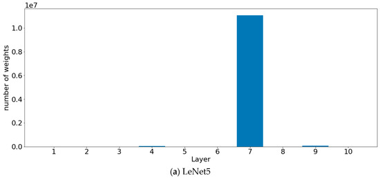
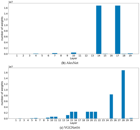
Figure 3. Weights histogram.

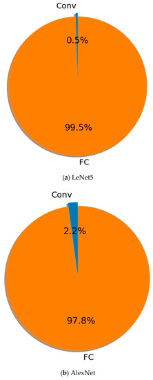
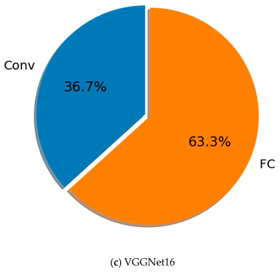
Figure 4. Weights sum for fully connected layers (orange) and convolutional layers (blue).

Between the different convolutional layers, we have Pooling and Batch-Normalization layers that have insignificant weights, as well as the Drop-out layer between the fully connected layers. The convolutional layers have less weight than the fully connected layers. This is mainly due to the weight sharing and local connectivity of the neurons. Unlike AlexNet and LeNet5, VGGNet16 still has a considerable number of weights in the convolutional layers. Although the kernels are very small the convolutional layers have a large number of filters in VGGNet16.

Dense layers have an exceptionally large number of parameters, which greatly influence the size of the model. Here, the convolutional layers are not pruned during training. Table 6, Table 7 and Table 8 present the results obtained after 99% pruning of the weights of the fully connected (FC) layers of models VGGNet16, AlexNet, LeNet5, respectively.

Table 6. Comparison in terms of size and accuracy before and after compression of the VGGNet FC-layer on the plant seedlings database.

VGG16	Original	99% FC Pruning
Pruning
Size	152.61 Mb	59.36 Mb
Accuracy	88.67	80.68
Pruning + postquantization
Size	36.76 Mb	13.83 Mb
Accuracy	88.67	80.05

Table 7. Comparison in terms of size and accuracy before and after compression of AlexNet FC-layer on the plant seedlings database.

AlexNet	Original	99% FC Pruning
Pruning
Size	131.25 Mb	6.21Mb
Accuracy	86.70	88.49
Pruning + postquantization
Size	32.37 Mb	1.54 Mb
Accuracy	86.97	88.85

Table 8. Comparison in terms of size and accuracy before and after compression of LeNt5 FC-layer on the plant seedlings database.

LeNet5	Original	99% FC Pruning
Pruning
Size	42.54 Mb	3.54 Mb
Accuracy	83.56	82.25
Pruning + postquantization
Size	9.91 Mb	0.86 Mb
Accuracy	83.55	86.70

On VVGNet16, by using only 1% of weights in the fully connected layers, the model size is reduced by factor 2.5 with a drop of 7.99 in terms of accuracy. By combining pruning and quantization, the model is reduced by factor 11 with the same accuracy drop of 7.99.

With AlexNet (see Table 7), using only 1% of weights in the fully connected layers, the model size is reduced by a factor of 21.1 with a gain in accuracy of 1.79. By combining pruning and quantization, the model is reduced by a factor of 85.2 with a gain in accuracy of 2.15.

Using LeNet5 (see Table 8), only 1% of weights in the fully connected layers is used. The model size is reduced by factor 12.01 with a drop of 1.3 in accuracy. However, by combining pruning and quantization, the model is reduced by factor 49.4 with a gain in accuracy of 3.14.

By observing the above results, sometime pruning only the fully connected layers can be good enough if the goal is only the footprint reduction. Pruning only the fully connected layers with high sparsity level results in high compression of the whole model.

6.3. Filter Pruning

Table 9, Table 10 and Table 11 present the results of filter-level pruning on VGGNet, AlexNet, and LeNet5 associated with Global average pooling, applied on the plant seedlings dataset.

Table 9. Comparison in terms of size and FLOPs of filter-level pruning on VGGNet+GAP with the plant seedlings dataset.

VGGNet+GAP	Original	75% Pruning	80% Pruning	85% Pruning	90% Pruning
Filter-level pruning
Size	56.34Mb	3.56 Mb	2.33 Mb	1.34Mb	0.64 Mb
FLOPs	29,485,986	1,820,340	1,179,450	658,006	296,298
Accuracy	88.68	90.39	88.59	87.24	89.58
Pruning + postquantization
Size	14.09 Mb	0.89 Mb	0.58 Mb	0.33 Mb	0.16 Mb
Accuracy	88.85	90.38	88.40	87.33	89.84

Table 10. Comparison in terms of size and Flops of filter-level pruning on AlexNet+GAP with the plant seedlings dataset.

AlexNet+GAP	Original	75% Pruning	80% Pruning	85% Pruning	90% Pruning
Filter-level pruning
Size	2.93 Mb	0.234Mb	0.17 Mb	0.11 Mb	0.08 Mb
FLOPs	1,509,781	96,525	64,365	37,017	17,391
Accuracy	88.50	86.52	85.80	77.72	72.33
Pruning + postquantization
Size	0.73 Mb	0.06 Mb	0.04 Mb	0.03 Mb	0.02 Mb
Accuracy	88.31	86.16	86.25	77.62	72.32

Table 11. Comparison in terms of size and Flops of filter-level pruning on LeNet5+GAP with th plant seedlings dataset.

LeNet5+GAP	Original	75% Pruning	80% Pruning	85% Pruning	90% Pruning
Filter-level pruning
Size	349.97 Kb	63.55 Kb	52.8 Kb	43.8 Kb	36.8 Kb
FLOPs	167,367	20,403	15,787	10,863	6997
Accuracy	83.47	71.07	67.65	70.08	57.95
Pruning + postquantization
Size	86.05 Kb	15.42 Kb	12.95 Kb	12.66 Kb	9.23 Kb
Accuracy	83.55	71.06	68.10	69.36	54.80

Results show that the filter-level pruning is suitable for the VGGNet model and can compress it by a factor of 352 and accelerate it by a factor of 99 with a sparsity level of 90% while gaining in accuracy. On the other hand, AlexNet and LeNet5 are relatively smaller. The filter-level pruning seems to be less adapted. AlexNet can maintain a small loss of accuracy with a sparsity level of 80%, but LeNet5 with a sparsity level of 75% loses considerably in terms of accuracy.

6.4. Input Layer Resizing

The size of the input image is also an important parameter in the architecture of the model. The optimal choice of the input image considerably reduces the size of the model. Table 12 presents the use of VGGNet16 on the plant seedlings dataset with different sizes of input layers.

Table 12. Size of VGGNet16 with different sizes of the input image from the plant seedlings dataset.

VGGNet16 Input Size	Size	Accuracy
224 × 224 × 3	512.91 Mb	93.19
100 × 100 × 3	248.91 Mb	94.24
50 × 50 × 3	152.91 Mb	93.97

The use of input images of size $50 \times 50 \times 3$ instead of $224 \times 224 \times 3$ as proposed by [6] on ImageNet, can allow us to have a model more than three times smaller with VGG16.

7. Conclusions and Future Work

In this paper, we raised the interest of DL model compression in the application to plant disease detection in agriculture. We discussed the DL inference on low-resources devices, then we summarized important techniques for size compression and consequently times speed-up which have been applied to allow DL on devices with limited resources. To evaluate the performance of model compression, we applied two pruning methods, combined with quantization to compress LeNet5, VGG16, and AlexNet on two databases used in agriculture. The results show on one hand that it is possible with fine-grained pruning to compress the size of these models by an average factor of 38 by pruning 95% of the model. Additionally, that in some cases only 1% of the weight of the fully connected layers can be used. However, deployment requires the use of specialized hardware. On the other hand, filter-level pruning can compress the size of huge models such as VGGNet by a factor of 352 and accelerate it by a factor of 99, without considerable accuracy loss. However, it is less efficient on smaller models.

Filter-level pruning has the advantage of directly reducing the architecture of the model which allows it to be deployed directly in farms on limited resources such as Arduino Yun (64 MB), Raspberry Pi (256 MB-1 GB), drones, and smartphones. In future work, we will experiment with fine-grained pruning in real farming environments using resources such as EIEs (Efficient Inference Engine) and FPGAs (Field Programmable Gate Arrays) to speed-up pruned model inferences.

References

- Kamilaris, A.; Prenafeta-Boldú, F.X. Deep learning in agriculture: A survey. Comput. Electron. Agric. 2018, 147, 70–90. [Google Scholar] [CrossRef]
- Zheng, Y.-Y.; Kong, J.-L.; Jin, X.-B.; Wang, X.-Y.; Su, T.-L.; Zuo, M. CropDeep: The crop vision dataset for deep-learning-based classification and detection in precision agriculture. Sensors 2019, 19, 1058. [Google Scholar] [CrossRef] [PubMed]
- Jin, X.-B.; Yu, X.-H.; Wang, X.-Y.; Bai, Y.-T.; Su, T.-L.; Kong, J.-L. Deep learning predictor for sustainable precision agriculture based on internet of things system. Sustainability 2020, 12, 1433. [Google Scholar] [CrossRef]
- Zhang, C.; Patras, P.; Haddadi, H. Deep learning in mobile and wireless networking: A survey. IEEE Commun. Surv. Tutor. 2019, 21, 2224–2287. [Google Scholar] [CrossRef]
- Zhang, L.; Jia, J.; Gui, G.; Hao, X.; Gao, W.; Wang, M. Deep learning based improved classification system for designing tomato harvesting robot. IEEE Access 2018, 6, 67940–67950. [Google Scholar] [CrossRef]
- Rahnemoonfar, M.; Sheppard, C. Deep count: Fruit counting based on deep simulated learning. Sensors 2017, 17, 905. [Google Scholar] [CrossRef]
- Ebongue, J.L.F.K. Rethinking Network connectivity in rural communities in Cameroon. arXiv 2015, arXiv:1505.04449. [Google Scholar]
- Fendji, J.; Thron, C.; Nlong, J.M. Mesh router nodes placement in rural wireless mesh networks. In Proceedings of the CARI, Saint Louis, Senegal, 16-23 October 2014; pp. 265–272. [Google Scholar]
- Shi, W.; Cao, J.; Zhang, Q.; Li, Y.; Xu, L. Edge computing: Vision and challenges. IEEE Internet Things J. 2016, 3, 637–646. [Google Scholar] [CrossRef]
- Atanbori, J.; French, A.P.; Pridmore, T.P. Towards infield, live plant phenotyping using a reduced-parameter CNN. Mach. Vis. Appl. 2020, 31, 2. [Google Scholar] [CrossRef]
- Atanbori, J.; Chen, F.; French, A.P.; Pridmore, T.P. Towards Low-Cost Image-Based Plant Phenotyping Using Reduced-Parameter CNN. In Proceedings of the 29th British Machine Vision Conference, Newcastle upon Tyne, UK, 4–6 September 2018; pp. 98–107. [Google Scholar]
- Giselsson, T.M.; Jørgensen, R.N.; Jensen, P.K.; Dyrmann, M.; Midtiby, H.S. A public image database for benchmark of plant seedling classification algorithms. arXiv 2017, arXiv:1711.05458. [Google Scholar]
- Wu, S.G.; Bao, F.S.; Xu, E.Y.; Wang, Y.-X.; Chang, Y.-F.; Xiang, Q.-L. A leaf recognition algorithm for plant classification using probabilistic neural network. In Proceedings of the 2007 IEEE International Symposium on Signal Processing and Information Technology, Giza, Egypt, 15–18 December 2007; pp. 11–16. [Google Scholar]
- LeCun, Y.; Bottou, L.; Bengio, Y.; Haffner, P. Gradient-based learning applied to document recognition. Proc. IEEE 1998, 86, 2278–2324. [Google Scholar] [CrossRef]
- Krizhevsky, A.; Sutskever, I.; Hinton, G.E. ImageNet classification with deep convolutional neural networks. In Proceedings of the Advances in Neural Information Processing Systems, Lake Tahoe, NV, USA, 3–8 December 2012. [Google Scholar]
- Simonyan, K.; Zisserman, A. Very deep convolutional networks for large-scale image recognition. arXiv 2014, arXiv:1409.1556. [Google Scholar]
- He, K.; Zhang, X.; Ren, S.; Sun, J. Deep residual learning for image recognition. In Proceedings of the IEEE Conference on Computer Vision and Pattern Recognition, Las Vegas, NV, USA, 26 June–1 July 2016; pp. 770–778. [Google Scholar]
- Szegedy, C.; Vanhoucke, V.; Ioffe, S.; Shlens, J.; Wojna, Z. Rethinking the inception architecture for computer vision. In Proceedings of the IEEE Conference on Computer Vision and Pattern Recognition, Las Vegas, NV, USA, 26 June–1 July 2016; pp. 2818–2826. [Google Scholar]
- Tzounis, A.; Katsoulas, N.; Bartzanas, T.; Kittas, C. Internet of things in agriculture, recent advances and future challenges. Biosyst. Eng. 2017, 164, 31–48. [Google Scholar] [CrossRef]
- Lane, N.D.; Bhattacharya, S.; Mathur, A.; Forlivesi, C.; Kawsar, F. DXTK: Enabling resource-efficient Deep learning on mobile and embedded devices with the DeepX toolkit. In Proceedings of the 8th EAI International Conference on Mobile Computing, Applications and Services, Cambridge, UK, 30 November–1 December 2016; pp. 98–107. [Google Scholar]
- Lee, S.H.; Chan, C.S.; Wilkin, P.; Remagnino, P. Deep-plant: Plant identification with convolutional neural networks. In Proceedings of the 2015 IEEE International Conference on Image Processing (ICIP), Quebec City, QC, Canada, 27–30 September 2015; pp. 452–456. [Google Scholar]
- Yalcin, H. Plant phenology recognition using deep learning: Deep-Pheno. In Proceedings of the 2017 6th International Conference on Agro-Geoinformatics, Fairfax, VA, USA, 7–10 August 2017; pp. 1–5. [Google Scholar]
- Mohanty, S.P.; Hughes, D.P.; Salathé, M. Using deep learning for image-based plant disease detection. Front. Plant. Sci. 2016, 7, 1419. [Google Scholar] [CrossRef] [PubMed]
- Dyrmann, M.; Karstoft, H.; Midtiby, H.S. Plant species classification using deep convolutional neural network. Biosyst. Eng. 2016, 151, 72–80. [Google Scholar] [CrossRef]
- Mortensen, A.K.; Dyrmann, M.; Karstoft, H.; Jørgensen, R.N.; Gislum, R. Semantic segmentation of mixed crops using deep convolutional neural network. In Proceedings of the International Conference of Agricultural Engineering (CIGR), Aarhus, Denmark, 26–29 June 2016. [Google Scholar]
- Christiansen, P.; Nielsen, L.N.; Steen, K.A.; Jørgensen, R.N.; Karstoft, H. DeepAnomaly: Combining background subtraction and deep learning for detecting obstacles and anomalies in an agricultural field. Sensors 2016, 16, 1904. [Google Scholar] [CrossRef]
- Bargoti, S.; Underwood, J. Deep fruit detection in orchards. In Proceedings of the 2017 IEEE International Conference on Robotics and Automation (ICRA), Singapore, 29 May–3 June 2017; pp. 3626–3633. [Google Scholar]
- Sa, I.; Ge, Z.; Dayoub, F.; Upcroft, B.; Perez, T.; McCool, C. Deepfruits: A fruit detection system using deep neural networks. Sensors 2016, 16, 1222. [Google Scholar] [CrossRef]
- Stein, M.; Bargoti, S.; Underwood, J. Image based mango fruit detection, localisation and yield estimation using multiple view geometry. Sensors 2016, 16, 1915. [Google Scholar] [CrossRef]
- Sladojevic, S.; Arsenovic, M.; Anderla, A.; Culibrk, D.; Stefanovic, D. Deep neural networks based recognition of plant diseases by leaf image classification. Comput. Intell. Neurosci. 2016, 6, 1–11. [Google Scholar] [CrossRef]
- Denil, M.; Shakibi, B.; Dinh, L.; Ranzato, M.; De Freitas, N. Predicting parameters in deep learning. In Proceedings of the Advances in Neural Information Processing Systems, Lake Tahoe, NV, USA, 5–10 December 2013; pp. 2148–2156. [Google Scholar]
- Ba, J.; Caruana, R. Do deep nets really need to be deep? In Proceedings of the Advances in Neural Information Processing Systems, Montreal, QC, Canada, 8–13 December 2014; pp. 2654–2662. [Google Scholar]
- Han, S.; Pool, J.; Tran, J.; Dally, W. Learning both weights and connections for efficient neural network. In Proceedings of the Advances in Neural Information Processing Systems, Montreal, QC, Canada, 7–12 December 2015; pp. 1135–1143. [Google Scholar]
- Lee, N.; Ajanthan, T.; Torr, P.H. Snip: Single-shot network pruning based on connection sensitivity. arXiv 2018, arXiv:1810.02340. [Google Scholar]
- Wen, W.; Wu, C.; Wang, Y.; Chen, Y.; Li, H. Learning structured sparsity in deep neural networks. In Proceedings of the Advances in Neural Information Processing Systems, Barcelona, Spain, 5–10 December 2016; pp. 2074–2082. [Google Scholar]
- LeCun, Y.; Denker, J.S.; Solla, S.A. Optimal brain damage. In Proceedings of the Advances in Neural Information Processing Systems, Denver, Colorado, USA, 26–29 November 1990; pp. 598–605. [Google Scholar]
- Hassibi, B.; Stork, D.G.; Wolff, G.J. Optimal brain surgeon and general network pruning. In Proceedings of the IEEE International Conference on Neural Networks, San Francisco, CA, USA, 28 March–1 April 1993; pp. 293–299. [Google Scholar]
- Gupta, M.; Aravindan, S.; Kalisz, A.; Chandrasekhar, V.; Jie, L. Learning to Prune Deep Neural Networks via Reinforcement Learning. arXiv 2020, arXiv:2007.04756. [Google Scholar]
- Banerjee, B. Pruning for Monte Carlo Distributed Reinforcement Learning in Decentralized POMDPs. In Proceedings of the AAAI, Bellevue, WA, USA, 14–18 July 2013. [Google Scholar]
- Mao, H.; Han, S.; Pool, J.; Li, W.; Liu, X.; Wang, Y.; Dally, W.J. Exploring the regularity of sparse structure in convolutional neural networks. arXiv 2017, arXiv:1705.08922. [Google Scholar]
- Ge, S. Efficient deep learning in network compression and acceleration. In Digital Systems; IntechOpen: London, UK, 2018. [Google Scholar]
- Lebedev, V.; Lempitsky, V. Fast convnets using group-wise brain damage. In Proceedings of the Proceedings of the IEEE Conference on Computer Vision and Pattern Recognition, BLas Vegas, NV, USA, 26 June–1 July 2016; pp. 2554–2564. [Google Scholar]
- Luo, J.-H.; Wu, J.; Lin, W. Thinet: A filter level pruning method for deep neural network compression. In Proceedings of the IEEE International Conference on Computer Vision, Venice, Italy, 22–29 October 2017; pp. 5058–5066. [Google Scholar]
- Zhu, M.; Gupta, S. To prune, or not to prune: Exploring the efficacy of pruning for model compression. arXiv 2017, arXiv:1710.01878. [Google Scholar]
- Howard, A.G.; Zhu, M.; Chen, B.; Kalenichenko, D.; Wang, W.; Weyand, T.; Andreetto, M.; Adam, H. Mobilenets: Efficient convolutional neural networks for mobile vision applications. arXiv 2017, arXiv:1704.04861. [Google Scholar]
- Chollet, F. Xception: Deep learning with depthwise separable convolutions. In Proceedings of the Proceedings of the IEEE Conference on Computer Vision and Pattern Recognition, Honolulu, HI, USA, 21–26 July 2017; pp. 1251–1258. [Google Scholar]
© 2020 by the authors. Licensee MDPI, Basel, Switzerland. This article is an open access article distributed under the terms and conditions of the Creative Commons Attribution (CC BY) license (http://creativecommons.org/licenses/by/4.0/).