A Fast Laser Adjustment-Based Laser Triangulation Displacement Sensor for Dynamic Measurement of a Dispensing Robot

Abstract

Height measurement and location by a laser sensor is a key technology to ensure accurate and stable operation of a dispensing robot. In addition, alternation of dynamic and static working modes of a robot, as well as variation of surface and height of a workpiece put forward strict requirements for both repeatability and respond speed of the location system. On the basis of the principle of laser triangulation, a displacement sensor applied to a dispensing robot was developed, and a fast laser adjustment algorithm was proposed according to the characteristics of static and dynamic actual laser imaging waveforms on different objects. First, the relationship between the centroid position of static waveform and peak intensity for different measured objects was fitted by least square method, and the intersection point of each curve was solved to confirm the ideal peak intensity, and therefore reduce the interference of different measured objects. Secondly, according to the dynamic centroid difference threshold of two adjacent imaging waveforms, the static and dynamic working modes of the sensor were distinguished, and the peak intensity was adjusted to different intervals by linear iteration. Finally, a Z direction reciprocating test, color adaptability test, and step response test were carried out on the dispensing robot platform; the experiments showed that the repeatability accuracy of the sensor was 2.7 um and the dynamic step response delay was 0.5 ms.

1. Introduction

With the development of modern science and technology, miniaturization of intelligent equipment has become a trend, which puts forward more stringent requirements for the processing technology of the equipment. In order to ensure the reliability of equipment processing, protective measures need to be taken. Precision dispensing technology effectively solves this problem and is widely used in many fields such as bottom filling, precision coating, chip encapsulation, component fixation, and so on [1,2,3].

Traditional precision dispensing depends on manual work under a microscope [4], which has the disadvantages of low production efficiency, high work intensity, and inevitable human error. With the continuous development of automation and robot technology, a series of dispensing robots have been developed to improve dispensing efficiency. All the dispensing robots developed by the Nordson Corporation (USA), the Datron Corporation (Germany), and the Soonchunhyang University (Korea) [5,6] have realized automatic high-speed precision dispensing, but the price has been expensive and they have been costly to maintain. Therefore, development of a high-precision and low-cost dispensing robot has potential application prospects. The location technology of the dispensing robot is the key to ensure measurement accuracy. Generally, height information of the actuator relative to the workpiece is accurately fed back to a robot through the photoelectric detection system, in order to carry out the operation [7,8].

A laser triangulation displacement sensor (LTDS) is a kind of ranging sensor which combines high directivity and brightness of laser with the principle of triangular measurement. It has the advantages of wide application, large measuring range, high precision, and fast response [9,10,11,12], and can be applied for precisely measuring the height information of a dispensing robot. Considering the working environment of a dispensing robot, the technical difficulties to be overcome when using LTDS to detect dispensing height information are as follows:

• The problem of the adaptability of different objects, i.e., the different textures and colors of an object on the dispensing substrate affect the measurement, and the sensor must have good adaptability to different objects;
• The problem of dynamic response speed, i.e., dispensing is a high-speed dynamic process, because the height of the workpiece on the dispensing substrate is not uniform, the sensor should have fast dynamic response speed during the measurement process.

Concerning the adaptability of different measured objects, for several years, researchers have studied the accuracy optimization methods of LTDS and have obtained a number of achievements. Klemen [13] introduced a dynamic symmetric projection and hyperbolic fitting compensation algorithm to solve robust alignment problems for different material objects, but the installation and measurement steps of this method were relatively complex. In contrast, it was relatively convenient to control the intensity of the laser imaging spot using an algorithm. Jung [14] improved the adaptability of the sensor to different colors by controlling the beam intensity of the laser diode so that the power received on the photoelectric device was constant when the object color changed. Similarly, Keyence [15] proposed the ABLE algorithm to adapt to the problem of light intensity inconsistency caused by different object colors. Song [16] established a mathematical model for the relationship between the imaging point position and the surface characteristic parameters of the measured object and modified the imaging point position according to the surface parameters to adapt to different measured objects. In addition, Li Sansi [17] analyzed the measurement error caused by different surface colors based on the Phong reflector model and established a color error function library to compensate for the error caused by the color change of the measured object. Although the above researches effectively improved the measurement accuracy of the LTDS for different objects, they did not involve the study of the dynamic response performance of the LTDS.

For the dynamic response speed problem, Zhang [18] developed a new type of LTDS which could measure the surface of a train with a speed of 64 km/h, but the accuracy was low. Scichi [19] proposed a dual-view triangulation structure to reduce the measurement error caused by the change of laser speckle when the measured object moved laterally. However, the structure was too large to be integrated. Thus, the LK-G series LTDS developed by Keyence [20,21] could achieve high-speed and high-precision measurement synchronously (50 KHz sampling frequency and accuracy of 0.05% F.S) through a highly integrated design. However, the LK-G series sensor took 4096 times, on average, to improve the measurement repeatability, and it relied on the sampling speed of customized imaging devices, with the disadvantage of complex steps that resulted in higher production costs.

In addition, imaging characteristics influence the accuracy of an optical measurement system. With the development of computer pattern recognition, researchers have carried out recognition and feature extraction for various optical images. Jeong [22] realized the detection of a dynamic laser spot by auto-associative multilayer perceptron (AAMLP) but did not extract the detailed information of the spot. Huffman [23] adopted a supervised classification algorithm based on a t-test filter for spectral feature classification in a complex data environment. Wang [24] proposed a method combining deep learning with a physical model to recover the information of the measured object from a single diffraction intensity diagram, but the imaging time of this method was too long. Manzo [25] developed an object recognition framework based on a fast convolution neural network, which could further extract more detailed features of the image and improved the speed of the model. Although the above studies had forward-looking significance, they had high requirements for the performance of the hardware system, which was not conducive to integrated development and promotion of LTDS. Therefore, we need a simpler laser imaging recognition method that requires less hardware. Moreover, in the particular application of a dispensing robot, it is necessary to quickly distinguish the dynamic and static imaging and to adjust the imaging to ensure measurement accuracy.

In this paper, an LTDS was proposed for a dispensing robot. By using the adjustment algorithm of laser imaging waveform, a method of “replacing hardware with software” was adopted to save hardware cost, and high-precision measurements in a dynamic scene were realized to meet the application requirements of a dispensing robot. First, the principle of dispensing robot system and the laser spot location method of the LTDS were introduced. Secondly, from the static and dynamic point of view, we studied the characteristics of an actual laser imaging waveform, in which the measured objects were a white diffuse reflector and a black frosted reflector, respectively. The optimal peak intensity of the imaging waveform was determined by least square fitting. Then, considering the actual working scene of a dispensing robot, a fast waveform adjustment algorithm was proposed. According to the dynamic centroid position shift of the imaging waveform, the static and dynamic working modes of the sensor were distinguished, and the peak intensity of the waveform was adjusted to different intervals by linear iteration. Finally, based on the dispensing robot experimental platform, we verified the repeatability accuracy and the step dynamic response characteristics of the sensor.

2. Dispensing Robot System and Laser Spot Location Principle

2.1. Principe of the Dispensing Robot System

The location and height measurement system of the dispensing robot is shown in Figure 1. The LTDS was fixed on the end of the manipulator to measure the workpiece in real time. It was designed based on direct-injection laser triangulation imaging [26]. The laser light emitted by a laser diode (LD) was focused by a collimated lens and projected vertically onto the object to form reflected light. The reflected light propagated in space by way of diffuse reflection, and then the reflected light was focused by the receiver lens in the direction of the observation angle ε and formed a laser imaging spot on the photosensitive imaging device (CMOS). The position of the imaging spot on the CMOS was obtained by the spot location algorithm. When the object moves s, the position of the imaging spot moves Δx on the CMOS accordingly, and the displacement s can be calculated according to Equation (1), where l and f_po are the object distance and image distance of the receiver lens group, and β is the imaging angle:

$$s=\frac{\Delta x\cdot l\sin \beta }{f_{po}\cdot \sin \epsilon -\Delta x\cdot l\sin \left(\alpha +\beta \right)}$$

(1)

During the high-speed movement when the dispensing robot was working, the surface and height of the workpiece could suddenly change, which inevitably led to distortion of the laser imaging spot and reduced the measurement accuracy. The different surfaces and heights of the workpiece led to a change in the shape and position shift of the imaging waveform, respectively. According to the characteristics of an actual imaging waveform, considering the static and dynamic working mode of the robot, we proposed a fast laser intensity iterative adjustment method to obtain an ideal waveform for laser spot location, in order to satisfy measurement accuracy and response speed in both.

2.2. Laser Imaging Spot Location

The laser spot location algorithm is the most important key technology to improve measurement accuracy. The gray centroid method [27,28] and function fitting method [29,30,31,32] are the mainstream methods. Under ideal conditions, the laser spot energy presents a Gaussian distribution. The function fitting method fits the Gaussian distribution of the spot energy by a simplified mathematical function, which can effectively and quickly obtain the position of the imaging point on the CMOS. In practice, however, due to optical distortion and the structure of the optical path, the imaging waveform was tilted and stretched, which led to a skewed distribution. Therefore, the function method causes some calculation deviation. In contrast, the gray centroid method can calculate the centroid of distorted waveforms to achieve the spot subpixel location.

To reduce the influence of random noise and increase the weight value near the peak, in this paper, the square weighted gray centroid method is adopted to calculate position x of the laser spot on the CMOS, as shown in Equation (2), where x_i is the position on the CMOS and y_i is the waveform intensity. In addition, we convert the position x from the pixel coordinates to the world coordinates by the calibration method of linear piecewise interpolation, and finally obtain the measured value.

$$x=\frac{{\sum }_i^N{x}_i\cdot y_i^2}{{\sum }_i^N{y}_i^2}$$

(2)

3. Characteristics of the Actual Laser Imaging Waveform

The quality of imaging waveform affects the result of the centroid calculation, thus the sensor developed, in this paper, adjusted the peak intensity of the imaging waveform by controlling the CMOS exposure time. In order to improve the efficiency of the adjustment algorithm and the adaptability to different objects, it was necessary to further analyze the characteristics of the imaging waveform.

3.1. Experiment Platform for Analyzing Imaging Waveform Characteristics

Although many practical factors, such as air flow, humidity, and temperature, have been considered in recent research on laser triangulation imaging [33,34], most of these researches have focused on simulation analysis and lacked complete analysis of the actual imaging waveform. In addition, there was a lack of research on the dynamic imaging waveform, so we comprehensively analyzed the actual laser imaging waveform from the static and dynamic perspectives.

An experimental platform for analysis of laser imaging waveform was established, as shown in Figure 2a. The LTDS developed, in this paper, was placed at a certain distance from the mobile platform. It was highly integrated with a field programmable gate array (FPGA) and STM32 microprocessor for signal processing. The key components in the sensor included a laser diode (Rohm Corporation, wavelength 650 nm, power 2 mw), a linear CMOS (Hamamatsu Corporation), and an optical lens, which were purchased without special customization, therefore, improving productivity and reducing costs. The measured object was fixed on the mobile platform (resolution 1 um and precision 2 um). When its movement was controlled by the motion controller, the imaging waveforms on the CMOS were collected synchronously by the host computer. The black frosted and white diffuse reflectors were selected as the measured objects to carry out the actual waveform analysis experiment, as shown in Figure 2b.

3.2. Characteristics of Static Laser Imaging Waveforms

By controlling the exposure time of the CMOS to obtain a gray-scale image, the characteristics of static imaging waveforms of two different measured object were studied. First, 10 groups of waveforms were obtained for two measured objects, and the change rule of waveform shape under different exposure times was analyzed. Then, the centroids of the waveforms were calculated, and the relationships among the centroid positions of the imaging waveform and the peak intensity were studied.

The imaging waveforms corresponding to different exposure times are shown in Figure 3. Although the imaging waveforms of the two different objects had obvious morphological differences (Figure 3a,b), the waveforms had a consistent trend when the peak intensity was in a certain range (350–800). The relationship between the exposure time and the peak intensity was further analyzed, as shown in Figure 3c. For different objects, the relationship between the peak intensity and the CMOS exposure time was different; the CMOS exposure time required to reach the target peak intensity could not be simply calculated from a function. Establishing multiple functions to calculate the CMOS exposure time for different measured objects was costly in terms of both software and hardware. Therefore, we intended to develop an iterative algorithm to automatically adjust the CMOS exposure time for different objects.

To confirm the ideal peak intensity, we considered the relationship between the peak intensity and the centroid position. As shown in Figure 4a, there was a certain difference in the centroid positions calculated from the waveforms with different peaks. To reduce this difference and to eliminate the interference caused by different colors, we fit the “centroid position-peak intensity” curve equation of black and white objects, respectively, as shown in Equation (3):

$$X\left(p\right)=a_k{p}^k+a_{k-1}{p}^{k-1}+a_{k-2}{p}^{k-2}+\cdots \cdots +a_{1}p+a_0$$

(3)

where a_k (k = 0, 1, 2, …) is the coefficient term, p is the peak intensity, and X (p) is the centroid position when the peak intensity was p.

The least square method is used to confirm the coefficient term, and the sum of squares of error I(a₀, a₁, …, a_k) is constructed, where C_i is the actual centroid position:

$$I\left(a_0,a_1,\cdots ,a_k\right)={{\displaystyle \sum _{i=1}^n\left[C_i-x\left(p_i\right)\right]}}^2={\displaystyle \sum _{i=1}^n\left(y_i-a_0-a_1{p}_1-\cdots -a_k{p}_i^k\right)}$$

(4)

Solving the corresponding coefficient a₀*, a₁*, …, a_k* such that:

$$I\left(a_0{}^{*},a_1{}^{*},\dots ,a_k{}^{*}\right)=\underset{a_0{}^{*},a_1{}^{*},\dots ,a_k{}^{*}}{\min }I\left(a_0,a_1,\dots ,a_k\right)$$

(5)

According to the least square approximation method described above, the centroid position-peak intensity equation can be written as:

$$\begin{array}{ll}X\left(p\right)& =\left[\begin{array}{c}{X}_w\\ X_b\end{array}\right]=\left[\begin{array}{c}1.216e-19\\ 5.878e-19\end{array}\right]p^7+\left[\begin{array}{c}-3.39e-16\\ -1.856e-15\end{array}\right]p^6+\left[\begin{array}{c}3.916e-13\\ 2.406e-12\end{array}\right]p^5\\ & +\left[\begin{array}{c}-2.574e-10\\ -1.649e-9\end{array}\right]p^4+\left[\begin{array}{c}1.178e-7\\ 6.383e-7\end{array}\right]p^3+\left[\begin{array}{c}-4.255e-5\\ -0.0001399\end{array}\right]p^2+\left[\begin{array}{c}0.01124\\ 0.01872\end{array}\right]p+\left[\begin{array}{c}568\\ 567.3\end{array}\right]\end{array}$$

(6)

where X_w and X_b are the centroid positions when the measured object is white diffuse reflector and black frosted reflector, and the intersection point of the equation curves is the ideal peak intensity (520 in this paper), as shown in Figure 4b.

3.3. Characteristics of Dynamic Laser Imaging Waveform

In order to study the change law of imaging waveform when the measured object moved, the mobile platform was driven by the host computer to enable the object to move 0.1 mm horizontally at a speed of 20 mm/s, which was a tiny displacement to avoid the interference caused by the texture change of the object surface, and five groups real-time imaging waveforms were collected (similar to static experiments, two different objects were selected). On the basis of the result of the static waveform experiment, we controlled the peak intensity of the imaging waveform to be as close as possible to the ideal value (520) by giving a constant CMOS exposure time.

The dynamic waveform change is shown in Figure 5. Although we tried to obtain a stable waveform by giving a constant exposure time, the imaging waveform was still distorted in the dynamic measurement process. Moreover, when the measured object was a black frosted reflector, the distortion of the imaging waveform changed more obviously than that of a white diffuse reflector, and the peak intensity oscillated violently. We considered that it was inevitable that the laser energy distribution on the CMOS was not uniform because of the superposition of light and the motion vector in the process of laser transmission. Therefore, it was necessary to develop a dynamic waveform adjustment strategy for dynamic waveform distortion.

Before developing the dynamic waveform adjustment algorithm, we quantitatively compared the static and dynamic waveforms, as shown in

Table 1. Change of centroid position and peak intensity of static and dynamic imaging waveforms.

	Centroid Shift (Pixels)		Intensity Difference (a.u.)
	Static	Dynamic	Static	Dynamic
White diffuse reflector	0.0259	0.5312	4	9
Black frosted reflector	0.0352	0.8641	4	28

. The peak intensity fluctuation of dynamic waveforms was two to seven times that of static waveforms, and the maximum centroid position shift was 24 times that of static waveforms. The peak intensity and centroid position drift of dynamic waveform were taken as the important indexes of dynamic waveform adjustment.

In summary, based on the analysis of actual imaging waveforms of laser on the CMOS, the characteristics of static and dynamic imaging waveforms were significantly different. Therefore, we needed to fully consider the difference between the two measurement scenarios to develop the control algorithm.

4. Fast Automatic Adjustment Algorithm of Imaging Waveform

On the basis of the characteristics of the static and dynamic actual imaging waveforms, and according to the centroid position shift of two adjacent frames of imaging waveforms, an automatic fast waveform adjustment algorithm was proposed. This method could satisfy the dynamic response of the dispensing robot during its high-speed motion, and could also ensure its static measurement accuracy. The algorithm flow is shown in Figure 6.

The proposed algorithm mainly included three main parts, i.e., waveform preprocessing, measurement mode judgment, and peak intensity adjustment which are described as follows: (1) The waveform preprocessing filtered out the noise interference and obtained the effective waveform information. (2) The measurement mode judgment determined whether the measurement mode was static or dynamic by setting the centroid difference threshold of two waveforms, and different peak intensity adjustment intervals were selected for these two measurement modes. (3) During the peak intensity adjustment part, a linear approximation prediction method was presented to quickly adjust the imaging waveform.

4.1. Imaging Waveform Preprocessing

Before entering the algorithm loop, we gave the initial CMOS exposure time T₀ to obtain the first frame image, and based on it, each subsequent waveform image was preprocessed as follows:

Step 1

Read the raw data of CMOS imaging waveform, identify the peak (P_i), and record its position x_p.

Step 2

To filter out the edge noise, select 15% of the peak intensity as the threshold, and the waveform whose energy is higher than the threshold is intercepted as the main peak.

Step 3

Apply a median smoothing filter to the main peak obtained by Step 2, taking into account both the filtering effect and speed.

4.2. Automatic Judgment of Measurement Mode

The actual working state of the dispensing robot alternated between dynamic and static. First, the dispensing robot moved to the target position at a high speed in the dynamic state, and then measured and dispensed in the static state.

Therefore, we set the dynamic centroid difference threshold between two adjacent frames of imaging waveform to distinguish the dynamic and static states and adopted different algorithm strategies. When it was the static working mode, the peak intensity was strictly controlled in an interval close to the ideal value (520), and therefore reduced the interference caused by different measured objects. Then, 64 times of smooth filter was applied to improve the measuring stability. In the dynamic mode, considering that the sharp fluctuation of the peak intensity of the dynamic waveform decreased the dynamic response speed of the sensor, we enlarged the peak intensity control interval. Different from the static mode, we did not filter the measured value in dynamic mode.

In the above algorithm, the dynamic centroid difference threshold and the peak intensity control interval of different working modes were identified as two important parameters.

4.2.1. Dynamic Centroid Difference Threshold

Table 1 shows the comparison of centroid shift of imaging waveforms between two adjacent frames, the centroid position shift caused by object motion is obvious, and the state of the measured object can be judged by the centroid difference. When the object moved, the centroid of the imaging waveform shifted at least 0.5312 pixel, therefore, we set the dynamic centroid difference threshold as 0.5 pixel. When the dynamic centroid difference was higher than 0.5 pixel, the sensor entered the dynamic mode. Otherwise, the sensor entered the static mode.

4.2.2. Peak Intensity Adjustment Interval

It was difficult to adjust the peak intensity to the ideal value at a time. Therefore, according to the static and dynamic working modes, different adjustment convergence intervals were determined to improve the peak intensity adjustment efficiency.

On the basis of the result of Equation (6), the “centroid position-peak intensity” fitting curve of different objects are subtracted to obtain the static centroid difference Xc(p) caused by the change of the peak intensity of different measured objects, as shown in Figure 7a, which was different from the dynamic centroid difference of two adjacent waveforms. We define the absolute deviation evaluation function ф(p), as shown in Equation (7), where φ is the deviation threshold. The peak intensity adjustment intervals under different working modes are determined according to φ:

$$\Phi \left(p\right)=\left|X_c\left(p\right)\right|=\left|X_b\left(p\right)-X_w\left(p\right)\right|\le \phi$$

(7)

When φ = 0.125 pixel, the corresponding dynamic peak intensity interval is [400,800], as shown in Figure 7b. When φ = 0.025 pixel, the corresponding static peak intensity interval is [500,550], as shown in Figure 7c. The pixel coordinates are converted to the world coordinates, the theoretical errors of dynamic and static measurement caused by φ are 2.7 um and 0.5 um respectively. Therefore, the selection of the above peak intervals satisfied the needs of high-precision measurement.

4.3. Peak Intensity Linear Iterative Adjustment

In order to further improve the convergence speed of peak intensity adjustment iteration, we proposed a linear iterative method, which simplified the exposure time and the peak intensity as a linear relationship, as shown in Figure 8. The relationship between the current waveform peak intensity and the ideal peak intensity was established, and the ideal peak intensity was approximated iteratively in the next frame.

First, we judge whether the waveform peak intensity Pi of the current frame is in the ideal interval. If it is in the ideal interval, no adjustment is needed, otherwise, the peak intensity adjustment is required. According to the coordinate point (T_i, P_i) consisting of the CMOS exposure time, T_i, and the peak intensity, P_i, a linear relationship is established, and the exposure time, T_i+1, required for the next frame is calculated from Equation (8) for waveform adjustment. This cycle is iterated until the peak intensity is adjusted to the ideal interval.

$$T_{i+1}=\frac{P_{i+1}}{P_i}{T}_i$$

(8)

In order to approach the ideal peak intensity, P_i+1, Equation (8) is replaced by the ideal peak intensity, P_c, as shown in Equation (9):

$$T_{i+1}=\frac{P_c}{P_i}{T}_i$$

(9)

where P_c is a constant, determined to be 520 by the analysis of the actual imaging waveform. On the basis of the above peak intensity linear iterative approximation method, the peak could be quickly adjusted to an ideal interval, and therefore improve the response performance of the sensor.

5. Dispensing Robot Experiment

5.1. Experimental Platform and Method

We verified the performance of the sensor developed in this paper on the dispensing robot platform by experiments. The DS-200C dispensing robot developed by the Mingseal Robot company (in China) was taken as the experimental platform, as shown in Figure 9a. The robot could move in three dimensions, i.e., X, Y, and Z. The maximum moving speeds in the X-Y direction and Z direction were 800 and 400 mm/s, respectively, and its repeat positioning accuracy was 10 um.

The sensor was fixed to the mechanical arm in the Z direction of the robot and different measured objects were placed on the X-Y platform (Figure 9b) for experiments, including the Z direction reciprocating test, color mutation adaptability test, and step response test. It should be noted that the robot stayed at each measured position for 30 ms to avoid interference caused by shaking of the manipulator. Considering the processing errors of the measured objects and the working table of the dispensing robot, the measurement performance of the sensor was evaluated for repeatability accuracy.

5.2. Z Direction Reciprocating Test Results and Analysis

To test the stability of the sensor in the Z direction of the dispensing robot, we fixed the sensor on the robot arm and moved back and forth at a speed of 400 mm/s along the Z direction, reaching five preset positions and staying for 30 ms, where the distance between each two-adjacent positions was 10 mm, as shown in Figure 10.

The displacement change curve of the sensor was recorded, as shown in Figure 11. When the sensor moved in the Z direction, its displacement curve was smooth and there was no obvious noise point, therefore, the sensor had good stability. Among them, the repeatability accuracy of five pause positions are shown in

Table 2. Repeatability accuracy of pause positions in the Z direction reciprocating test.

Position	Max Displacement (mm)	Min Displacement (mm)	Repeatability Accuracy (um)
1	61.0265	61.0251	1.4
2	52.2737	52.2719	1.8
3	42.0042	42.0034	0.8
4	52.2767	52.2746	2.1
5	61.0265	61.0249	1.6
Average	/	/	2.0

, with an average repeatability accuracy of 2 um.

5.3. Color Adaptability Test Results and Analysis

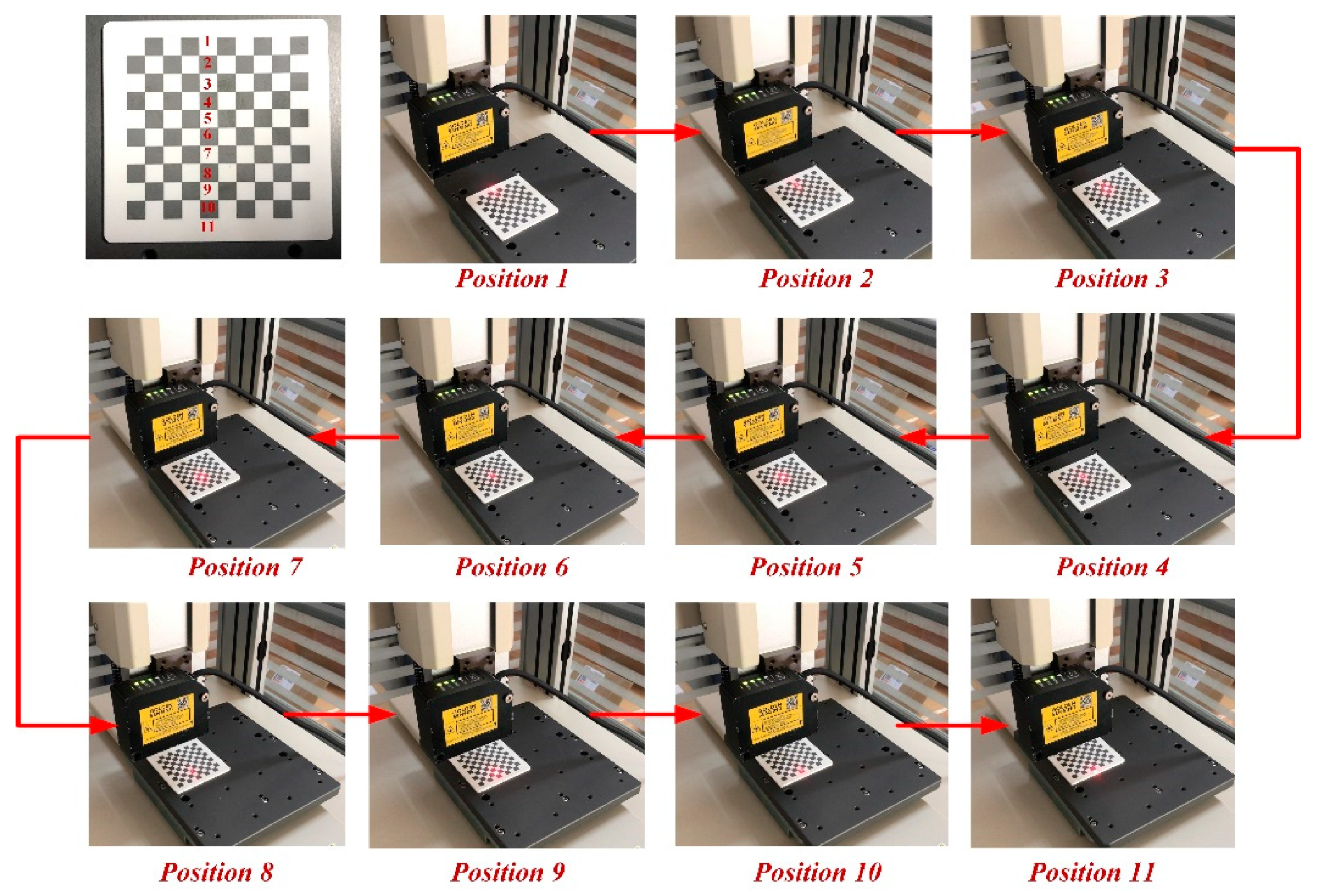
We placed a ceramic checkered calibration board (its total size was 50 × 50 mm, each square size was 5 × 5 mm, and surface flatness was 5 um) on the working platform of the dispensing robot. The black and white squares were used to simulate the scene of color mutation, and the adaptability of the sensor to the color of the measured object was tested.

As shown in Figure 12, we selected 11 alternate measured positions on the checkerboard for static and dynamic tests. First, the dispensing robot moved slowly to the measured positions. When the system was stable, the repeatability accuracy of each position was recorded, sequentially, in the static state. Then, the dynamic test was carried out, the dispensing robot moved at a speed of 800 mm/s, and it stopped for 30 ms at each measured position. The repeatability accuracy of each position during the short-time stay were also recorded, as shown in

Table 3. Repeatability accuracy test results when measured object color changed.

NO.	1	2	3	4	5	6	7	8	9	10	11	Average
Static (um)	0.9	0.5	1.5	0.3	1.6	0.3	1.4	5.4	0.8	1	1.9	1.42
Dynamic (um)	1.6	1	1	1.5	1.5	2.6	1.2	1.2	2.7	2.6	0.5	1.58

.

According to the results of Table 3, the dynamic measurement repeatability (1.58 um) of the sensor was very close to the static repeatability (1.42 um). This indicated that the sensor could quickly adjust to a stable working state within 30 ms under dynamic test conditions and verified that the sensor had good adaptability to the color dynamic change of the measured object.

5.4. Step Response Test Results and Analysis

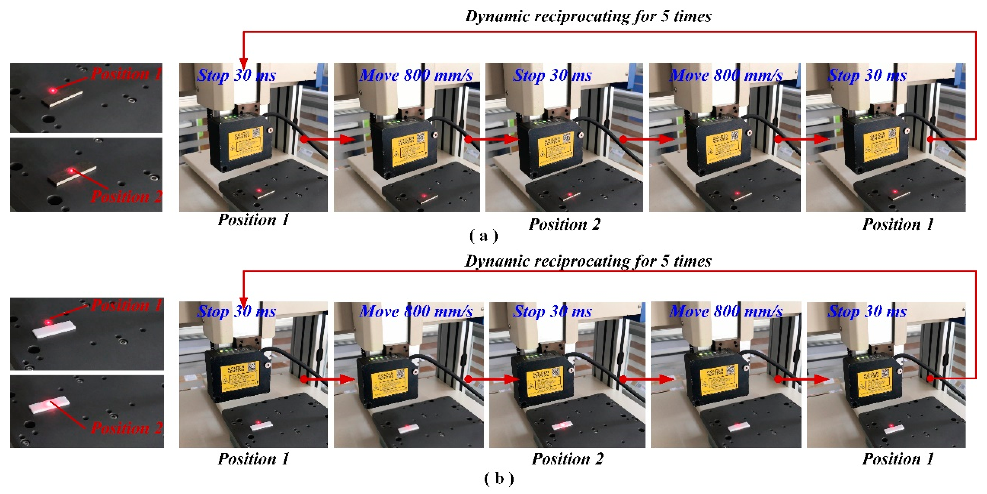
Two different steps were constructed for the step response test as follows: (1) A metal gauge block (2 mm in height, 10 mm in width, and 75 mm in length) was placed on the working table of the dispensing robot to construct a step without color change. (2) Similarly, a step with color change was constructed by a white ceramic gauge block (the same size as the metal gauge block). As shown in Figure 13, based on the steps constructed, the reciprocating dynamic experiments were conducted five times. The X-Y worktable of the robot moved at a speed of 800 mm/s, and stayed for 30 ms at the starting position (Position 1) and the measured position (Position 2) on the gauge block. During this process, the sensor recorded the data at a sampling frequency of 2 KHz.

First, we investigated the step response characteristics of the sensor in the dynamic test. As shown in Figure 14, the dynamic displacement curve of the sensor could completely express the changes of the two different steps’ height information, during the five reciprocating tests. However, there were obvious noise points at the edge of the step, which resulted in a delay of 0.5 ms for the measurement, therefore, the dynamic step response delay of the sensor we developed was 0.5 ms. We considered that there were two main reasons for the delay, one was the random tremble of the dispensing robot, the other was the instantaneous distortion of the laser spot when it moved from the worktable to the gauge block.

Furthermore, we investigated the repeatability accuracy of the sensor when it reached the measured position at a quick speed and passed through the step, as shown in

Table 4. Repeatability of measured position on the gauge block in the step dynamic reciprocating test.

No.	Metal Gauge Step			Ceramic Gauge Step
	Max (um)	Min (um)	R (um)	Max (um)	Min (um)	R (um)
1	48.8753	48.8706	4.7	48.9579	48.9569	1
2	48.8727	48.8707	2	48.9579	48.9565	1.4
3	48.8721	48.8706	1.5	48.9575	48.9559	1.6
4	48.8726	48.8703	2.3	48.9577	48.9558	1.9
5	48.8735	48.8704	3.1	48.9586	48.9571	1.5
Average	48.8732	48.8705	2.7	48.9579	48.9564	1.48

. The repeatability accuracies of the sensor for the metal gauge block and the ceramic gauge block were 2.7 um and 1.48 um, respectively, within 30 ms after the mechanical arm stopped, which met the needs of high-precision measurement.

To sum up, we verified the measurement repeatability and dynamic respond speed of the LTDS we proposed in various working scenarios of the dispensing robot through Z direction motion, color dynamic mutation. and step response experiments. The dynamic respond delay was 0.5 ms and the maximum repeatability error among the test scenarios was 2.7 um.

5.5. Comparison and Discussion

We added three different laser adjustment strategies for comparison, as shown in Figure 15. The laser adjustment method that only considered dynamic mode, the laser adjustment method that only considered static working mode, and the Proportional Integral Derivative (PID) control were selected, and these algorithms were implemented on a FPGA by program.

For the above different methods, we took the z direction stability, color adaptability, and step response tests, successively, under the same conditions (the measured object moved at the same speed). The measurement repeatability and dynamic response speed of each method were calculated. In addition, we defined the concept of positional noise density, σ, to comprehensively evaluate the accuracy and response speed of measurement, as shown in Equation (10).

$$\sigma =\sqrt{\frac{{\displaystyle \sum _{i=1}^n{\left(u_i-u\right)}^2}}{w}}$$

(10)

where u is the average measured displacement, u_i is the ith measured displacement, n is the total measured data, and w is the dynamic response speed. The measurement results were compared with the method we proposed, as shown in

Table 5. Comparison of different laser adjustment methods.

Method	Repeatability	Dynamic Delay	σ
Only dynamic mode	16.2 um	0.5 ms	0.65 um/√Hz
Only static mode	2.9 um	10 ms	0.38 um/√Hz
PID adjustment	10.9 um	2 ms	0.85 um/√Hz
The method proposed	2.7 um	0.5 ms	0.08 um/√Hz

.

First, we discuss the necessity of working mode judgement. It was obvious that high measurement repeatability and fast dynamic response speed could not be achieved at the same time in the previous method. The dynamic mode only lead to low measurement accuracy, and the dynamic response speed in high precision static mode was very slow. Our new method combined the advantages of both static and dynamic mode by auto mode judgment. Its measurement accuracy was similar to the static mode, and it had the same response speed as the dynamic mode.

In addition, compared with the relatively complex PID control algorithm, the linear adjustment method had better repeatability accuracy and faster response speed, which we considered to be caused by the operation consumption of PID algorithm on hardware.

Finally, we discuss the positional noise density, σ, for different methods. The method proposed in this paper had the lowest σ, which also indicated that it had much better performance in both accuracy and speed.

Therefore, the method proposed greatly improved the dynamic response speed while ensuring the measurement accuracy and it had good adaptability to the alternating static and dynamic working scenarios.

6. Conclusions

In this paper, a laser triangulation displacement sensor for a dispensing robot location system was developed based on the comprehensive characteristics of the actual image waveform of the laser. The “centroid position-peak intensity” relationship of static imaging waveforms of different objects was fitted by the least square method, and the optimal peak intensity was solved to eliminate the interference of different measured objects. On the basis of the centroid difference of two dynamic imaging waveforms, the static and dynamic working modes were distinguished, and the peak intensity was adjusted to the ideal interval by the linear iterative method. According to the dynamic test experiment of the dispensing robot, the step response speed of the sensor was 0.5 ms under the dynamic measurement scene, and the repeatability accuracy was 2.7 um for different measured objects. However, the repeatability of the sensor still had room for improvement. In future work, we would increase the sampling frequency to collect more data for an average filter, and research a method to quickly obtain more feature information on the imaging laser spot, in order to improve the repeatability accuracy. Moreover, the LTDS proposed in this paper can also be applied to other high-precision dynamic measurement scenarios, in addition to the dispensing robot.