Abstract
Single visual object tracking from an unmanned aerial vehicle (UAV) poses fundamental challenges such as object occlusion, small-scale objects, background clutter, and abrupt camera motion. To tackle these difficulties, we propose to integrate the 3D structure of the observed scene into a detection-by-tracking algorithm. We introduce a pipeline that combines a model-free visual object tracker, a sparse 3D reconstruction, and a state estimator. The 3D reconstruction of the scene is computed with an image-based Structure-from-Motion (SfM) component that enables us to leverage a state estimator in the corresponding 3D scene during tracking. By representing the position of the target in 3D space rather than in image space, we stabilize the tracking during ego-motion and improve the handling of occlusions, background clutter, and small-scale objects. We evaluated our approach on prototypical image sequences, captured from a UAV with low-altitude oblique views. For this purpose, we adapted an existing dataset for visual object tracking and reconstructed the observed scene in 3D. The experimental results demonstrate that the proposed approach outperforms methods using plain visual cues as well as approaches leveraging image-space-based state estimations. We believe that our approach can be beneficial for traffic monitoring, video surveillance, and navigation.
1. Introduction
In recent years, unmanned aerial vehicles (UAVs) have expanded in usage conjointly with the number of applications they provide, such as video surveillance, traffic monitoring, aerial photography, wildlife protection, cinematography, target following, disaster response, and even delivery. Initially used in the military field, their use has gradually become widespread in the civil and commercial field, allowing new applications to emerge, which incorporate or eventually will incorporate visual object tracking as a core component.
Single visual object tracking is a long-studied computer vision problem relevant for many real-world applications. Its goal is to estimate the location of an object in an image sequence, given its initial location at the beginning. By integrating a state estimator in the tracking process, the tracking pipeline is referred to as detection-by-tracking; and without, as tracking-by-detection [1]. Despite solving challenging tasks to a certain extent—e.g., illumination changes, motion blur, scale variation—by using deep learning for visual object tracking, there are still situations that remain difficult to solve, e.g., partial and full occlusion, abrupt object motions, or background clutter. Current state-of-the-art single visual object tracking algorithms follow mainly the tracking-by-detection paradigm, where the location of the object is estimated based on a maximum-likelihood approach, inferred from comparing an appearance model of the object with a small search region. For close-range tracking scenarios, adding a state estimator often leads to suboptimal performance due to the problem of filter tuning [2].
Despite the general progress of visual object trackers, these approaches are usually not optimal or suffer from particular limitations when being applied onboard a UAV. As highlighted in the Single-Object Tracking (SOT) challenge of VisDrone 2019 [3], the major difficulties for state-of-the-art SOT on UAV scenarios are caused by abrupt camera motion, background clutter, small-scale objects, and occlusions. For instance, objects being tracked in image sequences captured from a low-altitude oblique view are subject to multiple occlusions caused by environmental structures such as trees or buildings. Additionally, the size of an object (w.r.t. to the image resolution) is relatively small in UAV sequences compared to a ground-level perspective as illustrated in Figure 1. This potentially results in a less powerful discriminative appearance model. The elevated viewpoint of the scene can also lead to a greater number of objects present simultaneously in the search area. Coupled with a less-effective appearance model of the object, the tracker is more inclined to mismatch the object during tracking with a similar background object. Ego-motion also enhances the difficulties for most image-based tracking, since the trackers are not directly designed to compensate for camera motion when inferring the object position.
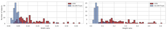
Figure 1.
Distribution of bounding box sizes w.r.t. their image resolution. A comparison between the Online Tracking Benchmark (OTB) [4] in red (ground-level perspective), and the AU-AIR-Track dataset in blue (unmanned aerial vehicle (UAV) perspective). A detailed description of our dataset AU-AIR-Track is given in Section 4.1.
To better deal with the challenges of low-altitude UAV views, we propose a modular detection-by-tracking pipeline coupled with a 3D reconstruction of the environment. The core contributions of this work are as follows: (1) We propose a framework combining three main components. A visual object tracker, for modeling the appearance model of the object and inferring the position of the object in the image. A 3D reconstruction of the static environment, allowing us to associate pixel positions with a corresponding 3D location. Lastly, a state estimator—i.e., particle filter—for estimating the position and velocity of the object in the 3D reconstruction. (2) We show that the incorporation of 3D information into the tracking pipeline has several benefits. A 3D transition model increases the realism of the state estimator predictions, reflecting the corresponding object dynamics. The 3D camera poses allow to compensate for ego-motions, and the depth information improves the handling of object occlusions (see Figure 2). The proposed approach allows us to shift from tracking in 2D image space to tracking in 3D scene space (see Figure 3). (3) We improve the processing of false associations—i.e., distractors—through the usage of a multimodal state estimator. (4) We create a new dataset called AU-AIR-Track, designed for visual object tracking from a UAV perspective. The dataset includes 90 annotated objects as well as annotated occlusions and two 3D reconstructions of the static scenes observed from the UAV. (5) We demonstrate the effectiveness of our pipeline through quantitative results and qualitative analysis.
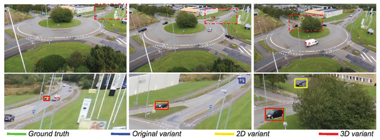
Figure 2.
Qualitative comparison between an original tracking algorithm, its 2D variant, and its 3D variant for UAV onboard visual object tracking. A closer look of the scenario is shown on the lower part of the figure, based on a region delimited by a red dash–dot rectangle in the corresponding upper image. Only the 3D variant is able to overcome the occurring occlusion.
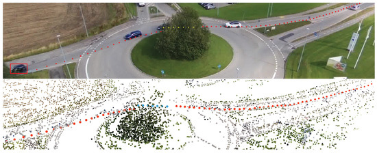
Figure 3.
Qualitative results presenting the trajectory of the object in image space (upper figure) and 3D scene space (lower figure). The red points in both images indicate the 2D and 3D trajectory extracted during tracking. Yellow points (2D) and blue points (3D) indicate the occluded trajectory reconstructed by leveraging a state estimator.
The paper is structured as follows. In Section 2, an overview of related work on single visual object tracking and their corresponding benchmarks is provided. The complete system and the individual components are explained in Section 3. We give a detailed description of the edited dataset used and present metrics with the evaluation protocol for assessing the performance of our approach in Section 4. Finally, in Section 5, we analyze quantitative as well as qualitative results and present the benefits of the design choices made. In the end, we discuss modifications that can be added to our approach in the Section 6 and give a conclusion in Section 7.
2. Related Work
In recent years, great progress regarding single visual object tracking has been made, owing to the abundance of benchmarks available [2,4,5,6,7,8,9,10,11,12,13]. Most of them are designed towards evaluating tracking algorithms on ground-level perspectives, resulting in state-of-the-art visual object trackers following the tracking-by-detection paradigm. Currently, three tracking designs prevail on those benchmarks: the discriminative correlation filters [14,15,16,17,18,19,20]; the Siamese-based approach [21,22,23,24,25,26]; and recently, trackers inspired by correlation filters that employ a small convolutional neural network for learning the appearance model of the object [27,28]. In all three design choices, the main difference lies in how they learn an appearance model of the object. The latter style is explored in this paper.
These tracking algorithms are tailored to scenarios presenting ground-level perspectives, but onboard UAV perspectives present particular challenges. For instance, the object occupies a relatively small portion of the image space, resulting in a less-accurate learned appearance model. This leads to lower discrimination capabilities when similar objects to the tracked object are encountered. In particular, tracking an object with an oblique view on the scene from a UAV can present multiple occlusion situations compared to a top-down view. To analyze the performances of tracking algorithms in UAV scenarios, several benchmarks have been introduced [3,29,30,31], ranging from low to high altitudes, and propose either an oblique view from the UAV or a top-down view. Most participating trackers in the SOT UAV benchmarks use state-of-the-art single visual object trackers presented in ground-level perspective benchmarks without or only with minor adaptations. However, none of the adapted trackers participating in the SOT UAV benchmarks attempt to utilize 3D information. This can be explained by the lack of such information being provided in the datasets. In contrast, the AU-AIR dataset [32] introduced recently is oriented toward object detection from a UAV viewpoint. It offers sequences that capture typical traffic on a roundabout, as would a surveillance drone for traffic monitoring, and contains sequences that are suitable for reconstructing the observed scene in 3D—sufficient translation movements, not flying around excessively, and enough structures in the environment.
In contrast to the SOT UAV benchmark approaches mentioned previously, there are different application domains such as autonomous driving, where objects are tracked in a 3D system of reference through a detection-by-tracking paradigm. Typically, the 2D image detections generated serve as measurements and are mapped from image space in the ego-motion-compensated reference system of the car. An example of applications for traffic monitoring is presented in [33], where the authors propose a pipeline including Multiple Object Tracking (MOT), stereo cues, visual odometry, optical scene flow, and a Kalman filter [34] to enhance tracking performance on the KITTI benchmark [35,36]. A follow up to this study was [37], which reconstructed the static scene and the object in 3D, allowing the shift from tracking in the 2D image space toward tracking in 3D scene space. In addition, the reconstructed object is associated with a velocity, inferred from the optical flow of the object, which is afterward associated with tracklets, thus enabling the authors to tackle occlusion situations and missing detections.
Most related to our work is the approach presented in [38], where the authors developed an MOT pipeline for UAV scenarios that also benefits from a 3D scene reconstruction for estimating the object location in 3D. In contrast to our work, the authors rely on the tracking-by-detection paradigm by leveraging RetinaNet [39] for detecting objects in the image sequence. They generate tracklets on image-level by integrating visual cues and temporal information to reduce false or missing detections. By projecting the image-based positions of detected objects on the estimated ground plane—inferred through visual odometry and multiview-stereo—the framework is able to assess their 3D positions. However, by using an object detector, the authors are only able to track object classes known by the object detector. In contrast, model-free trackers, i.e., SOTs, are able to track arbitrary objects.
We are convinced that tracking applications such as single object visual tracking from a UAV would also benefit from a shift towards a detection-by-tracking paradigm by incorporating 3D information. In this paper, we apply a model-free single object visual tracker, implying that the tracker can only track a single object and starts with a blank appearance model—without an offline/pretrained appearance model. Regardless of the method used for training the tracker—i.e., offline, online—an appearance model of the object is used to locate the object in the image space. Here, we consider the state-of-the-art visual trackers ATOM [27] and DiMP [28] for appearance modeling.
Important for enabling the 2D to 3D mapping is a 3D representation of the observed scene. To this end, a Structure-from-Motion (SfM) or visual Simultaneous Localization and Mapping (SLAM) approach can be leveraged. SfM is a photogrammetric technique that estimates the 3D structures of a scene based on a set of images taken from different viewpoints [40,41,42,43,44,45]. Visual SLAM, similarly to SfM, reconstructs 3D camera poses and scene structures by leveraging specific properties of features in ordered image sets [46,47,48]. In addition, UAVs can improve the robustness of the reconstruction by associating an Inertial Measurement Unit (IMU) with the corresponding SfM or Visual SLAM algorithm [49,50,51,52,53,54,55]. However, in this work, an established software for SfM called COLMAP [40] is used to extract camera poses in the scene space and to reconstruct the static scene.
We estimate the state of the object in 3D space by relying on a state estimator, i.e., a particle filter [56]. For evaluating our approach, the publicly available dataset AU-AIR [32] is employed. The dataset is carefully further edited resulting in the AU-AIR-Track dataset, to best reflect prototypical occlusion situations from a low-altitude oblique UAV perspective.
3. Single Visual Object Tracking Pipeline for UAV
The designed framework is intended to be modular, allowing us to easily substitute different components or add other methods. The essential architecture of our approach is presented in Figure 4.
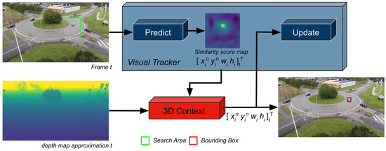
Figure 4.
The architecture of the proposed single visual object tracking framework. The visual tracker outputs a similarity score map inferred in the search area. The similarity score map and depth map approximation corresponding to the image are processed by the 3D Context component, estimating a new position for the object in the image.
On an incoming frame, the visual tracker defines a search area that is based on the previous estimated position and size of the object. The visual tracker then produces a similarity score map along with estimating an initial position and size of the object in the current frame i at time step t. The 3D Context component estimates the location of the object in the 3D scene space through the similarity score map, the depth map approximation, and a state estimator—i.e., a particle filter. This allows the framework to distinguish the object from distractors and also to identify occlusions. Finally, the 3D position estimated by the framework is projected back in the image space as , corresponding to the final estimated position of the object. It should be noted that no semantic information from the scene—i.e., the road—is used to facilitate the tracking process.
Section 3.1 describes the visual tracker component. An overview of the mapping from the 2D image space to the 3D scene space is given in Section 3.2. The particle filter is described in Section 3.3. Lastly, we outline the details of our framework in Section 3.4.
3.1. Visual Appearance Modeling of the Object
In this work, we rely on two state-of-the-art visual trackers, ATOM [27] and DiMP [28]. The chosen trackers achieve top ranks against numerous participants on general visual tracking benchmarks [2,4,6,7,10,12,29]. Figure 5 shows the main components of a standard pipeline for single object tracking, leveraged by methods such as ATOM and DiMP.
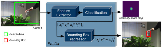
Figure 5.
Block diagram of a visual object tracking pipeline—i.e., ATOM and DiMP—without the update step. During the tracking cycle, salient features from the search area are extracted through a feature extractor. Based on the extracted features, a similarity score map is inferred, used in estimating an initial bounding box of the object. Afterward, a refined bounding box is estimated trough the bounding box regressor, i.e., IoU-Net.
ATOM includes three main components: A (1) Feature Extractor, a pretrained neural network—e.g., ResNet18, ResNet50 [57]—extracting salient features. A (2) Classification component, composed of a two-layer convolutional neural network, which is trained during the tracking process to learn an appearance model of the object. The Classification component proposes an initial estimation of the location and size of the object in the image as a bounding box. Lastly, a (3) Bounding Box regressor component, based on the IoU-Net [58] (trained offline), which refines the initially proposed bounding box.
DiMP is a successor of ATOM and builds on the same elements. The main difference lies in the extension of the Classification component. A new strategy for the initialization of the appearance model is used, expressing the appearance model with better weights at the start. The online learning process for updating the appearance model is also refined for faster and more stable convergence.
For each incoming frame, a search area is created to delimit the possible positions of the object in the frame. The positioning and size of the search area depend on the previous estimated position and size of the object. Based on the features extracted from the search area and the appearance model of the object, a similarity score map is inferred, reflecting the resemblance of the extracted features with the learned appearance model. The highest score in the similarity score map is designated as the position of the object due to the maximum-likelihood approach. The object estimation module—i.e., IoU-Net—is used to identify the best fitting bounding box and thus, to refine the estimated position. To cope with changes in the appearance of the object—e.g., illumination variations, in-plane rotation, motion blur, background clutter—the appearance model of the object has to be adapted during tracking. This adaptation is reached by updating the appearance model regularly in ATOM and DiMP. The updates occur every 10 valid frames for ATOM and every 15 valid frames for DiMP. A valid frame corresponding to a frame where the object has been identified correctly—with a high similarity score. The new appearance model is adapted by retraining the classification component with the search areas of those valid frames. The tracker deals with distractors by recognizing multiple peaks in the similarity score map and immediately updating the appearance model of the object with a high learning rate.
3.2. Point Cloud Reconstruction of the Environment
We employ Structure-from-Motion (SfM) for achieving the mapping between the 2D image space and the 3D reference system, i.e., scene space. Owing to our modular design, the mapping between the 2D image space and the 3D scene space can be replaced with an alternative photogrammetric technique. For this paper, we create a point cloud representation of the observed environment, which is sufficient for the demonstration of our approach.
We leverage COLMAP (in our experiments we used COLMAP 3.6, available publicly under https://colmap.github.io/ (accessed on 14 October 2020)) [40,59], which is an established approach for SfM. For a given image set that contains overlapping images of the same scene and taken from different viewpoints, COLMAP automatically extracts the corresponding camera poses and reconstructs the scene structures in 3D. To achieve this, the library follows common SfM steps. (1) A correspondence search, where salient features from an image set are extracted and matched across the images, and incorrectly matched features are filtered out. (2) The scene is reconstructed as a point cloud by performing image registration, feature triangulation, and bundle adjustments.
Figure 6a presents a point cloud reconstruction leveraged by COLMAP on an image sequence of AU-AIR-Track. The initial reconstruction of the scene contains noise near the camera frame and statistical outliers. Points near the camera frame are falsely triangulated and outliers are points correctly positioned but that are too sparse for reliably representing structures of the scene. To reduce the number of incorrect points in the reconstruction, we filter out points close to the camera frame and statistical outliers. We discard near-camera points from the point cloud by comparing their Euclidean distance with a threshold. For statistical outliers, we proceed as follows: (1) We define a neighborhood of 10 neighbors. The average distance of a given point i to its neighbors is calculated using the Euclidean distance. (2) A standard deviation threshold is defined and the overall average for all is computed as . Points with an average distance are identified as outliers and discarded from the point cloud. Figure 6b,c display the removal of points close to the camera frame and statistical outliers. Moreover, a plane ground is estimated by using the Random sample consensus (RANSAC) [60] method (see Figure 7). Points below the ground plane are discarded.
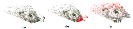
Figure 6.
(a) A point cloud reconstruction using COLMAP. (b) Highlighted noise near the frame of reference in red. (c) Highlighted outliers in red after removing near-frame reference noise.
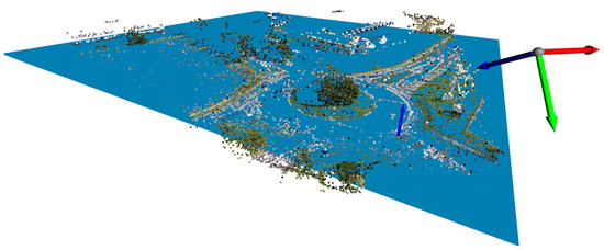
Figure 7.
A filtered point cloud with the corresponding ground plane in blue.
We compute depth map approximations based on the new scene reconstructed, i.e., the filtered point cloud with the estimated ground plane. The depth map approximations encode, for every pixel, the distance between the positions of the UAV and the visible points in the scene for the corresponding viewpoint, i.e., camera pose. For every frame in the AU-AIR-Track dataset, a corresponding depth map approximation is constructed by relying on the pinhole camera model; thus, enabling the mapping between the 2D image space and the 3D scene space. Figure 8 displays a depth map approximation example with the corresponding frame.
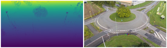
Figure 8.
Comparison between a depth map approximation (left) and the corresponding frame (right). Points in yellow on the frame indicate visible points from the point cloud reconstruction aside from the ground estimation.
3.3. Particle Filter for Modeling the Object in 3D
In order to overcome the drawbacks of the common maximum-likelihood approach used in SOTs, we switch to detection-by-tracking by applying an additional state estimator. Additionally, to robustly handle multiple high similarity scores in the similarity score map, a state estimator with a multimodal representation of the probability density function is favored. To that end, a particle filter [56] is used, which will estimate the state of the object—i.e., the position and velocity—in the 3D scene for every time step t. The particle filter estimates the posterior density function of the object based on a transition model f, the current observation , and the prior density function . The general idea is shown in Equation (1):
In order to approximate the probability density function , the particle filter uses particles. Each particle denotes a hypothesis on the state. Particles from the prior probability density function are propagated through the transition model f. Weights at time step t are assigned to n particles with , mirroring how strongly particles match with the current observation . Let represent the probability density function of the posterior state given all observations up to time step t in Equation (2). Each particle has a corresponding weight at time step t. Let denote the hypothesis on the state of the i-th particle and the state estimation at time t. is the Dirac delta function. The weights are normalized such that . Particles are weighted according to their matching similarity with the current observation .
A resampling is performed after the weighting of the particles whenever , presented in Equation (3), is below a certain threshold. The resampling allows the particle filter to discard low-weighted particles and create new particles based on the stronger-weighted ones, allowing a refined approximation of .
In our case, the observation is the similarity score map produced by ATOM or DiMP. We apply a constant velocity model for the transition model f and fix the velocity on the axis, as —where is perpendicular to the estimated ground plane of the reconstructed scene. This results in particles being only able to move on the ground.
3.4. Tracking Cycle and Occlusion Handling
During initialization, the visual tracker learns an appearance model of the object based on the initial bounding box. At the same time, the position of the object in the image is projected onto the estimated ground plane of the 3D reconstruction, i.e., the scene space. To this end, we rely on the pinhole camera model for estimating the depth value of the object in the scene space. Supposing that the object does not leave the ground in the real world, we can assume that the object is bound to only move on the plane ground . Let describe the normal vector of the plane ground and describe the position of the object on the plane—expressed in camera frame coordinates. In Equation (4), we describe the plane in standard form for a generic point on the plane. In Equation (5), we define and , where are the image coordinates of the object inferred by the visual tracker and f is the focal length of the camera. By replacing and in Equation (4) and simplifying it, we obtain Equation (6), allowing us to infer the depth value for the object based on its image coordinates . Now that the depth value is estimated, we can determine the missing coordinates and of based on Equation (5). By applying a rigid body transformation from the camera to the world frame of reference, we obtain the position of the object in the scene space as .
The projected position for the first frame , expressed in 3D coordinates, is considered as the initial position for the state . In the following frame, the visual tracker component computes a bounding box delimiting the position and size of the object in the frame. Additionally, we extract the current search area and the similarity score map. Particles are generated uniformly onto the ground of the 3D reconstruction but are delimited on the projected surface of the search area. Particles are then weighted accordingly to the similarity score map of the visual tracker component. Following is a resampling step, which shrinks the possible locations where the object might be located by regenerating new particles where previous high-weighted particles were located. In consequence, particles are mostly located around a high similarity response, giving us an estimated position of the object in 3D. The current 3D position along with the previous 3D position of state are used to determine an initial velocity. As a result, an initial state for the object is estimated with velocity and position.
In the following frame, the particle filter can be used to predict the position of the object in the scene space as . To deal with the uncertainties in the transition model—i.e., the constant velocity model—a Gaussian noise term is added along and .
After initialization, our tracking framework enters an online tracking cycle. Figure 4 presents the essential architecture of the framework during online tracking. On an incoming frame, the visual tracker component defines a search area and produces a similarity score map along with estimating a bounding box for the object on frame t. During the 3D Context computation step, we estimate the 3D position of the object in the scene space, distinguish the object from distractors, and recognize occlusions. The new 3D position of the object expressed in the scene space is projected back onto the frame t, corresponding to the new estimated position of the object in image space. Figure 9 displays the different building blocks of the 3D Context component, which contains the particle filter that estimates the object state, i.e., the 3D position and 3D velocity in the scene space. In the first step, the particle filter predicts particles on an incoming frame. The predicted particles are clustered in the image space. We then identify the cluster representing the object based on how close each cluster is to the previously estimated position of the object in the scene space.
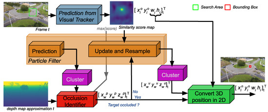
Figure 9.
Detailed view of the architecture with the Context 3D component. The prediction of the particle filter and the depth map approximation are used to identify occluded particles. Particles are clustered depending on their position in the image to identify potential groups, such as the object and distractors. In case the object is considered as occluded, the 3D coordinate of the prediction provided by the particle filter is used as the presumed position of the object in the scene space and is reprojected in the image as . In case the object is not identified as occluded, an update and resampling are performed on the particles before clustering them for a second time. Following is the determination of the cluster representing the object. Lastly, the 3D coordinates of the cluster, modeling the object in the scene space, are reprojected in the image as .
The occlusion identifier component identifies occluded particles composing the object cluster through the depth map approximation. To this end, we compare the depth value of the predicted particles from the perspective of the UAV and the depth value from the depth map approximation. We identify particles hidden by structures if there is a discrepancy between the predicted depth and the observed depth. We considered that if 50% of the particles from the object cluster are occluded, then the object is also occluded. Similarly, the object is automatically considered as hidden if the similarity score map is flat and widely spread over the search area. Should the object be identified as occluded, the tracking framework would rely on the predictions provided by the particle filter .
To identify the reappearance of the object, a high similarity score close to the expected position is required. When more than 50% of the predicted particles are not labeled as occluded, we consider that the object is potentially visible again. A specific threshold for the similarity score map is set to consider the object as being truly visible again. A similarity score greater-than or equal-to this threshold must be reached to consider updating the particle filter with the observation, i.e., the similarity score map. If distractors are present when the object reappears, then the group of particles closest to the prediction is considered to represent the object.
When the object is visible, a second step is to update the belief of the particle filter with the observation, i.e., similarity score map. However, before updating a small percentage, i.e., 10%, of particles are uniformly redistributed across the projected search area on the ground. This redistribution ensures that we maintain a multimodal distribution. Without redistributing a portion of the particles, particles would clump around the object and only a small portion of the similarity score map would be considered for updating the weights. The weights of the particles are updated by projecting their 3D position in the image space, allowing us to weigh them accordingly to their 2D location in the similarity score map. We then resample particles through stratified resampling [61]. By using a particle filter, we can model multimodal tracking, preventing instantaneous switching from object to distractors as illustrated in Figure 10.
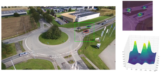
Figure 10.
The small green bounding box represents the estimated bounding box of the unmodified visual object tracker and the red bounding box represents the estimated bounding box of a visual object tracker coupled with a particle filter. The large green bounding box corresponds to the search area of the visual tracker. In this scenario, the similarity score map has three peaks. Due to the maximum-likelihood approach of the visual tracker, it mistakes a distractor with the object; whereas the visual tracker coupled with a particle filter manages to stay on the object, even though the highest similarity score is attached to a distractor.
After particles are resampled, the framework clusters them based on their position in the image space. We identify the cluster describing the object, by comparing the position for every cluster c against the predicted position of the object . The closest cluster to the predicted position is considered to describe the object state. Thus, the new/updated position of the object is based on this identified cluster as . The coordinates in the scene space are then projected in the image space as and used for updating the appearance model of the visual tracker component. This avoids adding incorrect training samples, i.e., distractors.
4. Dataset and Evaluation Metrics
In Section 4.1, we present our edited AU-AIR-Track dataset. In Section 4.2, we define the metrics used for evaluating the trackers on the dataset.
4.1. AU-AIR-Track Dataset
Using our approach, we want to tackle occlusion occurrences, false associations, and ego-motion using a 3D reconstruction of the static scene. To that end, we need a UAV dataset that provides visual object tracking annotations with 3D reconstructions of the scene. As stated before, current UAV datasets [3,29,30,31] with visual tracking annotations do not provide 3D information. Therefore, we created the AU-AIR-Track dataset (AU-AIR-Track alongside AU-AIR [32] are available under https://github.com/bozcani/auairdataset (accessed on 14 October 2020)) which includes the following: bounding box annotations with identification numbers, occlusion annotations, 3D reconstructions of the scene with the corresponding depth map approximations, and camera poses.
AU-AIR-Track is distilled from the AU-AIR dataset [32], which provides real-world sequences suitable for traffic surveillance and reflects prototypical outdoor situations captured from a UAV. AU-AIR contains sequences taken from a low flight altitude ranging from 10 to 30 m, under different camera angles ranging from approximately 45 to 90 degrees. For each frame, the dataset provides recording time stamps, Global Positioning System (GPS) coordinates, altitude information, IMU data, and the velocity of the UAV. A criterion in favor of AU-AIR is the low range altitude flights with the oblique point of view towards the scene it provides, the multiple occlusions offered by the tree in the roundabout and the duration of a scene is observed.
The AU-AIR-Track dataset consists of two sequences, designated as 0 and 1. With a total of 90 annotated objects, sequence 0 contains 887 frames and 63 annotated objects; and sequence 1 has 512 frames with 27 annotated objects. Both sequences have been extracted at 5 frames per second and their resolution is 1920 × 1080 and 1922 × 1079 pixels, respectively. Figure 11 and Figure 12 display a few images from both sequences, which present only oblique views of the scene taken from a nonstationary UAV.
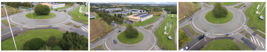
Figure 11.
Examples of images from sequence 0 of AU-AIR-track.
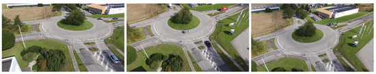
Figure 12.
Examples of images from sequence 1 of AU-AIR-track.
As a result, the main challenges captured in AU-AIR-Track are the constant camera motion, the low image resolution, the presence of distractors, and most importantly, frequent object occlusions. Since AU-AIR annotations are designed for object detection, we adapted them in AU-AIR-Track for visual object tracking. Figure 13 presents the original AU-AIR annotations and the adapted annotations for AU-AIR-Track (where only moving objects are annotated).
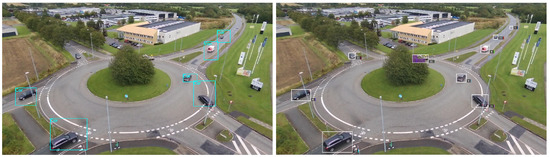
Figure 13.
Comparison between original annotation from AU-AIR (left) and adapted annotations for visual object tracking (right). Purple color indicates that a region of the bounding box is occluded.
Figure 14 shows the distribution of the ground-truth bounding box locations for both sequences. The value of each pixel denotes the probability of a bounding box to cover that pixel over an entire sequence. It can be seen that most objects follow the underlying scene structure, i.e., the road. From the 63 possible objects present in sequence 0, 45 objects undergo an occlusion and 25 out of 27 objects in sequence 1. As stated before, AU-AIR-Track provides the 3D reconstructions of both sequences (see Figure 15). The 3D information available in our dataset are the sparse reconstructions with their respective ground plane estimations, camera poses, fundamental matrices, and transformation matrices.
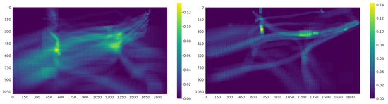
Figure 14.
The probability distribution of ground-truth bounding boxes over the total sequence length for sequence 0 (left) and sequence 1 (right) from AU-AIR-Track.
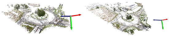
Figure 15.
Filtered point cloud for both sequences composing the dataset. Left is a reconstruction of sequence 0 and right of sequence 1.
4.2. Evaluation Metrics
Similar to long-term tracking, the tracked object can disappear and reappear. Thus, no manual reinitialization is done when the tracker loses the object. To measure the performance, we utilize common long-term metrics—tracking precision , tracking recall , and tracking F1-score —at a given , introduced in [62] and used in [2,6].
Let be the ground truth object bounding box, and the bounding box estimation given by the tracker at frame t. Further, let denote the prediction confidence, which in our case, is the maximal score given by the tracker regarding its confidence on the presence of the object in the current frame t. If the object is partially/fully occluded, we set ; and similarly, if the trackers predicts an object with a confidence below , we set . Furthermore, let denote the number of frames with , where , is the number of frames with , and with . Lastly, describes the intersection-over-union (IoU) between and .
The combination of tracking precision and tracking recall as a single score is defined as the tracking F1-score [62]. Similarly to the long term challenges presented in [2,6], the final tracking F1-score is used to rank the different tracking algorithms.
The evaluation protocol is as follows: the trackers are evaluated on all objects present in the AU-AIR-Track. The annotated first frame of the object is used to initialize the tracker. From there, the tracker outputs a prediction bounding box for every subsequent frame where the object is annotated—even during occlusions, no reset is allowed. Tracking precision, tracking recall, and tracking F1-score are computed accordingly to Equations (7)–(9). To avoid statistical errors caused by the classification component of the visual tracker, which describes the appearance of the object through learned weights, we run an evaluation of every tracker five times on both sequences of the AU-AIR-Track. For every evaluation e and for every object i present in a sequence, we take the maximum tracking F1-score for that object . Considering the maximum tracking F1-score, regardless of , allows us to examine how the tracker would work without human intervention.
For computing the final F1-score of a tracker on a sequence of AU-AIR-Track: (1) we average maximum tracking F1-scores extracted from different evaluations e for the same object i; then, (2) we average all belonging to the same sequence. Equation (10) describes how we computed . Let i denote the index of the object, with ; and let e describe the index for an evaluation, where . In our case, we performed five evaluations for each tracker on the AU-AIR-Track.
5. Results
In this section, we demonstrate the effectiveness of our approach on quantitative results in Section 5.1 and through a qualitative analysis in Section 5.2.
5.1. Quantitative Results
In this section, we use the following terms: (1) “original”, which refers to the unmodified visual object tracker ATOM and DiMP presented in [27,28]. (2) ”2D variant“, denoting ATOM and DiMP—i.e., ATOM-2D, DiMP-2D—coupled with a particle filter, working in the 2D image space. (3) Lastly, the “3D variant” refers to ATOM and DiMP—i.e., ATOM-3D, DiMP-3D—utilizing 3D information combined with a particle filter operating in this 3D scene space. Table 1 summarizes the final tracking F1-scores of ATOM and DiMP for every variation. Best on each sequence and for each variant are indicated in bold.

Table 1.
Final tracking F1-scores and standard deviation for every tracker variation evaluated on AU-AIR-Track.
Based on Table 1, we observe that the original variations of ATOM and DiMP attain the lowest scores and the least stable results. As stated before, the original methods are designed for short-term tracking from a ground-level perspective by relying on visual cues. The original variants have no specific module integrated for handling partial or full occlusions apart from using a similarity score map with a threshold. If the similarity score map has no peaks (under a set threshold) and is widely spread, the tracker is able to recognize that the object is missing but is not able to predict the next position. The original variation is also more prone to switching the object with a false association—i.e., the distractor—because of the maximum-likelihood approach. Since the original trackers rely only on the learned appearance model, they are extremely dependent on the number of pixels that encode the object. This results in the tracker losing most of the tracked object when they are described with a low amount of pixels, i.e., small-scale objects.
ATOM-2D and DiMP-2D also recognize occlusion only through visual cues, achieved by setting a minimum required similarity score as a threshold. Occlusion is identified by obtaining a similarity score that is below the set threshold. During occlusion, the position of the object cannot be inferred visually but can be estimated (to some extent) through the predictions of the particle filter. Relying solely on visual cues for identifying occlusion is limited since the tracker potentially misinterprets a fast appearance change with an occlusion. Another limitation is that only occlusions without ego-motion can be handled because the particle filter estimates positions in the 2D image space. Overall, there is an increase in the tracking F1-score compared to the original variations, but this gain is essentially due to better recognizing and handling of distractors and small-scale objects, leveraged by a multimodal state estimator. With the multimodal property, we allow groups of particles to form where high responses in the similarity score map are found. The different groups of particles are clustered depending on their locations, enabling the 2D trackers to consider and distinguish the object and distractors. Whereas, the original trackers, utilizing a maximum-likelihood approach, can only handle the highest response in the similarity score map. Using a state estimator also offers the benefit of being less dependent on the number of pixels used for encoding the object.
Regarding ATOM-3D and DiMP-3D, this variation achieves the best performance on the AU-AIR-Track dataset. ATOM-3D and DiMP-3D can identify occlusions not only based on visual cues but also through depth information leveraged by the 3D reconstruction of the scene (depth map approximations). This allows them to recognize a hidden object more reliably than the previous variations. Using a particle filter in the 3D scene space enables the usage of a 3D transition model, which adequately describes real-world motions in comparison to a particle filter in 2D image space. This results in improved stability of corresponding predictions w.r.t. ego-motions. Thus, the predictions of the state estimator are more accurate than in the 2D variants when the object is hidden, allowing them to potentially estimate the position of the object for a longer period. Additionally, in this variation, the particle filter enhances the ability (similarly to ATOM-2D and DiMP-2D) of the tracker to distinguish the objects from distractors and to be less dependent on the number of pixels describing the object. Based on these results, the ATOM-3D and DiMP-3D display better performance in comparison to the original and 2D variants.
5.2. Qualitative Analysis
In this section, we discuss selected qualitative tracking scenarios to verify the overall viability of the different methods. To illustrate the results, an in-depth look is provided by examining the variants of DiMP. For every figure, a closer look at the scenario is shown on the lower part of the figure, based on a region delimited by a red dash–dot rectangle in the corresponding upper image.
Figure 16 and Figure 17 display scenarios where the object is lost by the original DiMP variant in contrast to DiMP-2D and DiMP-3D. In the first scenario, the original variant, which uses a maximum-likelihood approach, misinterprets the distractor with the object because of the low number of pixels encoding the object. In contrast, by leveraging a particle filter, DiMP-2D and DiMP-3D handle the presence of distractors better and are less prone to fail on small-scale objects. The second scenario presents an occlusion situation, where the object is hidden by the tree in the roundabout. Both DiMP-2D and DiMP-3D recognize occlusion and can rely on their respective particle filter for predicting the position of the hidden object, until its reappearance.
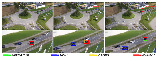
Figure 16.
Comparison of the evaluated trackers. DiMP-2D and DiMP-3D are able handle the presence of a distractors by taking advantage of the multimodal representation provided by a particle filter. In contrast, using the maximum-likelihood approaches, DiMP switches to a distractor.
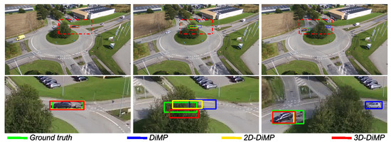
Figure 17.
Comparison between the three DiMP variations. In this scenario, the 2D- and 3D-DiMP methods can handle the object undergoing occlusion.
Figure 18 shows three consecutive frames where only DiMP-3D is unaffected by the ego-motion and can track the object robustly because the position of the object is expressed in the 3D scene space. Figure 19 illustrates another scenario where both DiMP-2D and DiMP-3D recognize the object as hidden, but while predicting the position of the hidden object; only DiMP-3D can predict robust and reasonable positions for the object even during camera motion. Relying on an image-based state estimator is only viable when ego-motion is very minimal, as in Figure 17. In Figure 20, solely DiMP-3D can identify the object undergoing occlusion, owing to the depth information leveraged by the depth map approximations in addition to the visual cues; whereas DiMP and DiMP-2D switch to a distractor because they solely rely on visual cues.
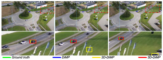
Figure 18.
Comparison between DiMP-2D and DiMP-3D. During camera motion DiMP-2D is unable to track the object; whereas DiMP-3D is able to stabilize the tracking by expressing the object position in the 3D scene space. The light-blue grid is drawn to help visualize ego-motion.
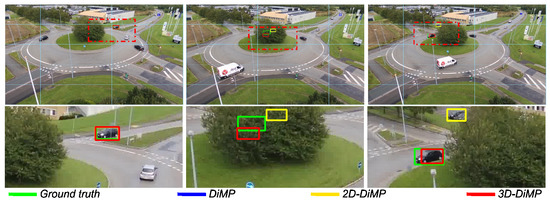
Figure 19.
Comparison between DiMP-2D and DiMP-3D. Only DiMP-3D is able to robustly track the object during ego-motion while the object is occluded. The light-blue grid is drawn to help visualize ego-motion.
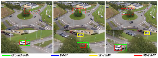
Figure 20.
Comparison between DiMP variations. Owing to the depth information used for occlusion identification in addition to visual cues, DiMP-3D manages to handle the object undergoing occlusion; whereas DiMP and DiMP-2D switch to a distractor caused by relying solely on visual cues.
Despite DiMP-3D and ATOM-3D achieving remarkable results, there are cases where both fail. Occlusion on rare occasions is not identified correctly because of a strong distractor present when the object is partially hidden. This can be prevented by elaborating a different strategy for recognizing occlusions and reappearances of the object. Another point limiting the performance of DiMP-3D is illustrated in Figure 21, where the object slows down at the intersection for a long period. While the object is not moving, the particle filter continuously updates the estimated velocity to be adequate with the observations (velocity near zero). When the object accelerates, the particle filter cannot match the speed instantly, due to the transition model.
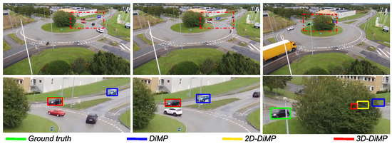
Figure 21.
Comparison between DiMP-2D and DiMP-3D. During the acceleration phase of the object, the particle filter estimates the velocity of the object with a delay due to the transition model adopted.
6. Discussion
Besides the challenges arising from the specific characteristics for single visual object tracking from UAVs, the use of computer vision approaches onboard a UAV additionally faces the problem of finding an adequate compromise between computational complexity and real-time capabilities with extreme resource limitations on the platform. Although, being not in the scope of this paper, we explore in this section alternative design choices for integrating the current pipeline onto a UAV. Owing to the modular design of our pipeline, we can replace individual components with variants that are less cost-intensive.
Regarding the Visual Object Tracker component, both ATOM [27] and DiMP [28] have real-time capabilities but rely on a Graphics Processing Unit (GPU) for inferring the position of the object. To diminish the amount of space required and to increase the run time, the original feature extractor—i.e., ResNet-18, ResNet-50 [57]—could be replaced with MobileNet [63], which is specifically designed for embedded vision applications and mobile devices. Alternatively, it is possible to replace ATOM and DiMP with another type of tracker. Since both trackers update the appearance model of the object on-the-fly, they require more GPU capacities than other methods not updating the appearance model such as Siamese SOT [21,23,24,25].
In our work, we focused on using image-based scene reconstruction by leveraging a SfM-based method [40]. To attain real-time performance, a Visual SLAM-based method that can associate IMU formations [49,50,51,52,53,54,55] is preferred for robustly reconstructing the 3D environment on-the-fly. A concern for the sparse reconstruction might be the storage and the processing time needed when the UAV is observing a large area. To reduce the required storage space needed, the point cloud can be reconstructed or partially loaded, depending on the current UAV position in the scene [64].
Since the multimodal representation of the probability density function is indispensable, for identifying distractors in the search area, a particle filter [56] is utilized in our detection-by-tracking pipeline. Thus, using a particle filter over other state estimators such as the Kalman filter [34] is crucial for the proposed pipeline, despite being computationally more demanding. Although numerous particle filter implementations do not perform well with a high number of particles, this is not necessarily a general limitation of the approach [65]. In an effort to reduce the computational time, authors from [66] elaborate faster methods for the resampling step compared to common resampling approaches.
7. Conclusions
In this paper, we propose an approach to improve UAV onboard single visual object tracking. To this end, we combine information extracted from a visual tracker and 3D cues of the observed scene. The 3D reconstruction allows us to estimate the state in a 3D scene space rather than in a 2D image space. Therefore, we can define a 3D transition model reflecting the dynamics of the object close to reality.
The potential of the approach is shown on challenging real-world sequences, illustrating typical occlusion situations captured from a low-altitude UAV. The experiments demonstrate that the presented framework has several advantages and is viable for UAV onboard visual object tracking. We can effectively handle object occlusions, low object sizes, the presence of distractors, and reduced tracking errors caused by ego-motion.
A part of our future work will be to exploit a dense reconstruction rather than a sparse reconstruction; explore different state estimators and add more context to the scene, such as the layout of the road in the reconstruction; and to integrate real-world coordinates through georeferencing.
Author Contributions
Conceptualization by the first author S.V. and the co-authors S.B. (Stefan Becker) and T.B. Data curation, formal analysis, investigation, methodology, software, validation, visualization, and writing—original draft, were done by the first author S.V. The co-authors S.B. (Stefan Becker) and S.B. (Sebastian Bullinger) improved the paper through their comments and corrections about the layout, content, and the obtained results. Supervision and project administration were done by N.S.-N. Funding acquisition was done by M.A. All authors have read and agreed to the published version of the manuscript.
Funding
This research was funded by the German Ministry of Defence.
Acknowledgments
We would like to thank Ann-Kristin Grosselfinger, who provided the annotations for the AU-AIR-Track dataset.
Conflicts of Interest
The authors declare no conflict of interest.
Abbreviations
The following abbreviations are used in this manuscript:
| UAV | Unmanned Aerial Vehicle |
| SOT | Single Object Tracking |
| MOT | Multiple Object Tracking |
| SfM | Structure from Motion |
| SLAM | Simultaneous Localization and Mapping |
| IMU | Inertial Measurement Unit |
| RANSAC | Random Sample Consensus |
| GPS | Global Positioning System |
| IoU | Intersection-over-Union |
| GPU | Graphics Processing Unit |
References
- Black, J.; Ellis, T.; Rosin, P. A novel method for video tracking performance evaluation. In Proceedings of the IEEE International Workshop on Visual Surveillance and Performance Evaluation of Tracking and Surveillance (VS-PETS 03), Beijing, China, 11–12 October 2003; pp. 125–132. [Google Scholar]
- Kristan, M.; Matas, J.; Leonardis, A.; Felsberg, M.; Pflugfelder, R.; Kamarainen, J.K.; Cehovin Zajc, L.; Drbohlav, O.; Lukezic, A.; Berg, A.; et al. The seventh visual object tracking VOT2019 challenge results. In Proceedings of the IEEE International Conference on Computer Vision Workshops, Seoul, Korea, 27 October–2 November 2019. [Google Scholar]
- Zhu, P.; Wen, L.; Du, D.; Bian, X.; Hu, Q.; Ling, H. Vision Meets Drones: Past, Present and Future. arXiv 2020, arXiv:2001.06303. [Google Scholar]
- Wu, Y.; Lim, J.; Yang, M.H. Object tracking benchmark. IEEE Trans. Pattern Anal. Mach. Intell. 2015, 37, 1834–1848. [Google Scholar] [CrossRef] [PubMed]
- Wu, Y.; Lim, J.; Yang, M.H. Online Object Tracking: A Benchmark. In Proceedings of the IEEE Conference on Computer Vision and Pattern Recognition (CVPR), Portland, OR, USA, 23–28 June 2013. [Google Scholar]
- Kristan, M.; Leonardis, A.; Matas, J.; Felsberg, M.; Pflugfelder, R.; Cehovin Zajc, L.; Vojir, T.; Bhat, G.; Lukezic, A.; Eldesokey, A.; et al. The sixth visual object tracking VOT2018 challenge results. In Proceedings of the European Conference on Computer Vision (ECCV), Munich, Germany, 8–14 September 2018. [Google Scholar]
- Fan, H.; Lin, L.; Yang, F.; Chu, P.; Deng, G.; Yu, S.; Bai, H.; Xu, Y.; Liao, C.; Ling, H. LaSOT: A High-Quality Benchmark for Large-Scale Single Object Tracking. In Proceedings of the IEEE Conference on Computer Vision and Pattern Recognition (CVPR), Long Beach, CA, USA, 16–20 June 2019. [Google Scholar]
- Smeulders, A.W.; Chu, D.M.; Cucchiara, R.; Calderara, S.; Dehghan, A.; Shah, M. Visual tracking: An experimental survey. IEEE Trans. Pattern Anal. Mach. Intell. 2013, 36, 1442–1468. [Google Scholar]
- Valmadre, J.; Bertinetto, L.; Henriques, J.F.; Tao, R.; Vedaldi, A.; Smeulders, A.W.; Torr, P.H.; Gavves, E. Long-term Tracking in the Wild: A Benchmark. In Proceedings of the European Conference on Computer Vision (ECCV), Munich, Germany, 8–14 September 2018. [Google Scholar]
- Huang, L.; Zhao, X.; Huang, K. GOT-10k: A Large High-Diversity Benchmark for Generic Object Tracking in the Wild. IEEE Trans. Pattern Anal. Mach. Intell. 2019. [Google Scholar] [CrossRef] [PubMed]
- Liang, P.; Blasch, E.; Ling, H. Encoding Color Information for Visual Tracking: Algorithms and Benchmark. IEEE Trans. Image Process. 2015, 24, 5630–5644. [Google Scholar] [CrossRef] [PubMed]
- Muller, M.; Bibi, A.; Giancola, S.; Alsubaihi, S.; Ghanem, B. TrackingNet: A Large-Scale Dataset and Benchmark for Object Tracking in the Wild. In Proceedings of the European Conference on Computer Vision (ECCV), Munich, Germany, 8–14 September 2018. [Google Scholar]
- Li, A.; Chen, Z.; Wang, Y. BUAA-PRO: A Tracking Dataset with Pixel-Level Annotation. In Proceedings of the BMVC, Newcastle, UK, 3–6 September 2018; p. 249. [Google Scholar]
- Bolme, D.S.; Beveridge, J.R.; Draper, B.A.; Lui, Y.M. Visual object tracking using adaptive correlation filters. In Proceedings of the 2010 IEEE Computer Society Conference on Computer Vision and Pattern Recognition, San Francisco, CA, USA, 13–18 June 2010; IEEE: Piscataway, NJ, USA, 2010; pp. 2544–2550. [Google Scholar]
- Danelljan, M.; Hager, G.; Shahbaz Khan, F.; Felsberg, M. Learning spatially regularized correlation filters for visual tracking. In Proceedings of the IEEE International Conference on Computer Vision, Santiago, Chile, 7–13 December 2015; pp. 4310–4318. [Google Scholar]
- Danelljan, M.; Robinson, A.; Khan, F.S.; Felsberg, M. Beyond correlation filters: Learning continuous convolution operators for visual tracking. In European Conference on Computer Vision; Springer: Berlin/Heidelberg, Germany, 2016; pp. 472–488. [Google Scholar]
- Kiani Galoogahi, H.; Sim, T.; Lucey, S. Correlation filters with limited boundaries. In Proceedings of the IEEE Conference on Computer Vision and Pattern Recognition, Boston, MA, USA, 7–12 June 2015; pp. 4630–4638. [Google Scholar]
- Henriques, J.F.; Caseiro, R.; Martins, P.; Batista, J. High-speed tracking with kernelized correlation filters. IEEE Trans. Pattern Anal. Mach. Intell. 2014, 37, 583–596. [Google Scholar] [CrossRef] [PubMed]
- Ma, C.; Huang, J.B.; Yang, X.; Yang, M.H. Hierarchical convolutional features for visual tracking. In Proceedings of the IEEE International Conference on Computer Vision, Santiago, Chile, 7–13 December 2015; pp. 3074–3082. [Google Scholar]
- Sun, C.; Wang, D.; Lu, H.; Yang, M.H. Correlation tracking via joint discrimination and reliability learning. In Proceedings of the IEEE Conference on Computer Vision and Pattern Recognition, Salt Lake City, UT, USA, 18–22 June 2018; pp. 489–497. [Google Scholar]
- Bertinetto, L.; Valmadre, J.; Henriques, J.F.; Vedaldi, A.; Torr, P.H. Fully-convolutional siamese networks for object tracking. In European Conference on Computer Vision; Springer: Berlin/Heidelberg, Germany, 2016; pp. 850–865. [Google Scholar]
- Guo, Q.; Feng, W.; Zhou, C.; Huang, R.; Wan, L.; Wang, S. Learning dynamic siamese network for visual object tracking. In Proceedings of the IEEE International Conference on Computer Vision, Venice, Italy, 22–29 October 2017; pp. 1763–1771. [Google Scholar]
- Li, B.; Wu, W.; Wang, Q.; Zhang, F.; Xing, J.; Yan, J. Siamrpn++: Evolution of siamese visual tracking with very deep networks. In Proceedings of the IEEE Conference on Computer Vision and Pattern Recognition (CVPR), Long Beach, CA, USA, 16–20 June 2019. [Google Scholar]
- Li, B.; Yan, J.; Wu, W.; Zhu, Z.; Hu, X. High performance visual tracking with siamese region proposal network. In Proceedings of the IEEE Conference on Computer Vision and Pattern Recognition, Salt Lake City, UT, USA, 18–22 June 2018; pp. 8971–8980. [Google Scholar]
- Wang, Q.; Teng, Z.; Xing, J.; Gao, J.; Hu, W.; Maybank, S. Learning attentions: Residual attentional siamese network for high performance online visual tracking. In Proceedings of the IEEE Conference on Computer Vision and Pattern Recognition, Salt Lake City, UT, USA, 18–22 June 2018; pp. 4854–4863. [Google Scholar]
- Zhang, L.; Gonzalez-Garcia, A.; Weijer, J.v.d.; Danelljan, M.; Khan, F.S. Learning the model update for siamese trackers. In Proceedings of the IEEE International Conference on Computer Vision, Seoul, Korea, 27 October–2 November 2019; pp. 4010–4019. [Google Scholar]
- Danelljan, M.; Bhat, G.; Khan, F.S.; Felsberg, M. ATOM: Accurate Tracking by Overlap Maximization. In Proceedings of the IEEE Conference on Computer Vision and Pattern Recognition (CVPR), Long Beach, CA, USA, 16–20 June 2019. [Google Scholar]
- Bhat, G.; Danelljan, M.; Gool, L.V.; Timofte, R. Learning discriminative model prediction for tracking. In Proceedings of the IEEE International Conference on Computer Vision, Seoul, Korea, 27 October–2 November 2019; pp. 6182–6191. [Google Scholar]
- Mueller, M.; Smith, N.; Ghanem, B. A benchmark and simulator for uav tracking. In European Conference on Computer Vision; Springer: Berlin/Heidelberg, Germany, 2016; pp. 445–461. [Google Scholar]
- Li, S.; Yeung, D.Y. Visual object tracking for unmanned aerial vehicles: A benchmark and new motion models. In Proceedings of the AAAI, San Francisco, CA, USA, 4–7 February 2017. [Google Scholar]
- Du, D.; Qi, Y.; Yu, H.; Yang, Y.; Duan, K.; Li, G.; Zhang, W.; Huang, Q.; Tian, Q. The unmanned aerial vehicle benchmark: Object detection and tracking. In Proceedings of the European Conference on Computer Vision (ECCV), Munich, Germany, 8–14 September 2018; pp. 370–386. [Google Scholar]
- Bozcan, I.; Kayacan, E. AU-AIR: A Multi-modal Unmanned Aerial Vehicle Dataset for Low Altitude Traffic Surveillance. In Proceedings of the 2020 IEEE International Conference on Robotics and Automation (ICRA), Paris, France, 31 May–31 August 2020. [Google Scholar]
- Ošep, A.; Mehner, W.; Mathias, M.; Leibe, B. Combined Image- and World-Space Tracking in Traffic Scenes. In Proceedings of the ICRA, Singapore, 29 May–3 June 2017. [Google Scholar]
- Welch, G.; Bishop, G. An Introduction to the Kalman Filter. 1995. Available online: http://e.guigon.free.fr/rsc/techrep/WelchBishop95.pdf (accessed on 27 October 2020).
- Geiger, A.; Lenz, P.; Urtasun, R. Are we ready for Autonomous Driving? The KITTI Vision Benchmark Suite. In Proceedings of the Conference on Computer Vision and Pattern Recognition (CVPR), Providence, RI, USA, 16–21 June 2012. [Google Scholar]
- Menze, M.; Geiger, A. Object Scene Flow for Autonomous Vehicles. In Proceedings of the Conference on Computer Vision and Pattern Recognition (CVPR), Boston, MA, USA, 7–12 June 2015. [Google Scholar]
- Luiten, J.; Fischer, T.; Leibe, B. Track to Reconstruct and Reconstruct to Track. IEEE Robot. Autom. Lett. 2020, 5, 1803–1810. [Google Scholar] [CrossRef]
- Zhang, H.; Wang, G.; Lei, Z.; Hwang, J.N. Eye in the sky: Drone-based object tracking and 3d localization. In Proceedings of the 27th ACM International Conference on Multimedia, Nice, France, 21–25 October 2019; pp. 899–907. [Google Scholar]
- Lin, T.Y.; Goyal, P.; Girshick, R.; He, K.; Dollár, P. Focal loss for dense object detection. In Proceedings of the IEEE International Conference on Computer Vision, Venice, Italy, 22–29 October 2017; pp. 2980–2988. [Google Scholar]
- Schönberger, J.L.; Frahm, J.M. Structure-from-Motion Revisited. In Proceedings of the Conference on Computer Vision and Pattern Recognition (CVPR), Las Vegas, NV, USA, 26 June–1 July 2016. [Google Scholar]
- Wu, C. Towards linear-time incremental structure from motion. In Proceedings of the 2013 International Conference on 3D Vision-3DV 2013, Seattle, WA, USA, 29 June–1 July 2013; IEEE: Piscataway, NJ, USA, 2013; pp. 127–134. [Google Scholar]
- Moulon, P.; Monasse, P.; Marlet, R. Adaptive Structure from Motion with a Contrario Model Estimation. In Proceedings of the Asian Computer Vision Conference (ACCV), Daejeon, Korea, 5–9 November 2012; pp. 257–270. [Google Scholar] [CrossRef]
- Snavely, N.; Seitz, S.M.; Szeliski, R. Photo tourism: Exploring photo collections in 3D. In SIGGRAPH Conference Proceedings; ACM Press: New York, NY, USA, 2006; pp. 835–846. [Google Scholar]
- Fuhrmann, S.; Langguth, F.; Goesele, M. MVE—A Multi-View Reconstruction Environment; GCH. Citeseer; Eurographics Association: Goslar, Germany, 2014; pp. 11–18. [Google Scholar]
- Sweeney, C. Theia Multiview Geometry Library: Tutorial & Reference. Available online: http://theia-sfm.org (accessed on 27 October 2020).
- Mur-Artal, R.; Montiel, J.M.M.; Tardos, J.D. ORB-SLAM: A versatile and accurate monocular SLAM system. IEEE Trans. Robot. 2015, 31, 1147–1163. [Google Scholar] [CrossRef]
- Mur-Artal, R.; Tardós, J.D. Orb-slam2: An open-source slam system for monocular, stereo, and rgb-d cameras. IEEE Trans. Robot. 2017, 33, 1255–1262. [Google Scholar] [CrossRef]
- Engel, J.; Schöps, T.; Cremers, D. LSD-SLAM: Large-scale direct monocular SLAM. In European Conference on Computer Vision; Springer: Berlin/Heidelberg, Germany, 2014; pp. 834–849. [Google Scholar]
- Von Stumberg, L.; Usenko, V.; Cremers, D. Direct sparse visual-inertial odometry using dynamic marginalization. In Proceedings of the 2018 IEEE International Conference on Robotics and Automation (ICRA), Brisbane, Australia, 21–26 May 2018; IEEE: Piscataway, NJ, USA, 2018; pp. 2510–2517. [Google Scholar]
- Bloesch, M.; Omari, S.; Hutter, M.; Siegwart, R. Robust visual inertial odometry using a direct EKF-based approach. In Proceedings of the 2015 IEEE/RSJ International Conference on Intelligent Robots and Systems (IROS), Hamburg, Germany, 28 September–2 October 2015; IEEE: Piscataway, NJ, USA, 2015; pp. 298–304. [Google Scholar]
- Li, M.; Mourikis, A.I. High-precision, consistent EKF-based visual-inertial odometry. Int. J. Robot. Res. 2013, 32, 690–711. [Google Scholar] [CrossRef]
- Leutenegger, S.; Lynen, S.; Bosse, M.; Siegwart, R.; Furgale, P. Keyframe-based visual–inertial odometry using nonlinear optimization. Int. J. Robot. Res. 2015, 34, 314–334. [Google Scholar] [CrossRef]
- Forster, C.; Carlone, L.; Dellaert, F.; Scaramuzza, D. IMU Preintegration on Manifold for Efficient Visual-Inertial Maximum-a-Posteriori Estimation. In Robotics: Science and Systems; SAGE: Newbury Park, CA, USA, 2015. [Google Scholar]
- Usenko, V.; Engel, J.; Stückler, J.; Cremers, D. Direct visual-inertial odometry with stereo cameras. In Proceedings of the 2016 IEEE International Conference on Robotics and Automation (ICRA), Stockholm, Sweden, 16–21 May 2016; IEEE: Piscataway, NJ, USA, 2016; pp. 1885–1892. [Google Scholar]
- Mur-Artal, R.; Tardós, J.D. Visual-inertial monocular SLAM with map reuse. IEEE Robot. Autom. Lett. 2017, 2, 796–803. [Google Scholar] [CrossRef]
- Arulampalam, M.S.; Maskell, S.; Gordon, N.; Clapp, T. A tutorial on particle filters for online nonlinear/non-Gaussian Bayesian tracking. IEEE Trans. Signal Process. 2002, 50, 174–188. [Google Scholar] [CrossRef]
- He, K.; Zhang, X.; Ren, S.; Sun, J. Deep residual learning for image recognition. In Proceedings of the IEEE Conference on Computer Vision and Pattern Recognition, Las Vegas, NV, USA, 26 June–1 July 2016; pp. 770–778. [Google Scholar]
- Jiang, B.; Luo, R.; Mao, J.; Xiao, T.; Jiang, Y. Acquisition of localization confidence for accurate object detection. In Proceedings of the European Conference on Computer Vision (ECCV), Munich, Germany, 8–14 September 2018; pp. 784–799. [Google Scholar]
- Schönberger, J.L.; Price, T.; Sattler, T.; Frahm, J.M.; Pollefeys, M. A Vote-and-Verify Strategy for Fast Spatial Verification in Image Retrieval. In Proceedings of the Asian Conference on Computer Vision (ACCV), Taipei, Taiwan, 20–24 November 2016. [Google Scholar]
- Fischler, M.A.; Bolles, R.C. Random sample consensus: A paradigm for model fitting with applications to image analysis and automated cartography. Commun. ACM 1981, 24, 381–395. [Google Scholar] [CrossRef]
- Douc, R.; Cappé, O. Comparison of resampling schemes for particle filtering. In Proceedings of the ISPA 2005—Proceedings of the 4th International Symposium on Image and Signal Processing and Analysis, Zagreb, Croatia, 15–17 September 2005; IEEE: Piscataway, NJ, USA, 2005; pp. 64–69. [Google Scholar]
- Lukezic, A.; Zajc, L.C.; Vojır, T.; Matas, J.; Kristan, M. Now You See Me: Evaluating Performance in Long-Term Visual Tracking. arXiv 2018, arXiv:1804.07056. [Google Scholar]
- Howard, A.G.; Zhu, M.; Chen, B.; Kalenichenko, D.; Wang, W.; Weyand, T.; Andreetto, M.; Adam, H. Mobilenets: Efficient Convolutional Neural Networks for Mobile Vision Applications. arXiv 2017, arXiv:1704.04861. [Google Scholar]
- Giubilato, R.; Vayugundla, M.; Schuster, M.J.; Stürzl, W.; Wedler, A.; Triebel, R.; Debei, S. Relocalization with submaps: Multi-session mapping for planetary rovers equipped with stereo cameras. IEEE Robot. Autom. Lett. 2020, 5, 580–587. [Google Scholar] [CrossRef]
- Chao, M.A.; Chu, C.Y.; Chao, C.H.; Wu, A.Y. Efficient parallelized particle filter design on CUDA. In Proceedings of the 2010 IEEE Workshop On Signal Processing Systems, San Francisco, CA, USA, 6–8 October 2010; IEEE: Piscataway, NJ, USA, 2010; pp. 299–304. [Google Scholar]
- Murray, L.M.; Lee, A.; Jacob, P.E. Parallel resampling in the particle filter. J. Comput. Graph. Stat. 2016, 25, 789–805. [Google Scholar] [CrossRef]


Publisher’s Note: MDPI stays neutral with regard to jurisdictional claims in published maps and institutional affiliations. |
© 2020 by the authors. Licensee MDPI, Basel, Switzerland. This article is an open access article distributed under the terms and conditions of the Creative Commons Attribution (CC BY) license (http://creativecommons.org/licenses/by/4.0/).