Featured Application
This article demonstrates SQp and SQs methods as the new AVO attributes that sensitive to determine facies and fluid analysis.
Abstract
Amplitude versus offset (AVO) analysis integration to well log analysis is considered one of the advanced techniques to improve the understanding of facies and fluid analysis. Generating AVO attributes are one solution to give an accurate result in facies and fluid characterization. This study is focused on a field of Northern Malay basin, which is associated with a fluvial-deltaic environment, where this system has high heterogeneity, whether it is vertically or horizontally. This research is aimed to demonstrate an application of the scale of quality factor of P-wave (SQp) and the scale of quality factor of S-wave (SQs) AVO attributes for facies and fluid types separation in field scale. These methods are supposed to be more sensitive to predict the hydrocarbons and give less ambiguity. SQp and SQs are the new AVO attributes, which derived from AVO analysis and created according to the intercept product (A) and gradient (B). These new attributes have also been compared to the common method, which is the Scaled Poisson’s Ratio attribute. By comparing with the Scaled Poisson’s Ratio attribute, SQp and SQs attributes are more accurate in determining facies and hydrocarbon. SQp and SQs AVO attributes are integrated with well log data and considered as the best technique to determine facies and fluid distribution. They are interpreted by using angle-stack seismic data based on amplitude contrast on interfaces. Well log data, e.g., density and sonic logs, are used to generate synthetic seismogram and well tie requirements. The volume of shale, volume of coal, porosity, and water saturation logs are used to identify facies and fluid in well log scale. This analysis includes AVO gradient analysis and AVO cross plot to identify the fluid class. Gassmann’s fluid substitution modeling is also generated in the well logs and AVO synthetics for in situ, pure brine, and pure gas cases. The application of the SQp and SQs attributes successfully interpreted facies and fluids distributions in the Northern Malay Basin.
1. Introduction
The importance of understanding of facies determination is a critical process in reservoir characterization []. It is the primary step that should be done before doing any petrophysical modeling []. The improvement of the resolution and cost efficiency using seismic technologies are essential in reservoir delineation and monitoring []. Integrating the well log and seismic on 3D seismic data are realized in analyzing the facies and fluid identification to reduce the uncertainty of interpretation in this area. The data integration by applying the amplitude versus offset (AVO) technique is suggested as a method in validating anomalies of seismic amplitude associated with gas sands []. AVO analysis is extensively used in lithology characterization, hydrocarbon detection, and fluid parameter analysis [].
The Northern Malay basin has a very complex reservoir, and several issues, i.e., particularly in reservoir distribution. The problems have occurred in the study area are related to the depositional setting (fluvial to local marine), heterogeneity in reservoir continuity and reservoir quality at numerous scales, the presence of low resistivity low contrast (LRLC) and radioactive sands in the Pliocene, as well as seismic challenges related to the presence of coal, shallow gas clouds and resolution issues []. The imaging of thin sand reservoir is also another issue that related to its resolution on the seismic []. The thickness of hydrocarbon pay zones is often 10 m or thinner. Moreover, the lithology of this field is composed of a siliciclastic, i.e., dominantly with interbedding sand and shale lithology.
The facies identification on well log domain is predicted based on the integration of petrophysical property logs which is validated by core report []. The facies proposition is classified by using the cut-off of some logs e.g., volume of shale, volume of coal, water saturation, and porosity. In the seismic scale, the seismic AVO is extensively used in hydrocarbon prediction and fluid parameter studies []. The Scaled Poisson’s Ratio attribute is commonly used in hydrocarbon and facies separation.
The scale of quality factor of P-wave (SQp) and scale of quality factor of S-wave (SQs) methods have been successfully applied for fluid and hydrocarbon prediction in well log scale and pre-stack inversion [,,,]. In the well log, the SQp attribute has the highest correlation with gamma-ray, while SQs attribute has the highest coefficient correlation with resistivity []. These methods are produced from the elastic properties parameters, which can also be applied to seismic through an elastic inversion process. In this research, SQp and SQs are attempted to be generated in AVO attribute that are obtained from intercept and gradient, which can be an alternative in facies and hydrocarbon identification. Whereas the AVO attribute is the effective tools in hydrocarbon indicator and lithology identification.
The research aim is to introduce the alternative AVO attributes that are produced from intercept (A) and gradient (B), which are sensitive in facies and fluid classification/distribution. The alternative AVO attributes would use the data integration of well log and seismic data. New seismic attributes, i.e., SQp and SQs, would be applied in the reservoir target area that are aimed for giving better results in reducing uncertainty in reservoir characterization.
2. Geological Setting
The Malay Basin is situated at offshore in the South China Sea, within the north-central region of first-order Sunda Block [] (Figure 1). This basin is mainly a tertiary-fill basin that is one of the deepest continental extensional basins located in the South China Sea and the Gulf of Thailand, which has an asymmetric NW-SE to NNW-SSE trending and parallel to Peninsular Malaysia (about 500 km long and 200 km wide). It is classified into two parts: the northern part, i.e., oriented NNW-SSE and the southern part, i.e., oriented NW-SE []. The study area is in the northern part of the Malay Basin, which has NNW-SSE to N-S fault dominant direction.
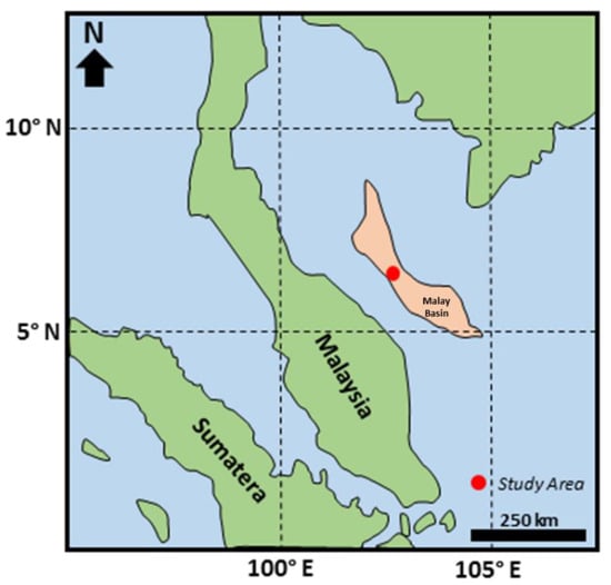
Figure 1.
Geographical map of Peninsular Malaysia. The red circle is the study area location which is located in the Malay Basin.
The main reservoir targets have occurred at D and E formations []. These reservoirs deposited at the fluvial-deltaic system (Figure 2). Group D and E were deposited by progradation stacking of dominantly alluvial/estuarine channels and culminated with localized erosional unconformity []. Group E was occurred in a slightly influenced by a marine at the coastal plain environment, with the sandstone being deposited in delta front and delta plain including distributary mouth bar, shoreface, and channels. Group E has estimated to have 300 m thickness that was deposited by sandstone, siltstone, carbonaceous shale, and coal. Group D, with a range thickness of 300–650 m, comprises siltstone, shale, sandstone, and coal. The most effective source rock in the Northern Malay basin has occurred in groups H and I. Their present-day depth of burial, maturity, and source rock quality related to the effectiveness. The groups of E and D reservoirs are predicted to be charged from the group I source rocks, which reached the gas generation phase by the time the anticlinal traps were generated.
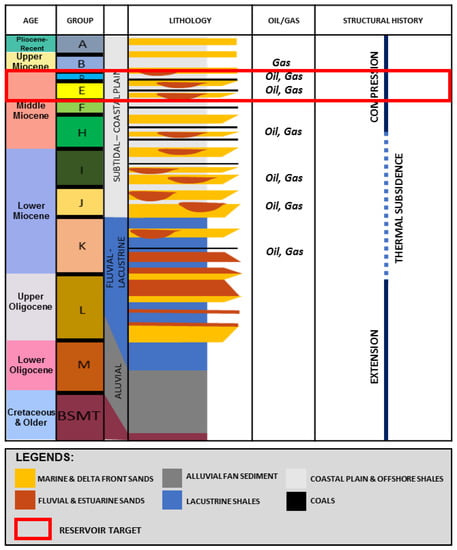
Figure 2.
Regional stratigraphy column of the Malay Basin and the reservoir targets which is highlighted by red rectangular. The reservoir targets are focused on D and E groups (modified from) [].
3. Data Set and Methodology
3.1. Data Set
Facies and hydrocarbon detection were identified by using the integration of well log and seismic data (Figure 3). The dataset used for this research included the wireline logs and seismic data from the northern Malay basin. Post-stack and pre-stack seismic data were used to combine with the well-logs to improve the analysis completion. In this study area, there were eight wells used in this research, i.e., labelled as I-1, I-2. I-3, I-5, I-6, I-7, I-8, and ID-1. Eight well logs were used to do well seismic tie and facies interpretation. Other data from ID-1 and I-8 comprised a core, biostratigraphy, and Formation Micro-Imager (FMI) reports which was used to validate the facies classification.
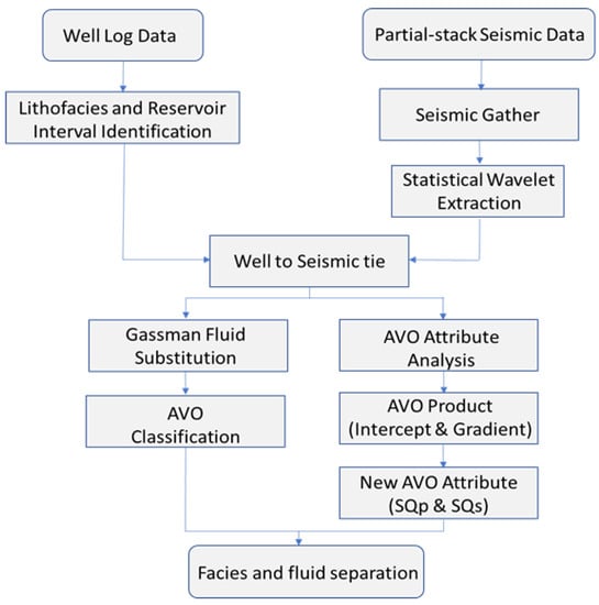
Figure 3.
Amplitude versus offset (AVO) modeling workflow for facies and fluid identification.
Based on 3D seismic data, this field comprised 398,750,000 m2 area. The seismic data included post-stack and pre-stack data (near, mid, and far). The high resolution of structural and stratigraphic features in this research indicated a good quality of seismic data. The polarity of the seismic data was a zero-phase positive peak for increasing acoustic impedance. Furthermore, according to seismic data, the thickness could be captured at about 15 m. The integration of well log and seismic data was essential to increase the confidence in facies interpretation. Nevertheless, well log data showed the vertical changing and the seismic data was qualified to determine facies distribution.
3.2. Methodology
Well log and seismic data had a different domain where well log data had depth domain, and seismic data had time domain. Well seismic tie was needed to convert depth domain to time domain and vice versa. Wavelet and seismic ties were important in forwarding modeling to generate an actual earth model. The match was based on a selection wavelet that created for predicting the model response []. The well-seismic tie depended on measuring the density and sonic logs in generating an acoustic impedance log []. The acoustic impedance combined with the velocity data to derive a reflection coefficient series in time. The seismic data was essential to calibrate to the geology in a well to get a high-quality result of the AVO model.
The first step in a well-seismic tie was calibrating the sonic log, density, and check-shot to create a time-depth relationship (Figure 4). In this project, statistical wavelet extracted from seismic data was the best wavelet for the well convolution. The convolution of reflection coefficient with the corrected wavelet generated synthetic seismograms. The well data that has tied with seismic can be used to interpret the seismic data. The bulk shift, stretch, and squeeze technique were applied in this process to get a higher correlation value. In this study, the range of bulk shift was 0–20 ms. Reducing an uncertainty of geological understanding was obtained following the high-quality correlation between seismic and synthetic seismic data, which created about 70–85% similarity of the extraction of statistic wavelet. The percentages meant the extracted wavelet provided a high correlation. The constant computation windows were between 600 to 1200 ms.
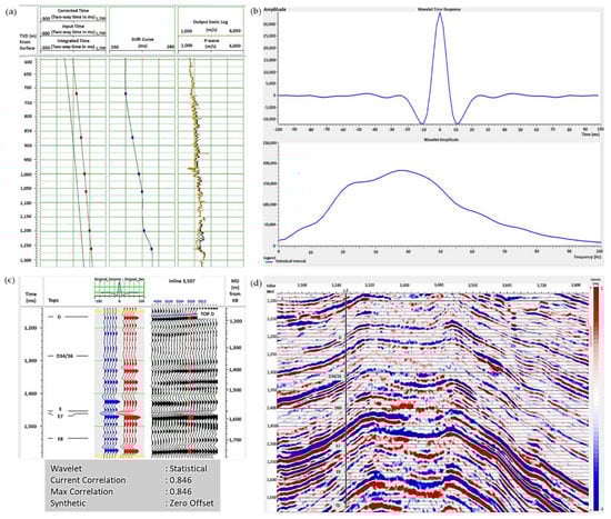
Figure 4.
Well log seismic tie for I-2 log, (a) check shot correction in one of the logs, (b) statistical wavelet with timely response and respective amplitude spectrum on the bottom, (c) an example of a well seismic tie in the research area. The blue seismic traces were the calculated synthetic, and the red seismic traces were the real seismic data using statistical wavelet, and (d) seismic section which was tied with well log.
Facies was a discrete variable that delineated the quality of rock categories and presented the scale of heterogeneities. Facies was characterized by using well log, where different facies showed different petrophysical properties. Petrophysical well log data was interpreted to identify facies which was validated with core reports from some wells. Cut-off from the well log properties were used to characterize well logs facies in research area []. Four different facies classes were defined, i.e., shale, brine sand, gas sand, and coal. The well log responses were integrated with the seismic AVO result to identify facies and hydrocarbon distributions.
The seismic AVO was extensively used in facies prediction and fluid parameter studies []. The AVO attribute was commonly applied to illustrate the relationship between rock physical properties and seismic []. Primary AVO attribute produced the intercept (A) and the reflection-coefficient gradient (B) []. AVO was classified to be four classes based on different amplitude response of gas-sands enclosed by shale. Class I showed the developments include high acoustic impedance sands and the amplitude decrease with offset. Class I had a positive intercept and a negative gradient. Class II produced sands surrounded by shale with small impedance contrast and the amplitude could either increase or decrease with offset. The intercept of class II value was positive or negative, and on the other hand the gradient was negative. Class III for low acoustic impedance sands that were usually gas sand. The amplitude class III increased along with offset and intercept, while the gradients were negatives. Class IV was added to the AVO class, which was mentioned the standard reflection coefficient as negative and decreases while the offset increases. Meanwhile, the intercept of Class IV was negative and the gradient was positive [,,] (Figure 5). Figure 5a showed the character of gas sand on the well log which had high resistivity responses. The amplitude of the gas sands were expected to increase with offset and give negative value for intercept and gradient (Figure 5b,c).
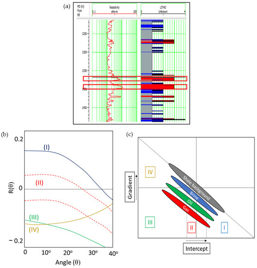
Figure 5.
(a) Characteristic of resistivity log for gas sand reservoir at study area, which was highlighted by red rectangles, (b) AVO response for class 1, 2, 3, and 4, and (c) AVO classes of a seismic reflection based on AVO cross plot.
The geological model or petrophysical analysis in a basin was an essential element in the interpretation of amplitudes. AVO analysis was facilitated by cross plotting AVO intercept (A) and gradient (B). AVO was classified under a variety of reasonable geologic conditions. AVO technique produced a direct hydrocarbon indicator (DHI), lithology separation, and fluid types characterization using angle-stack seismic data based on amplitude contrast in interfaces []. A seismic DHI was characterized as a seismic anomaly pattern that was explained by the presence of hydrocarbons []. A DHI had many characteristics; AVO anomalies, bright spots, and flat spots in general. A DHI interpretation should be suitable with geological interpretation.
Angle seismic-stack was used to create seismic gather as an input of AVO analysis []. Real seismic data, pre-stack seismic data including near, mid, and far, then well log data were integrated to get suitable identification on facies and fluid. The AVO analysis was created by extracting intercept (A) and gradient (B) to be applied as Scaled Poisson’s Ratio change and the new AVO attributes (SQp, and SQs), which created cross plots to classify reservoir fluids and lithological units []. The seismic gather was used as an input for AVO common attributes, including intercept (A) and gradient (B), which was applied by two-terms of Aki-Richards (Figure 6). The common method in gas identification was Scaled Poisson’s Ratio attribute []. Scaled Poisson’s Ratio AVO attribute identification was based on the reservoir fluid content. To enhance the higher quality of separation for hydrocarbon detection and facies separation, the latest methods, SQp and SQs, were also applied. New AVO attributes methods, SQp and SQs, were applied in each interest interval area, to provide a better understanding of facies distribution and hydrocarbon identification.
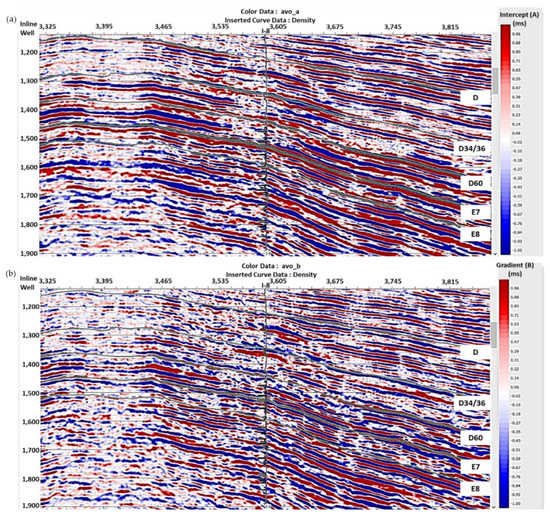
Figure 6.
Xline 5078 intersection for (a) Intercept, (b) gradient.
SQp and SQs methods in well log scale have been successfully patented which was derived from elastic properties parameters []. In the well log scale, SQp attribute response was equivalent to the gamma-ray log and SQs attribute resembled the resistivity for facies and hydrocarbon identification []. SQp and SQs also could be applied in pre-stack stack seismic inversion. In this research, the SQp and SQs were intended to be directly applicable on a seismic scale as new AVO attributes. These methods were proposed to get better separation in facies and hydrocarbon prediction. The study has started with the concept of AVO attributes to understand the SQp and SQs in AVO domain. In AVO method, the potential hydrocarbon reservoirs were defined as an AVO anomaly. The parameters compressional velocity, shear velocity, and density were highly corelated with the anomaly of hydrocarbon and lithologies detection. These correlations defined relationships between the angular reflection coefficients A and B []. As the products of intercept (A) and gradient (B), SQp and SQs have been derived to get more sensitive AVO attributes from the equations:
4. Results and Discussion
Reservoir targets were located at D and E formations. Five horizons were generated based on hydrocarbon intervals; Top D, D34/36, D60, E, and E7. Figure 7 showed the structural model in the top D34/36. The D34/36 time structure base map showed N-E oriented anticline structure and two directions of the fault, i.e., N-S trending faults and E-W trending faults.
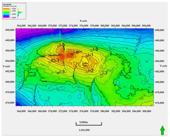
Figure 7.
D34/36 formation of time structure base map of the study area. The base map shows the surface seismic and well locations.
Figure 8 illustrated the seismic amplitude anomalies in D34/36 formation, which was penetrated by the I-8 well location. The seismic section was interpreted as a bright spot of gas accumulation and shown as the strong blue color in that area. These anomalies have been validated with well log interpretation, which established that the interval had high resistivity, low acoustic impedance, and identified as gas sands intervals. AVO attributes have been developed to validate seismic amplitude anomalies to be correlated with gas sands. The seismic was illustrated as a zero phase, with a trough for decreasing acoustic impedance or a peak for increasing acoustic impedance.
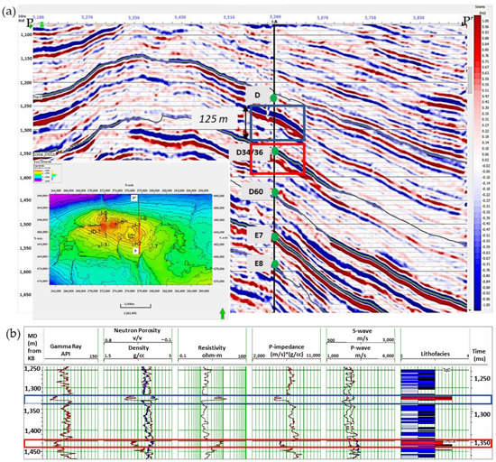
Figure 8.
Seismic and well log comparison for interval D + 49, which was shown in blue rectangles, and D34/36, which was shown in red rectangles (a) Seismic cross section which was penetrated by well log I-8, (b) well log tracts from left to right gamma-ray, neutron and density, resistivity, acoustic impedance, s-wave and p-wave, and facies.
4.1. Facies Identification
Facies was characterized by using well log data, including core and well log report. Facies in well logs were distributed based on petrophysical logs cut-off. The input data in facies identification were the volume of shale, the volume of coal, porosity, and water saturation (Sw). Based on the interpretation, facies were characterized as the gas sand, brine sand, shale, and coal that had different cut-off. Gas sand had less than 0.4 volume of shale, less than one of the volumes of coal, less than 0.7 of effective water saturation, and more than 0.05 effective porosity proposition. Brine sand had less than 0.4 of the volume of shale, less than one of the volumes of coal, and more than 0.7 effective water saturation proposition. Shale had more than 0.4 volume of shale proposition; meanwhile, coal had less than 0.4 volume of clay and more than one volume of coal proposition.
Figure 9 illustrates the facies proportion in wells where facies characteristic in this research area was dominated by shale interbedding with sand. Different color codes were assigned to interpret facies to provide better representation in defining the lithologies. Red was for gas sand, blue was for brine sand, grey was for shale, and black corresponded to coal. The predicted facies was validated by core reports to ensure the result was reliable. The comparison showed a great similarity between the predicted log from petrophysical logs cut-off and measured data from the core reports. The facies logs were later used to validate seismic responses.
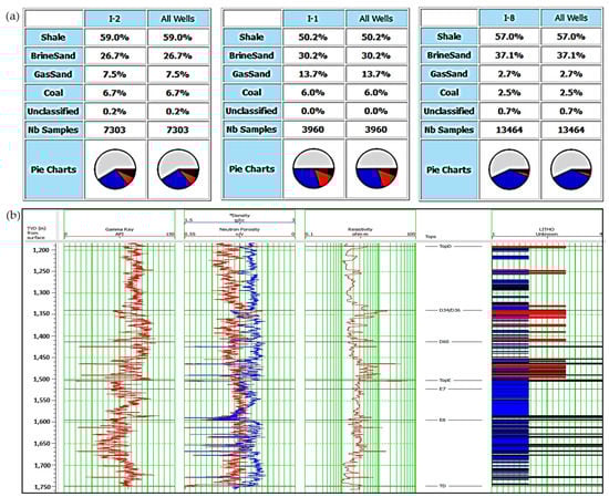
Figure 9.
(a) Facies percentage in I-1, 1-2, and I-8 logs, (b) facies discrimination compared to any logs such as gamma-ray, density, neutron, and resistivity.
4.2. AVO Analysis
The AVO analysis was analyzed to confirm the hydrocarbon presence in the research area. Gassmann’s fluid substitution modeling was generated in the well logs and AVO synthetics for in situ, pure brine, and pure gas cases. Based on Figure 10, the gas-sand had the lowest acoustic impedance followed by pure brine sand. The AVO synthetics from each synthetic showed different responses. AVO synthetics of top in situ and pure gas sand showed the strongest trough compare to AVO synthetics of top pure brine.
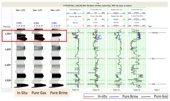
Figure 10.
Gassmann’s fluid substitution in one of the reservoir intervals (Top D34/36) from Well I-8. The red rectangle was the interval of hydrocarbon.
The AVO responses of the in situ synthetic seismic should be the same, according to the AVO response from the original seismic to validate the other analysis scheme. Based on the results, the AVO response of the original seismic was similar to the AVO response of in situ synthetic. The top gas sand was classified into AVO class three, where the amplitude decreased along with the increases of angle and had both negative intercept and gradient. Based on the AVO classification, the gas sand has interpreted as the low impedance sand. Moreover, The AVO response of the pure brine sand was classified into class four, where the amplitude increased with increasing angle and had negative with a positive gradient (Figure 11).
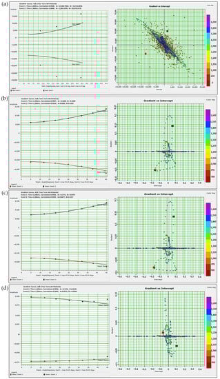
Figure 11.
AVO analysis from some models, (a) original seismic, (b) in situ, (c) pure gas, and (d) pure brine.
The AVO attributes were generated to distinguish between the change in lithology and fluid content by the anomalies identified from AVO analysis. Figure 6 illustrated the AVO responses derived from the product of the intercept and gradient. By combining AVO anomaly and data logs such as density and resistivity, a compatibility between AVO response and the gas sand could be found. AVO attributes, such as Scales Poisson’s Ratio change, SQp and SQs were generated to compare which the most sensitive attributes in detecting the reservoir sand.
Figure 11 showed the application of some AVO attributes for D34/36 interval which was integrated with well log data. As the product of intercept (A) and gradient (B), Scaled Poisson’s Ratio attribute was applied, which showed the negative values at the top of the reservoir and positive response at the reservoir base. Well log responses were integrated to seismic responses to reduce the uncertainties. The I-8 log showed that top D34/36 was gas sand and compared to seismic on D34/36 interval, which was penetrated by well I-8 showed the negative value or orange color. That value was indicated as the hydrocarbon accumulation. The I-3 well logs figured that top D34/36 as the gas sand with low gamma-ray, on the other hand, according to the seismic scale, the hydrocarbon potential was not figured. Comprised of the new attributes, SQp and SQs have been applied to give better separation in differentiate between facies and hydrocarbon separations. These attributes provided a better resolution compared to the Scaled Poisson’s Ratio attribute (Figure 12). By using SQp and SQs attributes, the seismic attribute at I-3 well log position could be captured as hydrocarbon potential, which was shown as a strong negative value or orange color.
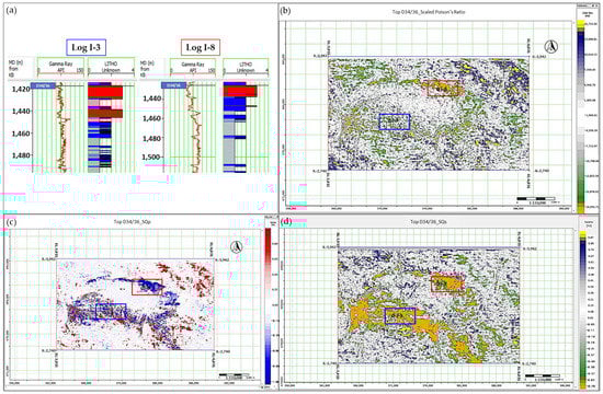
Figure 12.
The methods comparison between Scaled Poisson’s Ratio, SQp, and SQs attributes, (a) Well log I-3 and I-8 showed that top D34/36 was a gas sand interval, (b) Scaled Poisson’s Ratio attribute slice could not capture a gas sand interval in well I-3, (c) SQp attribute slice gave better resolution, which could capture sand area at well I-3. The sand interval was figured as blue color, and (d) SQs attribute gave better resolution which could capture a gas sand area at well I-3. The gas sand interval was figured as orange color.
Figure 13 showed the application of SQp AVO attribute in differentiating the facies. Scaled color from −1 to 1 was considered as the best range to identify the facies. SQp attribute from the seismic scale was compared to log responses e.g., density and resistivity. Both data gave consistency results. In the well log scale, top D, D+49, and D34/36 on I-8 well log location captured the low-density values and had been interpreted as sand intervals. Moreover, the top D, top D + 49, and top D34/36 intervals on the seismic section which was penetrated by I-8 well area showed as a blue color or negative values, which was interpreted as a sand area. It showed a decrease value in SQp attribute at the top of the sand and an increase at the base. Based on the application of the new attribute on the seismic scale, SQp AVO attribute provided high sensitivity in differentiating the facies.
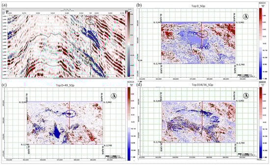
Figure 13.
Application of SQp attribute to distinguish facies. (a) Seismic section which was penetrated by I-8 well log showed that the sand area was interpreted as a blue color. The red circle was top D, the blue circle was the top D+49, and the green circle was the top D34/36. These circles illustrated the consistency result between SQp attribute application and density characteristic for facies prediction, (b) SQp attribute slice for Top D zone. The red circle was the sand area for D interval, which was penetrated by I-8 log, (c) seismic attribute slice for top D+49 ms zone. The blue circle was the sand area for D+49 interval, which was penetrated by I-8 log, and (d) seismic attribute for top D34/36 zone. The green circle was the sand area for D34/36 interval, which was penetrated by I-8 log.
Another latest applied AVO attribute was SQs attribute. Figure 14 showed the application of SQs AVO attribute in differentiating hydrocarbon composition. SQs attribute from the seismic scale was compared to log responses e.g., hydrocarbon saturation. Based on the seismic section, top D+49 and top D34/36 intervals, which were penetrated by I-8 well were classified as the gas sand reservoir. The top gas sands were identified as the AVO class three. The gas accumulation showed an orange color or negative value. The extraction of this attribute generated the best way to show AVO anomaly, and its values was ranging from−0.8 to 0.9. Moreover, it was integrated with the log responses, which showed that both intervals were identified as gas sand intervals. In the log scale, these two intervals gave the high hydrocarbon saturation values. Based on the application of the new AVO attribute, SQs attribute provided the best indicator of fluid separation.
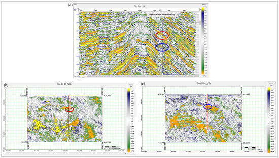
Figure 14.
Application of scale of quality factor of S-wave (SQs) attribute to distinguish fluid distribution. (a) Seismic intersection which was penetrated by I-8 well log showed that the gas zone identified as an orange color. The red circle was top D + 49 while the blue circle was top D34/36. These circles illustrated the consistency result between SQs attribute application and hydrocarbon saturation log responses for the hydrocarbon prediction, (b) seismic attribute slice for Top D + 49 ms zone. The red circle was the gas sand area for top D + 49, which was penetrated by I-8 log, and (c) seismic attribute slice for the top D34/36 zone. The blue circle was the gas sand area for top D34/36, which was penetrated by the I-8 log.
5. Conclusions
According to the several seismic intervals in this research, the identified gas accumulation is shown by bright spot anomalies. One advanced method is by correlating seismic amplitude anomalies with AVO analysis. The AVO result shows that the gas in the target area is classified as AVO class three. It shows a decrease in amplitude and an increasing angle, moreover, it has a negative intercept and gradient. SQp and SQs are proposed as new AVO attributes to distinguish facies and fluid, furthermore, it is successfully generated. These attributes compare to Scaled Poisson’s Ratio attribute. Through numerical simulation and application in a field northern Malay basin, SQp and SQs demonstrates a better performance than Scaled Poisson’s Ratio attribute in facies and hydrocarbon prediction. By comparing new attributes to Scaled Poisson’s Ratio, the new attributes are less ambiguous in facies and hydrocarbon prediction. The proposed attributes can predict facies and the presence of possible hydrocarbon sand effectively, which can reduce exploration risk. As the new attributes, SQp and SQs values are validated with logs data; therefore, it shows the regularity of the changing. The well log shows that the gas sand areas have high resistivity and low acoustic impedance. The SQp AVO attribute provides the best separation of facies, while the SQs AVO attribute is a suitable indicator for fluid identification. The proposed AVO attributes methods are suitable to be used as other options in facies and fluid determinations. Moreover, the new technique is potentially examined in any field and to extend the application in other cases, e.g., the carbonate reservoir.
Author Contributions
Conceptualization, T.K.R.; methodology, T.K.R. and M.H.; software, T.K.R.; validation, T.K.R., M.H., L.A.L., and Z.A.R.; formal analysis, T.K.R.; investigation, T.K.R., M.H., L.A.L., and Z.A.R.; resources, T.K.R. and M.H.; data curation, T.K.R.; writing—original draft preparation, T.K.R.; writing—review and editing, T.K.R., M.H., L.A.L., and Z.A.R.; visualization, T.K.R. and L.A.L.; supervision, M.H. and L.A.L. All authors have read and agreed to the published version of the manuscript.
Funding
This research was funded by UTP fundamental research grant with grant number 015LCO-224.
Acknowledgments
The authors would like to thank PETRONAS Malaysia for providing the data for this study. We would like to express our appreciation to Centre of Seismic Imaging and Geoscience department Universiti Teknologi PETRONAS colleagues for supporting us throughout the project. Huge gratitude to UTP fundamental research grant with cost centre 015LCO-224 for granting this research. We acknowledge to CGG Company for providing Hampson Russell software licensing, Schlumberger Company for providing Petrel software licensing, and Ikon Science for providing Rokdoc software licensing.
Conflicts of Interest
The authors declare no conflict of interest.
References
- Al-Baldawi, B.A. Reservoir Characterization and Identification of Formation Lithology from Well Log Data of Nahr Umr Formation in Luhais Oil Field, Southern Iraq. J. Sci. 2016, 57, 436–445. [Google Scholar]
- Kamilah, T.; Azzahra, Y.F.; Setiadi, W.P.; Jasmine, M. Artificial Intelligence Methods Usage in Analysing Lithofacies and Pore Pressure, Bintuni Basin, West Papua, Indonesia. In Proceedings of the Joint Convention Malang, East Java, Indonesia, 25–28 September 2017. [Google Scholar]
- Han, D.; Batzle, M.L. Gassmann’s equation and fluid-saturation effects on seismic velocities. Geophysics 2004, 69, 398–405. [Google Scholar] [CrossRef]
- Rutherford, S.R.; Williams, R.H. Amplitude-versus-offset variations in gas sands. Geophysics 1989, 54, 680–688. [Google Scholar] [CrossRef]
- Hussein, M.; Abu El-Ata, A.; El-Behiry, M. AVO analysis aids in differentiation between false and true amplitude responses: A case study of El Mansoura field, onshore Nile Delta, Egypt. J. Pet. Explor. Prod. Technol. 2019, 10, 969–989. [Google Scholar] [CrossRef]
- Carney, S.; Aziz, I.A.; Martins, W.; Low, A.; Kennedy, J. Reservoir Characterisation of the Mio-Pliocene Reservoirs of PM301 in the North Malay Basin. In Proceedings of the CPS/SPE International Oil & Gas Conference and Exhibition in China, Beijing, China, 8–10 June 2010; pp. 1–25. [Google Scholar] [CrossRef]
- Ghosh, D.; Halim, M.F.A.; Brewer, M.; Viratno, B.; Darman, N. Geophysical issues and challenges in Malay and adjacent basins from E&P perspective. Lead. Edge 2010, 29, 436–449. [Google Scholar]
- Nieto, J.; Batlai, B.; Delbecq, F. Seismic lithology prediction: A Montney shale gas case study. CSEG Rec. 2013, 38, 34–43. [Google Scholar]
- Hermana, M.; Ngui, J.Q.; Sum, C.W.; Ghosh, D.P. Feasibility Study of SQp and SQs Attributes Application for Facies Classification. Geosciences 2018, 8, 10. [Google Scholar] [CrossRef]
- Hermana, M.; Ghosh, D.P.; Sum, C.W. Optimizing the Lithology and Pore Fluid Separation Using Attenuation Attributes. In Proceedings of the Offshore Technology Conference Asia, Kuala Lumpur, Malaysia, 22–25 March 2016; Volume 2016, pp. 3196–3203. [Google Scholar] [CrossRef]
- Hermana, M.; Lubis, L.; Ghosh, D.P.; Sum, C.W. New Rock Physics Template for Better Hydrocarbon Prediction. In Proceedings of the Offshore Technology Conference Asia Kuala, Lumpur, Malaysia, 22–25 March 2016; Volume 2016, pp. 2900–2905. [Google Scholar] [CrossRef]
- Lew, C.L.; Hermana, M.; Ghosh, D.P. Improvised approach using SQp-SQs attributes for hydrocarbon prediction: A field case study in Malay Basin. SEG Tech. Program Expand. Abstr. 2018, 2018, 3105–3109. [Google Scholar] [CrossRef]
- Mansor, M.Y.; Rahman, A.H.A.; Menier, D.; Pubellier, M. Structural evolution of Malay Basin, its link to Sunda Block tectonics. Mar. Pet. Geol. 2014, 58, 736–748. [Google Scholar] [CrossRef]
- Madon, M.; Yang, J.-S.; Abolins, P.; Abu Hassan, R.; Yakzan, A.M.; Zainal, S.B. Petroleum systems of the Northern Malay Basin. Bull. Geol. Soc. Malays. 2006, 49, 125–134. [Google Scholar] [CrossRef]
- Madon, M.B.H. Tectonic Evolution of the Malay and Penyu Basins, Offshore Peninsular Malaysia. Ph.D. Thesis, Unversity of Oxford, Oxford, UK, February 1995. [Google Scholar]
- Madon, M.B.H.; Abolins, P.; Hoesni, M.J.B.; Ahmad, M.B. Malay Basin. In The Petroleum Geology and Resources of Malaysia; Selley, R., Meng, L.K., Eds.; Petronas: Kuala Lumpur, Malaysia, 1999; pp. 173–217. [Google Scholar]
- El Kadi, H.H.; Shebl, S.; Ghorab, M.; Azab, A.; Salama, M. Evaluation of Abu Madi Formation in Baltim North & East gas fields, Egypt, using seismic interpretation and well log analysis. NRIAG J. Astron. Geophys. 2020, 9, 449–458. [Google Scholar] [CrossRef]
- Myint, K.; Ko, K.; Lwin, H.M.Y. Lithology prediction and fluid discrimination in Block A6 offshore Myanmar. In Proceedings of the 10th Biennial International Conference & Exposition, Le Meridien, Kochi, India, 23–25 November 2013; p. 141. [Google Scholar]
- Li, Y.; Downton, J.; Xu, Y. Practical aspects of AVO modeling. Lead. Edge 2007, 26, 295–311. [Google Scholar] [CrossRef]
- Ismail, A.; Ewida, H.F.; Al-Ibiary, M.G.; Zollo, A. Application of AVO attributes for gas channels identification, West offshore Nile Delta, Egypt. Pet. Res. 2020, 5, 112–123. [Google Scholar] [CrossRef]
- Foster, D.J.; Keys, R.G.; Lane, F.D. Interpretation of AVO anomalies. Geophysics 2010, 75, 75A3–75A13. [Google Scholar] [CrossRef]
- Break, F.; Veeken, P.; Rauch-davies, M. AVO attribute analysis and seismic reservoir characterization. First Break 2006, 24, 41–52. [Google Scholar]
- Castagna, J.P.; Swan, H.W. Principles of AVO crossplotting. Lead. Edge 1997, 16, 337–344. [Google Scholar] [CrossRef]
- Nixon, S.; Hallam, T.; Constantine, A. Ranking DHI attributes for effective prospect risk assessment applied to the Otway Basin, Australia. In Proceedings of the Australian Exploration Geoscience Conference, Sydney, Australia, 18–21 February 2018. [Google Scholar]
- Kim, Y.-J.; Cheong, S.; Chun, J.-H.; Cukur, D.; Kim, S.-P.; Kim, J.-K.; Kim, B.-Y. Identification of shallow gas by seismic data and AVO processing: Example from the southwestern continental shelf of the Ulleung Basin, East Sea, Korea. Mar. Pet. Geol. 2020, 117, 104346. [Google Scholar] [CrossRef]
- Castagna, J.P.; Swan, H.W.; Foster, D.J. Framework for AVO gradient and intercept interpretation. Geophysics 1998, 63, 948–956. [Google Scholar] [CrossRef]
Publisher’s Note: MDPI stays neutral with regard to jurisdictional claims in published maps and institutional affiliations. |
© 2020 by the authors. Licensee MDPI, Basel, Switzerland. This article is an open access article distributed under the terms and conditions of the Creative Commons Attribution (CC BY) license (http://creativecommons.org/licenses/by/4.0/).