Virtual UV Fluorescence Microscopy from Hematoxylin and Eosin Staining of Liver Images Using Deep Learning Convolutional Neural Network

Featured Application

The proposed solution allows for the digital conversion of the image of a hematoxylin–eosin-stained slide, using a convolutional neural network, to an image resembling a fluorescent image obtained with a UV microscope.

Abstract

The use of UV (ultraviolet fluorescence) light in microscopy allows improving the quality of images and observation of structures that are not visible in visible spectrum. The disadvantage of this method is the degradation of microstructures in the slide due to exposure to UV light. The article examines the possibility of using a convolutional neural network to perform this type of conversion without damaging the slides. Using eosin hematoxylin stained slides, a database of image pairs was created for visible light (halogen lamp) and UV light. This database was used to train a multi–layer unidirectional convolutional neural network. The results of the study were subjectively and objectively assessed using the SSIM (Structural Similarity Index Measure) and SSIM (structure only) image quality measures. The results show that it is possible to perform this type of conversion (the studies used liver slides for 100× magnification), and in some cases there was an additional improvement in image quality.

1. Introduction

Classical optical microscopy is one of the foundations of medical and biological research [1,2]. The classic solution is based on the human eye and many methods have been used to improve the image quality in order to highlight the desired features. Various physical methods are used, such as microstructure illumination methods, work with the handling of filters, including the use of multispectral and hyperspectral methods, as well as biochemical methods, where image segmentation is performed using dedicated staining [3].

An extremely important element in the development of microscopy, although often overlooked, is the change in the method of image analysis. The introduction of computer image analysis methods combined with knowledge-based methods, in particular machine learning methods [4], allows one to extend the possibilities of microstructure analysis. Improving image quality or extracting essential features is not only essential for systems that perform automatic analysis, but also for human specialists using CADx (computer aided diagnosis) systems [5,6]. This possibly essential part of the important information in a digital image is available but is not visible to the human eye, or its microstructure is too complex for the human brain, even a trained specialist, to analyze.

A typical solution used in classical microscopy is the use of dedicated staining and a bright field microscope [7]. In this configuration, an ordinary lamp (halogen or LED) is the light source that passes through the slide, and then, when magnified by an optical system, is visible to the eye or the camera sensor. This solution is cheap and does not quickly degrade the microstructure in the slide.

The development of the image acquisition technique has led to the expansion of microstructure acquisition methods not only in the visible light spectrum. One of the known methods of image acquisition is fluorescence microscopy [8,9]. This method uses a lamp with a UV light which excites the sample when it hits the sample. As a result of this excitation, light is emitted of a different wavelength, which is observed by the optical system of the microscope. This technique can be used when the observer is a human if the wavelength is within the sensitivity of the human eye. The use of a digital camera enables the analysis of wavelengths outside the sensitivity range of the human eye’s light spectrum.

The most important disadvantages of fluorescence microscopy [7] are photobleaching and photo damage of observed tissue [10,11,12]. These processes are not fully understood and manifest themselves by burning off the observed material. This means that a longer observation of the same section of a slide results in a gradual irreversible destruction of the microstructures. It depends on the wavelength—the shorter the wavelength, the faster the process is. This is especially troublesome in research where the same structures are often required for analyses. The use of digital microscopy with the use of a slide scanner reduces this problem because the acquisition is done once and the analysis is performed on the computer screen. Unfortunately, both fluorescent microscopes and fluorescent slide scanners are much more expensive than typical microscopes. An exemplary reason is the cost of dedicated lenses.

1.1. Contribution of the Paper and Related Works

The paper proposes a solution for digital conversion of the image of a slide stained with H&E (hematoxylin and eosin) [13] to a form resembling an image obtained with the use of fluorescence. The main contributions of the paper are:

• Possibility to use a digital bright field microscope in place of a fluorescence microscope,
• Limiting the influence of photobleaching and photo damage in the slide microstructure,
• Analysis of the possibility of using deep learning convolutional neural networks to implement this type of conversion.

As the research material, slides with sections of human livers were used. The confirmation of the possibility of performing this type of image conversion gives us a chance to use a similar method to convert images of other biological structures.

The work is inspired by other research in the field of microscopic image conversion. One of the active areas of research is the digital staining of slide images [14,15,16,17,18]. As the staining process is a biochemical process, it requires proper preparation of a section, the use of chemical reagents (often expensive or hazardous to health), and time and human resources. The use of deep learning neural networks is an interesting alternative to classical biochemical staining.

Another area of inspiration for research is improving image quality. The microscopic images often have poor contrast and sharpness. This is due to many factors such as the quality of biological material, the quality of the staining process, and the quality of the image acquisition system (cameras and lenses). A serious problem is the influence of thickness and thickness variation of biological material during the cutting. The use of computer methods allows one to improve the visual quality of the image. Additionally, it is possible to use super resolution methods to increase image resolution [19,20,21,22].

1.2. Content of the Paper

Section 2 describes the microscopic images of the liver sections. The same section introduces the virtual imaging solution and describes the individual blocks of the solution. Section 3 presents the results of the image processing, in particular the results for the applied image quality assessment metrics. The discussion takes place in Section 4. Final conclusions and future work are described in Section 5.

2. Materials and Methods

The proposed and tested solution uses a convolutional neural network [23,24,25] that transforms the recorded color images (RGB) into a virtual fluorescence UV image. In the learning and testing phases, the solution presented in Figure 1 is used. During normal operation, the solution presented in Figure 2 is used. Individual blocks are described in the following subsections.

2.1. Liver Microscopic Images

The material consisted of 52 slides showing cases of liver steatosis obtained from autopsy cases. There are various causes of fatty liver disease, including the use of ethyl alcohol, that can manifest as liver steatosis, steatohepatitis, and cirrhosis. It is well known that excessive ethanol consumption is a major public health problem and causes over 60% of chronic liver disease in some countries [26]. It should be noted that short-term consumption of 80 g of ethanol per day usually causes mild, reversible heaptic changes, including fatty liver. Chronic exposure to 40–80 g of alcohol per day can cause serious injury [26].

Steatosis is also a manifestation of non-alcoholic fatty liver disease (NAFLD), that can mimic the spectrum of changes seen in fatty liver in alcoholics. NAFLD is often associated with metabolic syndrome [26].

Hepatocellular steatosis begins with the accumulation of fat in the centrilobular hepatocytes (the epithelial cells of the liver). Usually, steatosis is observed as microvesicular: lipid droplets are small and macrovesicular: lipid droplets are large [26].

Both types of steatosis are very often observed in one slide. As a result, the hepatocyte takes the shape of a ring with the nucleus displaced to the peripheral part of the hepatocytes, that mimics the fatty tisue cells, adipocytes [27]. There are various causes of steasosis, not just alcohol consumption, including agents like amiodarone and methotrexate. Drug/toxin associated liver injury with steatosis manifests itself microscopically mailny as hepatocellular microvesicular steatosis of the liver, often associated with acute liver disfunction [26].

An exemplary pair of acquired images of steasosis is shown in Figure 3. Visible hepatocytes with lipid droplets that have been dissolved during the tissue process (dehydration in a series of alcohols) and hepatocytes with a signet ring with a large droplet of lipids in the cytoplasm are visible as white rounded spots in the color of H&E (black in the UV fluorescence) [27] with a compressed nucleus in the peripheral part of the hepatocytes.

There are also hepatocytes without steatosis, that are large polyhedral cells. Regular hepatocytes have at least six surfaces. The H&E staining cytoplasm is eosinophilic. The nuclei of hepatocytes are large, spherical, cells with two or more nuclei also observed, some of them polyploid. The tubular space between two hepatocytes is defined as bile canaliculus, and the hepatocytes are also in contact with the wall of sinusoid through perisunosidal space of Disse [28].

2.2. Data and Acquisition System

The study used its own database of liver samples, which were described by a patomorphologist. The database contains 52 slides stained with H&E. The microscope Imager D1 (Carl Zeiss) and the Axio–CamMRc5 camera with $2584\times 1936$ resolution in the visible range were used for image acquisition with FS 43 filter set for fluorescence. The images were recorded in pairs, i.e. for a specific position of the slide in relation to the lens, an RGB image (work in bright mode) and a UV image (work in fluorescent mode) were recorded successively using 100× magnification (10× objective). Images were recorded with the AxioVision (Zeiss) software in the uncompressed ZVI format and saved in the 16–bit mode. Since the camera used is color, with a Bayer matrix filter, some mosaic artifacts related to the demosaicing algorithm are observed [29]. The acquisition was done for the same camera settings (in particular the exposure time). Images were converted to 16-bit TIFF per channel using the Bio-Formats library/tools (’bfconvert’ command) [30].

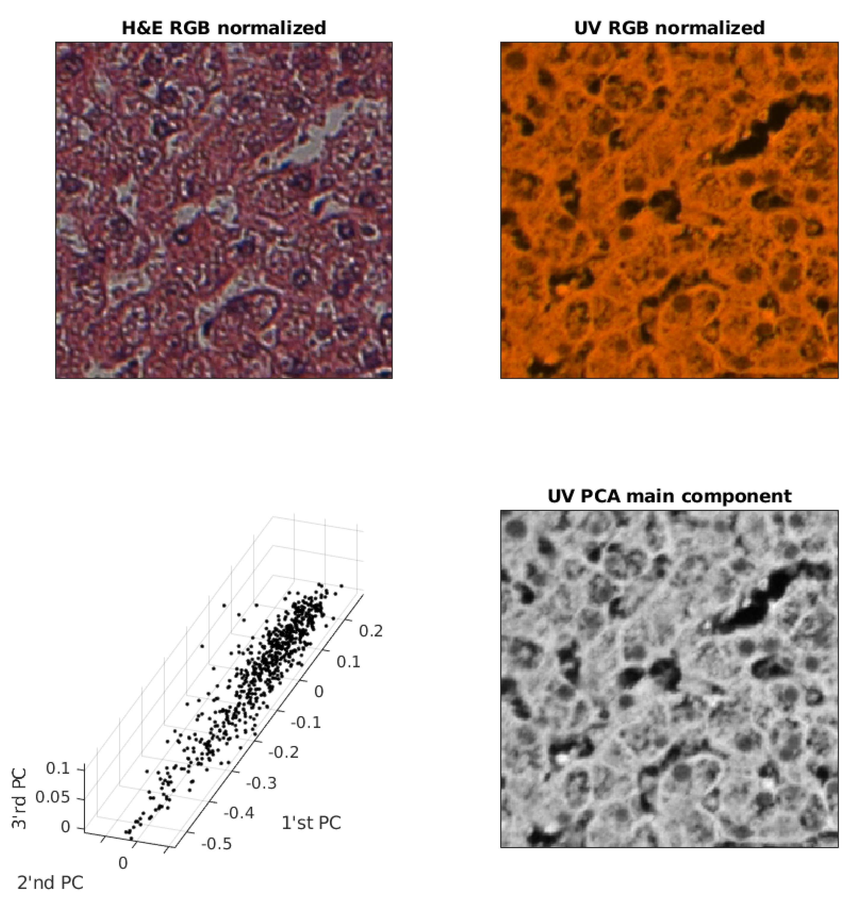
2.3. UV (RGB) Image Redundancy

Since the camera is a color RGB camera, the UV image may contain redundant information. The UV image is the result of the interaction of monochromatic light with biological structures. It is usually close to monochromatic light, that allows the use of a more optimal color space than RGB. In order to verify whether the UV (RGB) image can be converted to a UV image in shades of gray, the PCA algorithm [31] (Principal Component Analysis) was used. The PCA algorithm enables the estimation of a new non-redundant color space for the input RGB image [32,33,34]. This is important for the training algorithm, because if the output image can be a grayscale image, the number of parameters (weights) to be trained will be smaller. RGB color image requires three times more weights in the last layer and reducing the number of parameters is important for the speed of convergence and the reduction of false color generation.

An example of removing redundancy from a UV RGB image is shown in Figure 4. In order to improve the image quality of the first three main components, a random sample for 1% of the pixels is shown.

2.4. Spatial Alignment of Pairs of Images

Care was taken not to shift the stage with the slide during switching the optical system between the halogen and UV lighting modes. However, even slight mechanical vibrations can do so, which is critical to the learning process. For this reason, the images have been automatically aligned. The maximum shift observed was 25 pixels, which is unacceptable for a legitimate conversion.

Image alignment was limited to X–Y translation (image rotation was not necessary), which allowed for a good convergence of the alignment process. Before image alignment, it became necessary to adjust the image characteristics. Due to the differences between the way the slide is illuminated (from the top for the UV lamp and from the bottom for the bright field for the halogen lamp), it was necessary to invert one of the images. Only one H&E RGB image channel-blue was used. Automatic image alignment was done using the ‘imregcorr’ function [35] from Matlab.

2.5. Contrast Normalization

Contrast normalization using z–score has been used as part of image preprocessing to normalize images [36]. Slides can vary in thickness, which affects the amount of light that is transmitted or reflected.

Normalization using the minimum and maximum values of the image is not a good choice, as there are often various artifacts in the slides that can strongly distort normalization. For this reason, fit-based normalization to the Gaussian distribution model was used for the histogram. The slide histograms are a Gaussian mixture [37] with two peaks plus asymmetry, but this type of normalization is less sensitive to outliers, that is, problem of min–max normalization. An example of normalization is shown in Figure 5. The following formulas are used for normalization for ’uint8’ data type:

$$Y(x,y)=\frac{255}{6}\left(\frac{X(x,y)-mean\left(X\right)}{std\left(X\right)}+3\right),$$

(1)

where x and y are pixel coordinates, X is the input pixel value, and Y is the output pixel value.

2.6. Deep Learning Convolutional Neural Network (ConvNN)

A unidirectional multi–layer convolutional network was proposed for the image conversion task. It is a heteroassociative type network with four convolutional layers. The task of teaching this type of network is to obtain an approximator (using regression) that reconstructs the UV image in grayscale (as the main PCA component) from the RGB color image. The regression criterion is MSE (mean squared error). The input image and the output trainer are normalized. The network diagram is presented in Figure 6, and the exact configuration of the layers is given in

Table 1. Configuration of layers.

No.	Name	Type	Activations	Learnables
1	imageinput	Image Input	$[256\times 256\times 3]$	-
	$[256\times 256\times 3]$ images
2	conv_1	Convolution	$[252\times 252\times 128]$	Weights $[5\times 5\times 3\times 128]$
	128 $[5\times 5\times 3$] convolutions			Bias $[1\times 1\times 128]$
	with stride [1 1] and padding [0 0 0 0]
3	relu_1	ReLU	$[252\times 252\times 128]$	-
4	conv_2	Convolution	$[248\times 248\times 256]$	Weights $[5\times 5\times 128\times 128]$
	256 $[5\times 5\times 128]$ convolutions			Bias $[1\times 1\times 256]$
	with stride [1 1] and padding [0 0 0 0]
5	relu_2	ReLU	$[248\times 248\times 256]$	-
6	conv_3	Convolution	$[244\times 244\times 256]$	Weights $[5\times 5\times 256\times 128]$
	256 $[5\times 5\times 256]$ convolutions			Bias $[1\times 1\times 256]$
	with stride [1 1] and padding [0 0 0 0]
7	relu_3	ReLU	$[244\times 244\times 256]$	-
8	conv_4	Convolution	$[242\times 242\times 1]$	Weights $[3\times 3\times 256]$
	1 $[3\times 3\times 256]$ convolutions			Bias $[1\times 1]$
	with stride [1 1] and padding [0 0 0 0]
9	regressionoutput	Regression	-	-
	$[242\times 242\times 1]$ MSE	Output

.

The neural network was trained with the following parameters: training algorithm is SGDM (stochastic gradient descent with momentum) [38,39], initial learn rate is 0.05, momentum is 0.9, gradient threshold is 0.05, mini batch size is 50 and maximal number of epochs is 50. The mini batch size was optimized for maximum use of GPU memory.

Matlab R2020a was used for learning with some modifications. The input images have a resolution of $1000\times 800$ pixels. Such a large size is problematic due to the amount of available RAM in the GPU and the need to store different images simultaneously. A typical solution is training with lower resolution patches which are selected from random positions from the original images. This network uses patches with a size of $256\times 256$ pixels. One problem is that Matlab’s ‘randomPatchExtractionDatastore’ function creates a pair of patches with the same resolution. This makes it necessary to generate a pixel output at the edges, which is associated with a number of artifacts. For this reason, a custom function was created that creates pairs of sizes $256\times 256\times 3$ and $242\times 242\times 1$ for the network input and output respectively.

A computer with two GPU cards Nvidia GeForce GTX 1080 Ti (11178MB RAM, CUDA 11) and Intel Core i7–8700 CPU 3.20GHz processor with 40GB RAM, Linux Debian 10 was used for learning. The learning time was about 8 h.

2.7. Evaluation of Results

The image conversion method was tested with the use of a second database that uses the original database. The resolution of the original images is high and only a fragment of the image was used in the learning process. Other parts of the original images were used for testing. The learning criterion is MSE, but the use of image quality metrics is better to judge final image conversion. There are many image quality metrics, both objective and perceptual (subjective) [40,41,42].

One of the metrics is the SSIM index [43] (Structural Similarity Index Measure), which contains three internal indicators: the luminance term, the contrast term and the structural term. SSIM enables the weighing of individual components and the results show the overall SSIM (all weights equal to 1) and the SSIM only for the structure component (weights for luminance $\alpha$ and contrast $\beta$ terms equal to 0, weight for the structure $\gamma$ term equal to 1). The following formula is used to calculate the SSIM index:

$$SSIM(A,B)={\left[l(A,B)\right]}^{\alpha }·{\left[c(A,B)\right]}^{\beta }·{\left[s(A,B)\right]}^{\gamma },$$

(2)

where, A and B are reference and tested images, $l(.,.)$ is luminance function, $c(.,.)$ is contrast function and $s(.,.)$ is structure function.

3. Results

The results of the work of the entire system, in particular the neural network, are presented in this section. Two SSIM metrics were used to evaluate the quality of the virtual slides.

3.1. Mechanical Shifts

The estimated shifts for pairs of images are shown in the histogram in Figure 7. Most position errors are a few pixels (Euclidean metric), but sometimes there are outliers. Shift estimation allows the compensation for these acquisition errors.

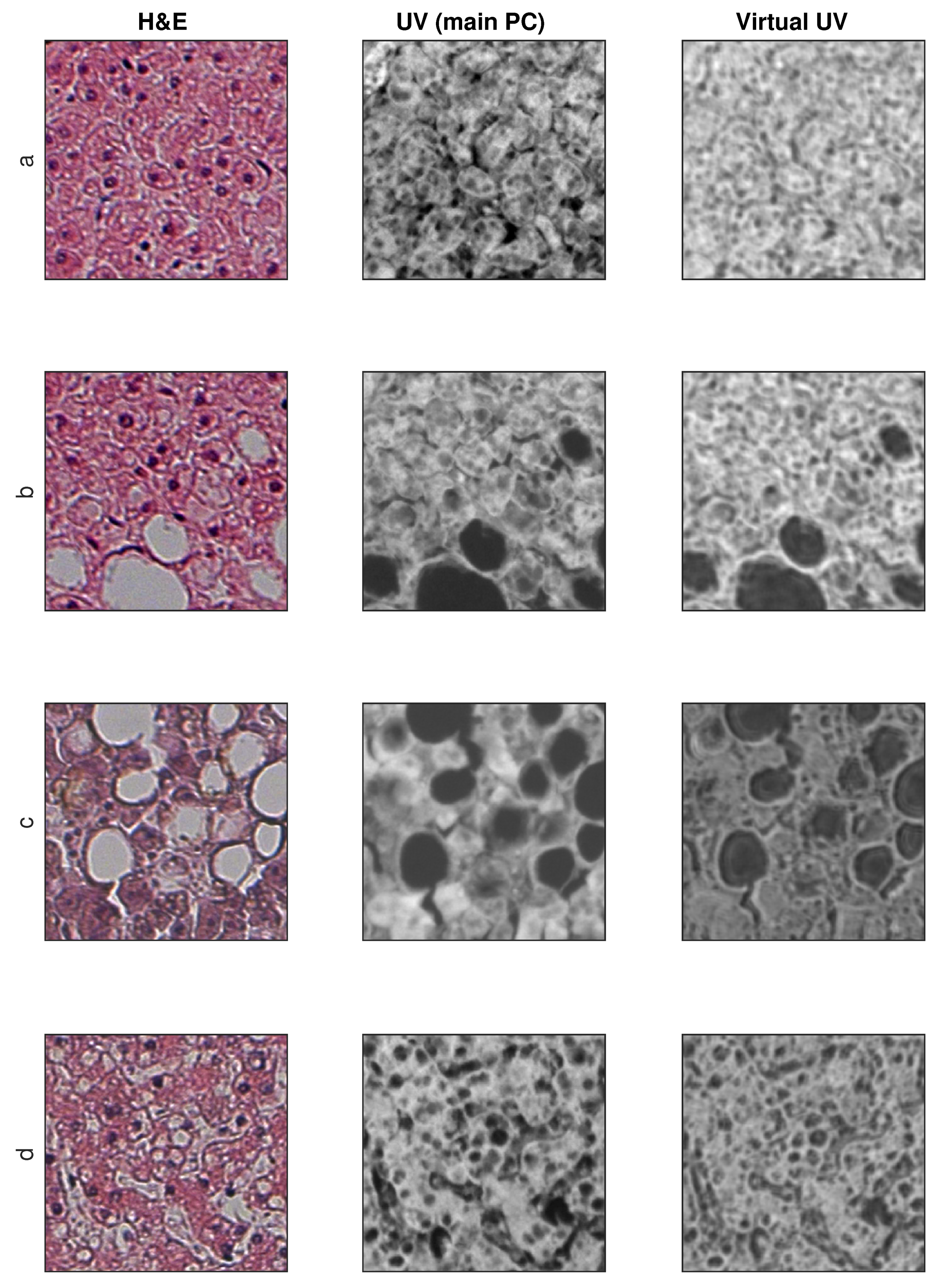
3.2. Exemplary Results

The testing database is derived from the original images database, and these are pairs of images that are not part of the training base and are independent of each other (no overlap).

There are 416 image pairs for network testing. Additionally, the results for the same number of pairs teaching the network are presented. Usually a neural network works better for training images than for testing images. The input H&E image has a resolution of $256\times 256$ and the reference UV and output images have a resolution of $242\times 242$.

Sample training and testing images are shown in Figure 8 and Figure 9, where H&E is RGB input image, UV (main PC) is a preprocessed UV training image and virtual UV is the output image of the convolutional neural network.

3.3. SSIM and SSIM (Structure Only) Metrics

SSIM values range from $〈0-1〉$, with 0 being no similarity and 1 being the perfect match between a pair of pictures. As the database is relatively large, instead of providing values for several images or only the average value for the bases, it was decided to use the Monte Carlo methodology [44,45] to show the histograms of SSIM indexes.

The histograms for the full SSIM metric and the simplified (structure only) are shown in Figure 10.

4. Discussion

4.1. Discussion of Results

The paper shows that the preparation of learning data requires a thorough analysis of the acquisition process. Mechanical problems were identified and an algorithmic solution was proposed for compensation.

The proposed solution confirms the possibility of converting an H&E color image to a UV virtual image. The random results presented in Figure 8 and Figure 9 show a very high similarity between the real UV image (main PC) and that created by the neural network. It should be noted, however, that not all elements of the structure are mapped, for example in Figure 8c, the dark area in the center of the image.

The output images have not undergone additional contrast correction as it may cause changes in image perception (an image with higher contrast is usually considered better). The neural network has the last layer of the regression type, so the mapping comparison should be without the contrast correction of the output image.

The feature of UV images is higher optical resolution in relation to images in the visible light range. This means that the neural network can to some extent perform image enhancement operations in terms of improving resolution.

In the subjective perceptual assessment of images, it seems that the network reproduces smaller than larger structures relatively well. This is visible as the loss of the brightness value of the images for larger uniform structures, for example the light areas in Figure 9c, or the dark areas in Figure 8b–c (sinusoids). Since the lattice is of the convolutional type, individual convolution operations have their range of influence both within one layer and within within all. Increasing the size of convolution nuclei could improve the quality of work, but it would be necessary to increase their number and training time.

The loss of the brightness values for larger areas means that the neural network behaves like a high pass or band pass filter. This does not mean that the low–frequency spatial component is completely removed. Figure 9c shows the differences between the original UV image (main PC) and the reconstruction. The neural network fringes around the edges (lipid droplets regions that have been dissolved during the tissue process, especially). Interestingly, the introduction of this type of artifact improves the visual quality of the image. This is typical of unsharp mask filters [46]. The reconstructed image is visually sharper than the original. This type of operation, although the picture seems to be better for humans, results in deterioration of the SSIM values. For this reason, an attempt to unambiguously assess the quality with the use of SSIM is not fully adequate. The use of general blind measures is also not correct because histological images have their own specificity. Since the neural network can correct images, measure values should be treated with caution.

The study proposes the use of two quality assessment indicators: SSIM and SSIM (structure only). Both indicators were used to evaluate the results for both the training and testing images. The mean values of SSIM and SSIM (structure only) are close to $0.6$ and $0.5$, respectively. In the case of pairs of training images, they are obviously larger because the neural network is trained by them and there is some matching. As the neural network has problems with mapping the brightness of larger areas, it was decided to use the simplified SSIM only for the structure. The values for SSIM (structure only) are shifted on average by about $+0.1$. This means that the neural network reproduces the structure relatively well. Achieving high SSIM values around 0.9–1.0 is in practice unlikely because one of the components of the original H&E and UV (RGB) images is noise and tissue granulation. Noise is acquired and can be reduced by longer exposure. Granulation is a feature of biological material because it contains many small structures. In the process of image acquisition, depending on the lighting (visible/UV light), optical effects of invisible objects may be visible directly due to diffraction and interference. For these reasons, it is unlikely that a network with a very high SSIM will be obtained.

4.2. Discussion Related to Other Works

Image conversion task is an active research topic, in particular for coloring black and white images as well as adding styles to images (style transfer). These tasks are solved using various techniques, in particular, methods that use machine learning are effective. Among the methods of machine learning, the most spectacular results are obtained with the use of deep learning convolutional neural networks [47]. There are basically two goals for this type of transformation: to achieve consistency at the microstructure level and to have a good visual subjective transformation from the human point of view. Subjective acceptance for humans is important in, for example, artistic applications, where the mapping does not have to be repetitive, but is even allowed to introduce innovations in the generated image using a noise generator. These types of algorithms do not meet the requirements for medical or biological applications, where achieving microstructure compliance is a key property.

The main problem of image generating algorithms with the condition of preserving the microstructure is their complexity and sensitivity to new data that did not occur during the training. This means that it is necessary to obtain a good approximator with a good spatial location of the generated features (for example edges). With ConvNN, localization problems come from the use of pooling layers. Pooling layers are used in segmentation algorithms and are typical of most ConvNN architectures. For this reason, such layers were rejected in the proposed network, since a unidirectional multi-layer network can map the microstructures.

The problem of loss of spatial resolution and localization of microstructures is known and there are other approaches such as U–Net [48]. In the U–Net network, the encoder–decoder architecture is used, but the decoder uses the images in different scales from the encoder to synthesize it. This allows for image segmentation while preserving the microstructure. The GAN framework was proposed in [15], where the generator is the U–Net. This shows that different approaches are possible, but a comparative evaluation of different solutions is difficult. The comparison of different network structures requires a Monte Carlo study to determine unbiased estimators of image conversion quality. This requires many learning processes for each network (minimum 10, but hundreds and thousands are also possible). As networks can have different architectures: the number of layers, the number of neurons, the sizes of convolution masks, etc., the number of analyzed cases is huge. This process can be paralleled, but very high computing power is necessary. Unfortunately, the results depend on the learning base, which in the case of medical images means that the result of the search for optimal solutions is specific and depends on the type of images (tissues, enlargements, etc.). Inference about the best architecture choice from a case-by-case comparison usually leads to wrong conclusions.

Another option to improve the quality or optimize the conversion system is to use the radiomics method [49,50]. This method extracts a large number of features from radiographic medical images using data characterization algorithms. The obtained features may be inputs to ConvNN, so these or similar features required not to be learned by the network if they are well matched. The use of the radiomics method is quite difficult for ConvNN. In the case of an RGB image, there are only three image channels (R, G, B), and PCA uses one channel, while for radiomics, there may be hundreds of channels. This means that there are many more weights to learn. The amount of available GPU memory for calculations is also a serious problem. It is possible that the use of feature optimization may be an interesting solution, but it is an expensive process, because the network requires being repeatedly trained in order to determine the effectiveness of the feature set.

5. Conclusions and Further Work

The use of machine learning methods, shown in this work, indicates that there are many new research areas where it is possible to improve the quality of images or change the representation, for example, conversion to a different space. Images often contain a lot of information that is not fully exploited by humans due to the limitations of the brain. The use of computer methods allows for breaking these barriers.

Presented network is of the regression type and it can be a network which will then be used for preprocessing for further image analysis. The analysis of structures, in this case microscopic structures of the liver, is interesting for research reasons, which was one of the motivations for the work in this field.

The article shows the possibility of performing image conversion for microscopic liver slides. The ability to convert the H&E image to a virtual fluorescence UV image does not mean that this type of operation can always be performed for a slide of any tissue. Learning for a specific tissue type is essential each time that a system is designed.

It would be interesting to investigate the effect of network size on the results, but this requires quite a long study. The neural network presented in the article was selected after several attempts. In general, it is necessary to optimize the network structure (meta-optimization). This will be the subject of further research.

References

1. Heintzmann, R. Introduction to Optics and Photophysics. In Fluorescence Microscopy; Wiley–VCH Verlag GmbH & Co. KGaA: Weinheim, Germany, 2013; Chapter 1; pp. 1–31. [Google Scholar]
2. Kubitscheck, U. Principles of Light Microscopy. In Fluorescence Microscopy; Wiley–VCH Verlag GmbH & Co. KGaA: Weinheim, Germany, 2013; Chapter 2; pp. 33–95. [Google Scholar]
3. Kiernan, J. Histological and Histochemical Methods: Theory and Practice; Cold Spring Harbor Laboratory Press: Banbury, UK, 2015; Volume 6. [Google Scholar]
4. Ramsundar, B.; Eastman, P.; Walters, P.; Pande, V. Deep Learning for the Life Sciences; O’Reilly Media, Inc.: Sebastopol, CA, USA, 2019. [Google Scholar]
5. Doi, K. Computer-Aided Diagnosis in Medical Imaging: Historical Review, Current Status and Future Potential. Comput. Med. Imaging Graph. 2007, 31, 198–211. [Google Scholar] [CrossRef] [PubMed] [Green Version]
6. Li, Q.; Nishikawa, R.M. (Eds.) Computer-Aided Detection and Diagnosis in Medical Imaging; CRC Press: Boca Raton, FL, USA, 2015. [Google Scholar]
7. Murphy, D.B.; Davidson, M.W. Fundamentals of Light Microscopy and Electronic Imaging, 2nd ed.; Wiley-Blackwell: New Jersey, NJ, USA, 2013. [Google Scholar]
8. Hawkes, P.; Spence, J.C. Springer Handbook of Microscopy; Springer International Publishing: Cham, Switzerland, 2019. [Google Scholar]
9. Dobrucki, J.W. Fluorescence Microscopy. In Fluorescence Microscopy; Wiley–VCH Verlag GmbH & Co. KGaA: Weinheim, Germany, 2013; Chapter 3; pp. 97–142. [Google Scholar]
10. Rodrigues, I.; Sanches, J. Photoblinking/photobleaching differential equation model for intensity decay of fluorescence microscopy images. In Proceedings of the 2010 IEEE International Symposium on Biomedical Imaging: From Nano to Macro, Rotterdam, The Netherlands, 14–17 April 2010; pp. 1265–1268. [Google Scholar]
11. Ishikawa-Ankerhold, H.C.; Ankerhold, R.; Drummen, G.P. Advanced Fluorescence Microscopy Techniques–FRAP, FLIP, FLAP, FRET and FLIM. Molecules 2012, 17, 4047–4132. [Google Scholar] [CrossRef] [PubMed]
12. Tosheva, K.L.; Yuan, Y.; Pereira, P.M.; Culley, S.; Henriques, R. Between life and death: Strategies to reduce phototoxicity in super-resolution microscopy. J. Phys. D Appl. Phys. 2020, 53, 163001. [Google Scholar] [CrossRef]
13. Titford, M. Progress in the Development of Microscopical Techniques for Diagnostic Pathology. J. Histotechnol. 2009, 32, 9–19. [Google Scholar] [CrossRef]
14. Bayramoglu, N.; Kaakinen, M.; Eklund, L.; Heikkilä, J. Towards Virtual H E Staining of Hyperspectral Lung Histology Images Using Conditional Generative Adversarial Networks. In Proceedings of the 2017 IEEE International Conference on Computer Vision Workshops (ICCVW), Venice, Italy, 22–27 October 2017; pp. 64–71. [Google Scholar]
15. Rivenson, Y.; Wang, H.; Wei, Z.; de Haan, K.; Zhang, Y.; Wu, Y.; Günaydın, H.; Zuckerman, J.E.; Chong, T.; Sisk, A.E.; et al. Virtual histological staining of unlabelled tissue-autofluorescence images via deep learning. Nat. Biomed. Eng. 2019, 3, 466–477. [Google Scholar] [CrossRef] [PubMed] [Green Version]
16. Li, D.; Hui, H.; Zhang, Y.; Tong, W.; Tian, F.; Yang, X.; Liu, J.; Chen, Y.; Tian, J. Deep Learning for Virtual Histological Staining of Bright-Field Microscopic Images of Unlabeled Carotid Artery Tissue. Mol. Imaging Biol. 2020, 22, 1301–1309. [Google Scholar] [CrossRef] [PubMed]
17. Zhang, Y.; de Haan, K.; Rivenson, Y.; Li, J.; Delis, A.; Ozcan, A. Digital synthesis of histological stains using micro-structured and multiplexed virtual staining of label-free tissue. Light Sci. Appl. 2020, 9, 78. [Google Scholar] [CrossRef] [PubMed]
18. Cooke, C.L.; Kong, F.; Chaware, A.; Zhou, K.C.; Kim, K.; Xu, R.; Ando, D.M.; Yang, S.J.; Konda, P.C.; Horstmeyer, R. Physics-enhanced machine learning for virtual fluorescence microscopy. arXiv 2020, arXiv:2004.04306. [Google Scholar]
19. Vahadane, A.; Kumar, N.; Sethi, A. Learning based super-resolution of histological images. In Proceedings of the 13th IEEE International Symposium on Biomedical Imaging, ISBI 2016, Prague, Czech Republic, 13–16 April 2016; pp. 816–819. [Google Scholar]
20. Umehara, K.; Ota, J.; Ishida, T. Application of Super-Resolution Convolutional Neural Network for Enhancing Image Resolution in Chest CT. J. Digit. Imaging 2018, 31, 441–450. [Google Scholar] [CrossRef]
21. Huang, Y.; Chung, A.C.S. Improving High Resolution Histology Image Classification with Deep Spatial Fusion Network. In Computational Pathology and Ophthalmic Medical Image Analysis; Stoyanov, D., Taylor, Z., Ciompi, F., Xu, Y., Martel, A., Maier-Hein, L., Rajpoot, N., van der Laak, J., Veta, M., McKenna, S., et al., Eds.; Springer International Publishing: Cham, Switzerland, 2018; pp. 19–26. [Google Scholar]
22. Mukherjee, L.; Bui, H.D.; Keikhosravi, A.; Loeffler, A.; Eliceiri, K.W. Super-resolution recurrent convolutional neural networks for learning with multi-resolution whole slide images. J. Biomed. Opt. 2019, 24, 1–15. [Google Scholar] [CrossRef] [Green Version]
23. LeCun, Y.; Kavukcuoglu, K.; Farabet, C. Convolutional networks and applications in vision. In Proceedings of the 2010 IEEE International Symposium on Circuits and Systems, Paris, France, 30 May–2 June 2010; pp. 253–256. [Google Scholar]
24. LeCun, Y.; Bengio, Y.; Hinton, G. Deep learning. Nature 2015, 521, 436–444. [Google Scholar] [CrossRef]
25. Goodfellow, I.; Bengio, Y.; Courville, A. Deep Learning (Adaptive Computation and Machine Learning); MIT Press: Cambridge, MA, USA; London, UK, 2016. [Google Scholar]
26. Kumar, V.; Abbas, A.; Aster, J. (Eds.) Robbins Basic Pathology, 10th ed.; Elsevier: Philadelphia, PA, USA, 2017. [Google Scholar]
27. Chosia, M.; Domagala, W.; Urasinska, E. Atlas Histopatologii. Atlas of Histopathology; PZWL Wydawnictwo Lekarskie: Warszawa, Poland, 2006. [Google Scholar]
28. Mescher, A.L. Junqueira’s Basic Histology: Text and Atlas, 15th ed.; McGraw-Hill Education: New York, NY, USA, 2018. [Google Scholar]
29. Li, X.; Gunturk, B.; Zhang, L. Image demosaicing: A systematic survey. In Visual Communications and Image Processing 2008; Pearlman, W.A., Woods, J.W., Lu, L., Eds.; International Society for Optics and Photonics, SPIE: San Jose, CA, USA, 2008; Volume 6822, pp. 489–503. [Google Scholar]
30. Linkert, M.; Rueden, C.T.; Allan, C.; Burel, J.M.; Moore, W.; Patterson, A.; Loranger, B.; Moore, J.; Neves, C.; Macdonald, D.; et al. Metadata matters: Access to image data in the real world. J. Cell Biol. 2010, 189, 777–782. [Google Scholar] [CrossRef] [PubMed] [Green Version]
31. Krzanowski, W.J. Principles of Multivariate Analysis: A User’s Perspective; Oxford University Press, Inc.: New York, NY, USA, 1988. [Google Scholar]
32. Gavrilovic, M.; Azar, J.C.; Lindblad, J.; Wählby, C.; Bengtsson, E.; Busch, C.; Carlbom, I.B. Blind Color Decomposition of Histological Images. IEEE Trans. Med Imaging 2013, 32, 983–994. [Google Scholar] [CrossRef] [PubMed]
33. Forczmański, P. On the Dimensionality of PCA Method and Color Space in Face Recognition. In Image Processing and Communications Challenges 4; Choraś, R.S., Ed.; Springer: Berlin/Heidelberg, Germany, 2013; pp. 55–63. [Google Scholar]
34. Kather, J.; Weis, C.A.; Marx, A.; Schuster, A.; Schad, L.; Zöllner, F. New Colors for Histology: Optimized Bivariate Color Maps Increase Perceptual Contrast in Histological Images. PLoS ONE 2015, 10, e0145572. [Google Scholar] [CrossRef]
35. Reddy, B.S.; Chatterji, B.N. An FFT–Based Technique for Translation, Rotation, and Scale–Invariant Image Registration. Trans. Image Proc. 1996, 5, 1266–1271. [Google Scholar] [CrossRef] [Green Version]
36. Sada, A.; Kinoshita, Y.; Shiota, S.; Kiya, H. Histogram-Based Image Pre-processing for Machine Learning. In Proceedings of the 2018 IEEE 7th Global Conference on Consumer Electronics (GCCE), Las Vegas, NV, USA, 9–12 October 2018; pp. 272–275. [Google Scholar]
37. Everitt, B.S.; Hand, D.J. Finite Mixture Distributions; Chapman & Hall: London, UK, 1981. [Google Scholar]
38. Robbins, H.; Monro, S. A Stochastic Approximation Method. Ann. Math. Stat. 1951, 22, 400–407. [Google Scholar] [CrossRef]
39. Mei, S.; Montanari, A.; Nguyen, P.M. A mean field view of the landscape of two-layer neural networks. Proc. Natl. Acad. Sci. USA 2018, 115, E7665–E7671. [Google Scholar] [CrossRef] [PubMed] [Green Version]
40. He, L.; Gao, F.; Hou, W.; Hao, L. Objective image quality assessment: A survey. Int. J. Comput. Math. 2013, 91, 2374–2388. [Google Scholar] [CrossRef]
41. Okarma, K. Current trends and advances in image quality assessment. Elektron. Elektrotechnika 2019, 25, 77–84. [Google Scholar] [CrossRef] [Green Version]
42. Zhai, G.; Min, X. Perceptual image quality assessment: A survey. Sci. China Inf. Sci. 2020, 63, 211301. [Google Scholar] [CrossRef]
43. Wang, Z.; Bovik, A.C.; Sheikh, H.R.; Simoncelli, E.P. Image quality assessment: From error visibility to structural similarity. IEEE Trans. Image Process. 2004, 13, 600–612. [Google Scholar] [CrossRef] [PubMed] [Green Version]
44. Metropolis, N. Monte Carlo Method. In From Cardinals to Chaos: Reflection on the Life and Legacy of Stanislaw Ulam; Book News, Inc.: Portland, OR, USA, 1989; p. 125. [Google Scholar]
45. Kroese, D.P.; Brereton, T.; Taimre, T.; Botev, Z.I. Why the Monte Carlo method is so important today. Wiley Interdiscip. Rev. Comput. Stat. 2014, 6, 386–392. [Google Scholar] [CrossRef]
46. Trentacoste, M.; Mantiuk, R.; Heidrich, W.; Dufrot, F. Unsharp Masking, Countershading and Halos: Enhancements or Artifacts? Comput. Graph. Forum 2012, 31, 555–564. [Google Scholar] [CrossRef] [Green Version]
47. Jing, Y.; Yang, Y.; Feng, Z.; Ye, J.; Yu, Y.; Song, M. Neural Style Transfer: A Review. IEEE Trans. Vis. Comput. Graph. 2020, 26, 3365–3385. [Google Scholar] [CrossRef] [PubMed] [Green Version]
48. Shelhamer, E.; Long, J.; Darrell, T. Fully Convolutional Networks for Semantic Segmentation. IEEE Trans. Pattern Anal. Mach. Intell. 2017, 39, 640–651. [Google Scholar] [CrossRef]
49. Lambin, P.; Rios-Velazquez, E.; Leijenaar, R.; Carvalho, S.; van Stiphout, R.G.; Granton, P.; Zegers, C.M.; Gillies, R.; Boellard, R.; Dekker, A.; et al. Radiomics: Extracting more information from medical images using advanced feature analysis. Eur. J. Cancer 2012, 48, 441–446. [Google Scholar] [CrossRef] [Green Version]
50. Kumar, V.; Gu, Y.; Basu, S.; Berglund, A.; Eschrich, S.A.; Schabath, M.B.; Forster, K.; Aerts, H.J.W.L.; Dekker, A.; Fenstermacher, D.; et al. Radiomics: The process and the challenges. Magn. Reson. Imaging 2012, 30, 1234–1248. [Google Scholar] [CrossRef] [Green Version]
Figure 1. Training and testing phases. H&E RGB: hematoxylin and eosin RGB input image, ConvNN: convolutional neural network, Virtual UV: virtual ultraviolet fluorescence image, UV RGB: ultarviolet fluorescence input image achieved using RGB camera, PCA: Principal Component Analysis, XY: horizontal and vertical alignment, MSE: mean squared error, PC: Principal Component.
Applsci 10 07815 g001
Figure 2. Normal processing phase. H&E RGB: hematoxylin and eosin RGB input image, ConvNN: convolutional neural network, Virtual UV: virtual ultraviolet fluorescence image
Applsci 10 07815 g002
Figure 3. Exemplary pair of acquired images for steasosis for H&E (left) and UV fluorescence (right). (Description: a—macrovesicular steatosis; b—microvesicular steatosis; white boundaries—regular hepatocytes).
Applsci 10 07815 g003
Figure 4. Exemplary pair of acquired images, sample of PC (Principal Component) and UV main component image used for training.
Applsci 10 07815 g004
Figure 5. Exemplary pair of images and histograms with min–max and Gaussian (z–score) normalizations (the red vertical line represents the average on histograms).
Applsci 10 07815 g005
Figure 6. Deep Convolutional Neural Network.
Applsci 10 07815 g006
Figure 7. Histogram of slide pair shifts due to mechanical issues.
Applsci 10 07815 g007
Figure 8. Exemplary results for training images (no additional contrast enhancement). (ad) four samples from database.
Applsci 10 07815 g008
Figure 9. Exemplary results for test images (no additional contrast enhancement). (ad) four samples from database.
Applsci 10 07815 g009
Figure 10. Histograms of SSIM and SSIM (structure only) for training and testing samples (the red vertical line represents the average on histograms).
Applsci 10 07815 g010